A Study of Soft Interactions at Ultra High Energies

Abstract

We present and discuss our recent study of an eikonal two channel model, in which we reproduce the soft total, integrated elastic and diffractive cross sections, and the corresponding forward differential slopes in the ISR-Tevatron energy range. Our study is extended to provide predictions at the LHC and Cosmic Rays energies. These are utilized to assess the role of unitarity at ultra high energies, as well as predict the implied survival probability of exclusive diffractive central production of a light Higgs. Our approach is critically examined so as to estimate the margins of error of the calculated survival probability for diffractive Higgs production.

I Introduction

The search for unambiguous s-channel unitarity signatures in ultra high energies soft hadronic scattering, is two folded:
On the one hand, this is a fundamental issue on which we have only limited information from the ISR-Tevatron experiments. The only direct indication we have on the importance of unitarity considerations, derives from the observation that soft diffraction cross sections, essentially SD (single diffraction), have a much milder energy dependence than the seemingly similar, elastic cross sections. Enforcing unitarity constraints is a model dependent procedure. Thus, reliable modeling is essential for the execution of our study, leading to predictions of interest for LHC and AUGER experiments.
On the other hand, unitarity considerations in soft scattering are instrumental for the assessment of inelastic hard diffraction rates, specifically, diffractive Higgs production at the LHC. Preliminary information on the importance and method of this calculation has been acquired in the study of hard diffractive di-jets at the Tevatronheralhc , leading to first generation estimates of the corresponding survival probabilities.

This presentation is based on our recent paperGLM07 , which utilizes the GLM modelheralhc ; 1CH ; 2CH ; SP2CH ; GKLMP ; GKLM where we numerically solve the $s$-channel unitarity equation in an eikonal model. Our updated results, in the ISR-Tevatron range, were obtained from an improved two channel model calculations. The specific objectives of our study, based on the above, were:
1) To reproduce the total, integrated elastic and diffractive cross sections and corresponding forward differential slopes in the ISR-Tevatron energy range, and to obtain predictions for these observables at LHC and Cosmic Rays energies.
2) To calculate the survival probabilities of inelastic hard diffractive processesBj ; GLM1 . This requires precise knowledge of the soft elastic and diffractive scattering amplitudes of the initial hadronic projectiles. As we noted, it is of particular importance for the assessment of the discovery potential for LHC Higgs production in an exclusive central diffractive process.
3) Some of the fundamental consequences of s-channel unitarity in the high energy limit are not clear, as yet. We examin the approach of the scattering amplitudes to the black disc bound.
4) We estimate the margin of error of our predicted survival probabilities, based on a critical analysis of our model.

II The GLM Model

The main assumption of the two channel GLM model is that hadrons are the correct degrees of freedom at high energies, diagonalizing the scattering matrix. In this Good-Walker type formalism, diffractively produced hadrons at a given vertex are considered as a single hadronic state described by the wave function $\Psi_{D}$, which is orthonormal to the wave function $\Psi_{h}$ of the incoming hadron, $<\Psi_{h}|\Psi_{D}>=0$. We introduce two wave functions $\Psi_{1}$ and $\Psi_{2}$ which diagonalize the 2x2 interaction matrix ${\bf T}$

$$A_{i,k}^{i^{\prime},k^{\prime}}=<\Psi_{i}\,\Psi_{k}|\mathbf{T}|\Psi_{i^{\prime}}\,\Psi_{k^{\prime}}>=A_{i,k}\,\delta_{i,i^{\prime}}\,\delta_{k,k^{\prime}}.$$ (II.1)

In this representation the observed states are written

$$\Psi_{h}=\alpha\,\Psi_{1}+\beta\,\Psi_{2}\,,$$ (II.2)

$$\Psi_{D}=-\beta\,\Psi_{1}+\alpha\,\Psi_{2}\,,$$ (II.3)

where, $\alpha^{2}+\beta^{2}=1$.

Using Eq. (II.1) we can rewrite the unitarity equations

$$Im\,A_{i,k}\left(s,b\right)=|A_{i,k}\left(s,b\right)|^{2}+G^{in}_{i,k}(s,b),$$ (II.4)

where $G^{in}_{i,k}$ is the summed probability for all non diffractive inelastic processes induced by the initial $(i,k)$ states. The simple solution to Eq. (II.4) has the form obtained in a single channel formalism1CH ,

$$A_{i,k}(s,b)=i\left(1-\exp\left(-\frac{\Omega_{i,k}(s,b)}{2}\right)\right),$$ (II.5)

$$G^{in}_{i,k}(s,b)=1-\exp\left(-\Omega_{i,k}(s,b)\right).$$ (II.6)

From Eq. (II.6) we deduce the probability that the initial projectiles $(i,k)$ reach the final state interaction unchanged, regardless of the initial state re-scatterings, is given by $P^{S}_{i,k}=\exp\left(-\Omega_{i,k}(s,b)\right)$.

In general, we have to consider four possible $(i,k)$ re-scattering options. For initial $p$-$p$ (or $\bar{p}$-$p$) the two quasi-elastic amplitudes are equal $A_{1,2}=A_{2,1}$, and we have three re-scattering amplitudes. The corresponding elastic, SD and DD amplitudes are

$$a_{el}(s,b)=i\{\alpha^{4}A_{1,1}+2\alpha^{2}\beta^{2}A_{1,2}+\beta^{4}{\cal A}_{2,2}\},$$ (II.7)

$$a_{sd}(s,b)=i\alpha\beta\{-\alpha^{2}A_{1,1}+(\alpha^{2}-\beta^{2})A_{1,2}+\beta^{2}A_{2,2}\},$$ (II.8)

$$a_{dd}=i\alpha^{2}\beta^{2}\{A_{1,1}-2A_{1,2}+A_{2,2}\}.$$ (II.9)

Adjusted parameters are introduced to obtain explicit expressions for the opacities $\Omega_{i,k}(s,b)$.

In the following we shall consider Regge and non Regge options for the dynamics of interest. We use a simple general form for the input opacities,

$$\Omega_{i,k}\left(s,b\right)=\nu_{i,k}\left(s\right)\Gamma\left(s,b\right).$$ (II.10)

$$\nu_{i,k}\left(s\right)=\sigma^{0}_{i,k}\,\left(\frac{s}{s_{0}}\right)^{\Delta}.$$ (II.11)

The input b-profiles $\Gamma_{i,k}\left(s,b\right)$ are assumed to be Gaussians in b, corresponding to exponential differential cross sections in t-space,

$$\Gamma_{i,k}\left(s,b\right)=\,\,\frac{1}{\pi R^{2}_{i,k}\left(s\right)}\exp\left(-\frac{b^{2}}{R^{2}_{i,k}\left(s\right)}\right),$$ (II.12)

$$R^{2}_{i,k}\left(s\right)=R^{2}_{0;i,k}+4Cln(s/s_{0}).$$ (II.13)

$R^{2}_{0;1,2}=\frac{1}{2}R^{2}_{0;1,1}$ and $R^{2}_{0;2,2}=0$. Our parametrization is compatible with, but not exclusive to, a Regge type input.

III Fits and Predictions

We have studied three models, with different parameterizations of $\Omega_{i,k}$, which were adjusted to the ISR-Tevatron experimental data base, specified above. Note that the fit has, in addition to the contribution in the form of Eq. (II.10), also a secondary Regge sector (see Ref.1CH ; 2CH ). This is necessary, as the data base contains a relatively small number of experimental high energy measured values, which are independent of the Regge contribution. We do not quote the values of the Regge parameters, as the goal of this paper is to obtain predictions in the LHC and Cosmic Rays energy range. At W=1800$GeV$ the Regge sector contribution is less than 1$\%$. However, it is essential at the ISR energies.

Model A is a simplified two amplitude version of the two channel model, in which we assume that $\sigma_{dd}$ is small enough to be neglected. As such, this model breaks Regge factorization. The model was presented and discussed in Ref.2CH . The parameters of Model A were obtained from a fit to a 55 experimental data points base and are listed in Table 1 with a corresponding $\chi^{2}/(d.o.f)$ of 1.50. Note that in Model A the (1,1) amplitude corresponds to $\Omega_{1,1}$, while the (1,2) amplitude corresponds to $\Delta\Omega=\Omega_{1,1}-\Omega_{1,2}$. See Ref.2CH .

	Model A	Model B(1)	Model B(2)
$\Delta$	0.126	0.150	0.150
$\beta$	0.464	0.526	0.776
$R^{2}_{0;1,1}$	16.34 $GeV^{-2}$	20.80 $GeV^{-2}$	20.83 $GeV^{-2}$
$C$	0.200 $GeV^{-2}$	0.184 $GeV^{-2}$	0.173 $GeV^{-2}$
$\sigma^{0}_{1,1}$	12.99 $GeV^{-2}$	4.84 $GeV^{-2}$	9.22 $GeV^{-2}$
$\sigma^{0}_{2,2}$	N/A	4006.9 $GeV^{-2}$	3503.5 $GeV^{-2}$
$\sigma^{0}_{1,2}$	145.6$GeV^{-2}$	139.3 $GeV^{-2}$	6.5 $GeV^{-2}$

Table 1: Fitted parameters for Models A, B(1) and B(2).

Model B denotes our three amplitude model where the 5 published DD cross section pointsDDD are contained in the fitted data base. The three opacities are taken to be Gaussians in $b$. If we assume the soft Pomeron to be a simple J pole, its coupling factorization implies $\sigma^{0}_{1,2}=\sqrt{\sigma^{0}_{1,1}\times\sigma^{0}_{2,2}}$. We denote this Model B(1). The fit obtained is not satisfactory, with a $\chi^{2}/(d.o.f.)$=2.30.

We have, also, studied Model B(2) in which coupling factorization is not assumed. Accordingly, $\sigma^{0}_{1,1}$, $\sigma^{0}_{1,2}$ and $\sigma^{0}_{2,2}$ are independent fitted parameters of the model. The model with a $\chi^{2}/(d.o.f.)$ = 1.25, provides a very good reproduction of our data base. In Model B(2) the leading t channel exchange is not a simple J pole. It is compatible with a modelSAT we have suggested a while ago in which the soft Pomeron dominated photo and low $Q^{2}$ DIS, is perceived as the saturated soft (low $Q^{2}$) limit of the hard Pomeron dominated (high $Q^{2}$) hard DIS. A major deficiency of Model B(2) is that it predicts dips in $\frac{d\sigma_{el}}{dt}$ at small $t$ values, which are not observed experimentally. This problem is common to all eikonal models which assume Gaussian b-profiles. Consequently, Model B(2) is valid only in the narrow forward $t$ cone, where it reproduces approximately 85$\%$ of the overall data very well. We shall discuss this problem in some detail in the Discussion Section.

$\sqrt{s}$	$\sigma_{tot}$	$\sigma_{el}$	$\sigma_{sd}$	$\sigma_{dd}$	$B_{el}$	$R_{el}$	$R_{D}$	$\frac{\sigma_{diff}}{\sigma_{el}}$
TeV	mb	mb	mb	mb	$GeV^{-2}$
1.8	78.0	16.3	9.6	3.8	16.8	0.21	0.38	0.83
14	110.5	25.3	11.6	4.9	20.5	0.23	0.38	0.65
30	124.8	29.7	12.2	5.3	22.0	0.24	0.38	0.59
60	139.0	34.3	12.7	5.7	23.4	0.25	0.38	0.54
120	154.0	39.6	13.2	6.1	24.9	0.26	0.38	0.49
250	172.0	45.9	13.6	6.6	26.5	0.27	0.38	0.44
500	190.0	52.7	14.0	7.0	28.1	0.28	0.39	0.40
1000	209.0	60.2	14.3	7.4	29.8	0.29	0.39	0.10
$10^{11}$	1070.0	451.2	21.6	19.5	109.9	0.42	0.46	0.09
1.22 $10^{19}$	1970.0	871.4	25.5	27.7	202.6	0.44	0.47	0.06
(Planck)

Table 2: Cross sections and elastic slope in Model B(2).

Model B(2) cross section and slope predictions at ultra high energies are summarized in Table 2. Note that $R_{el}=\sigma_{el}/\sigma_{tot}$ and $R_{D}=(\sigma_{el}+\sigma_{diff})/\sigma_{tot}$. At LHC (W=14 $TeV$) our predicted cross sections are: $\sigma_{tot}=110.5\,mb$, $\sigma_{el}=25.3\,mb$, $\sigma_{sd}=11.6\,mb$ and $\sigma_{dd}=4.9\,mb$. These predictions are slightly higher than those obtained2CH in Model A. The corresponding forward slopes are: $B_{el}=20.5\,GeV^{-2}$, $B_{sd}=15.9\,GeV^{-2}$ and $B_{dd}=13.5\,GeV^{-2}$. We calculate, also, $\rho=0.125$. The calculations of $B_{sd}$, $B_{dd}$ and $\rho$ were executed with the fitted parameters of the model. For the record we have checked that we reproduce also the UA4, CDF and E710 $B_{sd}$ and $\rho$ data points.

IV Survival probabilities

In the following we shall limit our discussion to the survival probability of Higgs production in an exclusive central diffractive process, calculated in our model. For a general review see Ref.heralhc .

In our model we assume an input Gaussian $b$-dependence also for the hard diffractive amplitude of interest. Its input, when convoluted with the soft (i,k) channel, is

$${\Omega_{i,k}^{H}}={\nu_{i,k}^{H}(s)}\Gamma_{i,k}^{H}(b),$$ (IV.14)

$$\nu_{i,k}^{H}=\sigma_{i,k}^{H0}(\frac{s}{s})^{\Delta_{H}},$$ (IV.15)

$$\Gamma_{i,k}^{H}(b)=\frac{1}{\pi{R_{i,k}^{H}}^{2}}\,e^{-\frac{\,b^{2}}{{R_{i,k}^{H}}^{2}}}.$$ (IV.16)

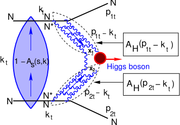
Figure 1: Survival probability for exclusive central diffractive production of the Higgs boson

The structure of the survival probability expression is shown in Fig. 1. The corresponding general formulae for the calculation of the survival probability for diffractive Higgs boson production have been discussed in Refs.SP2CH ; heralhc ; GKLMP . Accordingly,

$$\langle\mid S\mid^{2}\rangle=\frac{N(s)}{D(s)},$$ (IV.17)

$$N(s)=\int d^{2}\,b_{1}\,d^{2}\,b_{2}\{A_{H}(s,b_{1})\,A_{H}(s,b_{2})$$

$$(1-A_{S}(s,(\mathbf{b}_{1}+\mathbf{b}_{2})))\}^{2},$$ (IV.18)

$$D(s)=\int\,d^{2}\,b_{1}\,d^{2}\,b_{2}\{A_{H}(s,b_{1})\,A_{H}(s,b_{2})\}^{2}.$$ (IV.19)

$A_{s}$ denotes the soft strong interaction amplitude given by Eq. (II.5). Using Eq. (II.7)-Eq. (II.9), the integrands of Eq. (IV.18) and Eq. (IV.19) are reduced by eliminating common $s$-dependent expressions.

$$N(s)=\int\,d^{2}b_{1}d^{2}b_{2}\{(1-a_{el}(s,b))A^{pp}_{H}(b_{1})A^{pp}_{H}(b_{2})$$

$$-a_{sd}(s,b)\left(A^{pd}_{H}(b_{1})A^{pp}_{H}(b_{2})+A^{pp}_{H}(b_{1})A^{pd}_{H}(b_{2})\right)$$

$$-a_{dd}(s,b)A^{pd}_{H}(b_{1})A^{pd}_{H}(b_{2})\}^{2},$$ (IV.20)

$$D=\int d^{2}b_{1}d^{2}b_{2}\{A^{pp}_{H}(b_{1})A^{pp}_{H}(b_{2})\}^{2}.$$ (IV.21)

Following Refs.heralhc ; GLM07 we introduce two hard $b$-profiles

$$A^{pp}_{H}(b) = \frac{V_{p\to p}}{2\pi B_{el}^{H}}\exp\left(-\frac{b^{2}}{2\,B_{el}^{H}}\right),$$ (IV.22)

$$A^{pd}_{H}(b) = \frac{V_{p\to d}}{2\pi B_{in}^{H}}\exp\left(-\frac{b^{2}}{2B_{in}^{H}}\right).$$ (IV.23)

The hard radii ${R_{i,k}^{H}}^{2}$ and cross section coefficients $V_{p\to p}$ and $V_{p\to d}$ are constants derived from HERA $J/\Psi$ elastic and inelastic photo and DIS productionKOTE ; PSISL (see, also, Ref.GKLMP ). $B_{el}^{H}=3.6GeV^{-2}$, $B_{in}^{H}=1GeV^{-2}$, $V_{p\to p}=\sqrt{3}$ and $V_{p\to d}=1$. have been taken from the experimental HERA data on $J/\Psi$ production in HERAKOTE ; PSISL .

Using Eq. (IV.17)-Eq. (IV.21) we calculate the survival probability $S^{2}_{H}$ for exclusive Higgs production in central diffraction. $S^{2}_{H}$ has been calculatedheralhc in the two amplitude Model A. The resulting $S^{2}_{H}\,=\,0.027$ is essentially the same as the predictions of KMRKKMR . Our present results, obtained in the three amplitude B Models, indicate a reduction of the output value of $S^{2}_{H}$. Its LHC value in Model B(1) is 0.02, and in Model B(2) it is 0.007. We note that, our Model B(1) result is compatible with the result of Ref.KKMR . We shall return to this issue in the Discussion Section.

V Amplitude Analysis

The basic amplitudes of the GLM two channel model are $A_{1,1}$, $A_{1,2}$ and $A_{2,2}$, whose $b$ structure is specified in Eq. (II.5)). These are the building blocks with which we construct $a_{el}$, $a_{sd}$ and $a_{dd}$ (Eq. (II.7)-Eq. (II.9)). The $A_{i,k}$ amplitudes are bounded by the black disc unitarity bound of unity. Checking Table 1, it is evident that in both Model B(1) and B(2) $\Omega_{2,2}$ is much larger than the other two fitted opacities. As a consequence, the amplitude $A_{2,2}(s,b)$ reaches the unitarity bound of unity at low energies. Similarly, the output amplitude $A_{1,2}(s,b)$ of Model A reaches unity at approximately LHC energy. The observation that one, or even two, of our $A_{i,k}(s,b)$=1 does not imply that the elastic scattering amplitude has reached the unitarity bound at these $(s,b)$ values. $a_{el}(s,b)$ reaches the black disc bound when, and only when, $A_{1,1}(s,b)$=$A_{1,2}(s,b)$=$A_{2,2}(s,b)$=1. In such a case we also obtain, that $a_{sd}(s,b)$=$a_{dd}(s,b)$=0. This result is independent of the fitted value of $\beta$.

Model B(2) predictions of $a_{el}$ over a wide range of energies are presented in Fig. 2. A fundamental feature of Models A, B(1) and B(2) is that $a_{el}$ approaches the black disc bound at $b=0$ very slowly, reaching the bound at energies higher than the GZK knee cutoff. If correct, this feature implies that $a_{el}$ does not reach the black disc bound over the entire accessible spectrum of Cosmic Rays energies, even though it gets monotonically darker.

The explanation of this behavior, in our presentation, is simple. Checking the values of $\beta$ and $\sigma_{i,k}^{0}$ corresponding to the 3 models (see Table 1), we note that $\Omega_{1,1}$ is smaller by 1-3 orders of magnitude relative to $\Omega_{2,2}$ ($\Omega_{1,2}$ in Model A). The consequent $a_{el}$ can reach the black disc bound only when $\Omega_{1,1}$ is large enough so that $A_{1,1}$ approaches unity. $\Omega_{1,1}$ grows slowly like $W^{0.3}$ (modulu $lnW$). Hence, the slow approach of $a_{el}$ toward the black disc bound. This result is incompatible with the output of Ref.KKMR in which $a_{el}$ reaches the black disc bound approximately at the LHC. In our presentation it implies that unlike our models, in the KMR model there is relatively small variance in the weights of the 3 components of the proton wave function.

Figure 2: b dependence of $a_{el}$ in Model B(2) at different energies

A consequence of the input $\Omega_{i,k}$ being large at small $b$, is that $P_{i,k}^{S}(s,b)$ is very small at $b$ = 0 and monotonically approaches its limiting value of 1, in the high $b$ limit. As a result, given a diffractive (non screened) input, its output (screened) amplitude is peripheral in $b$. This is a general feature, common to all eikonal models regardless of their b-profiles details. The same is, true, also, with regard to diffractive Good-Walker channels, which are contained in $\Omega_{i,k}$. This implies a non trivial $t$ dependence of $d\sigma_{diff}(M^{2}_{diff})/dt$ in the diffractive channels. These qualitative features are induced by Model A, B(1) and B(2), even though their detailed behavior are not identical. Given the deficiencies of our b-profiles, we refrain from giving any specific predictions beside the general observation stated above.

The general behavior indicated above becomes more extreme at ultra high energies, when $a_{el}$ continues to expand and gets darker. Consequently, the inelastic diffractive channels becomes more and more peripheral and relatively smaller when compared with the elastic channel. At the extreme, when $a_{el}(s,b)$ = 1, $a_{sd}\,=\,a_{dd}\,=\,0$. We demonstrate this feature and its consequence at the Planck mass in Fig. 2. As the black core of $a_{el}$ expands, the difference between Models A, B(1) and B(2), considered in this paper, diminishes, being confined to the narrow $b$ tail where $a_{el}(s,b)<1$. The above observations may be of interest in the analysis of Cosmic Ray experiments.

VI Discussion

It is interesting to compare our model and its output with a different eikonal model recently proposed by KMRKMR extending earlier versionsKKMR . The two models were constructed with very similar objectives but are fundamentally different in their conceptual theoretical input, data analysis and output results.
1) The input of KMR is a conventional Regge model in which high mass diffraction, initiated by Pomeron enhanced diagrams, is included. GLM is a phenomenological parametrization in which we assume diffraction to be strictly Good-Walker type, with no high mass diffraction distinction. We formulate our input in a general form consistent with Regge, but not exclusively so. Our statistically preferred non factorizeable Model B(2) is compatible with a partonic interpretation which considers the soft ”Pomeron” to be a low $Q^{2}$ high density limit of the hard PomeronSAT . The GLM ”Pomeron” is not a Regge simple J-pole, it does not include Pomeron enhanced diagrams, which are essential in the construction of KMR.
2) Since multi-Pomeron vertices are included in KMR, they had to fix $\alpha^{\prime}=0$. In order to maintain the experimentally observed forward $t$-cone shrinkage, they constructed a high absorption eikonal model in which the input is non conventional $\Delta=0.55$. With this input, KMR obtain an approximate DL behaviorDL in the ISR-Tevatron range. However, at higher energies their effective $\Delta$ becomes monotonically smaller (its value in the Tevatron-LHC range is reduced to 0.04) which results in a very slow rise of $\sigma_{tot}$ and $\sigma_{el}$. GLM is a weak screening eikonal model. Its fitted input is $\Delta=0.15$ and $C=\alpha^{\prime}=0.17$. With this input, GLM total cross sections are compatible with DL over the wide ISR-GZK range.
3) The goal of both GLM and KMR is to adjust the model parameters of their vacuum t exchange ”Pomeron” input, so as to predict and calculate observables and factors of interest at the LHC and Cosmic Rays. Both models adjust more than 10 free parameters. Only CERN-UA4 and Tevatron energies are sufficiently high to justify neglecting the contribution of the secondary Regge sector. This limited data base is not sufficient to adjust the ”Pomeron” free parameters. GLM chose, therefore, to construct a model containing also the secondary Regge sector and fit the extended data base spanning the ISR-Tevatron energy range. KMR constrain their parameter adjustment to the small data base of the highest energies. In our opinion the KMR procedure is not adequate. Indeed, their reconstruction of $\frac{d\sigma_{el}}{dt}$ at the 3 highest available energies is remarkably similar to a fit they made a few years ago with different parameters, notably a conventional $\Delta$ input.
4) GLM and KMR determine their input opacities in completely different procedures which define their (different) data bases. GLM approach is that a model which takes into account diffractive re-scatterings of the initial projectiles has to reconstruct properly the diffractive cross sections, which are, thus, included in its fitted data base. KMR goal is to reconstruct $a_{el}(s,b)$ for which the diffractive components are needed. To this end they fit $\frac{d\sigma_{el}}{dt}$ neglecting an explicit fit of the diffractive channels. Obviously, combining both GLM and KMR data bases is advisable. Regretfully, we were unable to obtain good simultaneous reproduction of such an extended data base. The question, is thus, which model provides a better approximation for the input opacities.
5) The b-distributions of $a_{el}(s,b)$ in GLM are significantly different from KMR. GLM obtain a relatively wide b distribution compared with a narrower one in KMR. $a_{el}(s,b=0)$ in KMR is consistently larger than in GLM, approaching the black disc bound much faster than in GLM. Regardless of these differences, the corresponding values of $\sigma_{tot}$ and $\sigma_{el}$ in both models in the UA4-Tevatron range are compatible. Such compatibility can exist only over a relatively narrow energy band and it cannot persist over a wide energy range. Indeed, the two models have different LHC and Cosmic Rays predictions, which hopefully will be tested soon. Our inability to reproduce $\frac{d\sigma_{el}}{dt}$ outside the narrow forward $t$ cone implies a deficiency in our $a_{el}$ at large $b$. We are not clear if this deficiency is reponsible for the small $S_{H}^{2}$ obtained in our Model B(2). Note, that even though our factorizable Model B(1) has the same feature of spurious dips outside the very forward at $t$ cone, its predicted $S_{H}^{2}$ is 0.02 which is compatible with KMR.
6) In our opinion, the data adjustment procedure adopted by KMR are not adequate. Our approach is to quantify our fit by minimizing its $\chi^{2}$. KMR reject any statistical approach to their data analysis. They tune many of their parameters by eye and refrain from a quantified assessment of their output. The difference between the procedures adopted by the two groups is cardinal, as one is unable to make a systemic evaluation of the KMR output.
7) The difference between the $S_{H}^{2}$ predictions of GLM and KMR are intriguing and reflect the sensitivity of $S_{H}^{2}$ to each model input. $S_{H}^{2}$ is calculated as a convolution of the hard amplitude for Higgs production and the soft probability $P^{S}_{i,k}(s,b)$. The hard amplitude features needed for this calculation in our model are the hard slopes $B^{H}_{el}$, $B^{H}_{in}$ and cross section coefficients $V^{2}_{p\to p}$ $V^{2}_{p\to d}$, determined from the HERA measuredKOTE ; PSISL in $J/\Psi$ photo and DIS elastic and inelastic production. Our sensitivity to these parameters is shown in Fig. 3. Note that when we change the value of $B_{in}^{H}$, we keep the ratio $V^{2}_{p\to d}/B^{H}_{in}$ unchanged. Doing so we do not change the cross section of the reaction $\gamma+p\to J/\Psi+X\mbox{(M $\leq$ 1.6 GeV)}$. KMR calculation is simpler in as much as they consider just the elastic hard slope. In our opinion there is a gap between the sophistication of KMR soft model and the simplicity of their hard approximation. Since $S_{H}^{2}$ is obtained from a convolution of the two terms it is not clear what is the contribution of KMR hard term to the margin of error in their calculation of $S_{H}^{2}$.

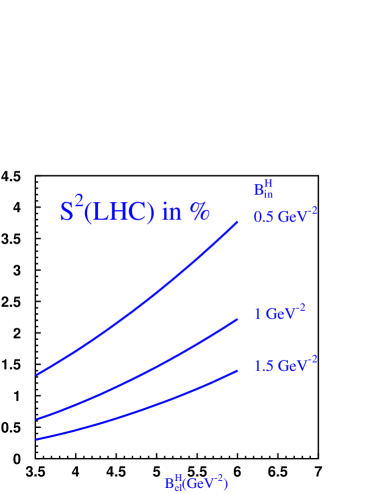
Figure 3: The dependence of $S^{2}$ at the LHC on $B^{H}_{el}$ and $B^{H}_{in}$, the slopes for the hard cross sections.

KMR estimate their margin of uncertainty to be a factor of 2.5. Since our uncertainty derives from similar, though not identical, sources, our assessment is similar. As we saw, both GLM and KMR models are partially deficient. We noted that these are based on the different conceptual constructions and data analysis procedures of the two models. A discrimination between the two models depends on experimental results which are expected to become available within the next few years. In the following we list a few:
1) GLM predictions for $\sigma_{tot}$ and $\sigma_{el}$ at the LHC are 20$\%$ higher than the corresponding KMR values. This is a fundamental difference since the output energy dependence of GLM, which is a weak screening model, is compatible with an effective $\Delta=0.08$ all through the Tevatron-GZK energy range. In the KMR model the effective $\Delta$ is reduced rapidly due to the very strong screening which is inherent to this model. Hence, the KMR cross sections grow very moderately above the Tevatron energy.
2) The difference between the two models becomes more distinguished at Cosmic Rays energies. This may be checked by the Auger experiments where we expect soon some cross section results at energies spanning up to W = 100-150 $TeV$.
3) A basic feature particular to the KMR model is a contribution to diffraction which originates from the Pomeron induced diagrams which are not contained in GLM. As a result, both $\sigma_{sd}$ and $\sigma_{dd}$ predicted by KMR are larger than GLM. These differences are very significant for the DD channel where the KMR prediction at LHC is almost a factor of 3 larger than GLM. Note, that since diffraction in GLM is Good-Walker type, our predicted elastic and diffractive cross sections satisfy the Pumplin boundPumplin , $\sigma_{el}(s,b)+\sigma_{diff}(s,b)\leq\frac{1}{2}\sigma_{tot}$. This bound does not aply to KMR, in which a significant part of its diffractive cross section originate from Pomeron enhanced contributions.
4) An estimate of $S^{2}_{H}$ value can be obtained, at an early stage of LHC operation, through a measurement of the rate of central hard LRG di-jets production (a GJJG configuration) coupled to a study of its expected rate in a non screened pQCD calculation.

Acknowledgments: This research was supported in part by the Israel Science Foundation, founded by the Israeli Academy of Science and Humanities, by BSF grant $\#$ 20004019 and by a grant from Israel Ministry of Science, Culture and Sport and the Foundation for Basic Research of the Russian Federation.

References

- (1) E. Gotsman, E. Levin, U. Maor, E. Naftali and A. Prygarin, ”HERA and the LHC Proceedings Part A” (2005) 221. (arXiv:hep-ph/0511060[hep-ph]).
-
(2)
E. Gotsman, E. Levin and U. Maor,
arXiv:0708.1506v2[hep-ph]. - (3) E. Gotsman, E. Levin and U. Maor, Phys. Rev. D49, (1994) R4321.
- (4) E. Gotsman, E. Levin and U. Maor, Phys. Lett. B452, (1999) 387.
- (5) E. Gotsman, E. Levin and U. Maor, Phys. Rev. D60 (1999) 094011.
- (6) E. Gotsman, H. Kowalski, E. Levin, U. Maor and A. Prygarin, Eur. Phys. J. C47, (2006) 655.
- (7) E. Gotsman, A. Kormilitzin, E. Levin and U. Maor, Eur. Phys. J. C52, (2007) 295.
- (8) J. D. Bjorken, Int. J. Mod. Phys. A7, (1992) 4189; Phys. Rev. D47, (1993) 101.
- (9) E. Gotsman, E.M. Levin and U. Maor, Phys. Lett. B309, (1993) 199.
- (10) T. Affolderr et al., Phys. Rev. Lett. 87, (2001) 141802.
- (11) J. Bartels, E. Gotsman, E. Levin, M. Lublinsky and U. Maor, Phys. Rev. D68 (2003) 054008; Phys.Lett. B556 (2003) 114.
- (12) H.Kowalski and D. Teaney, Phys. Rev. D68 (2003) 114005.
- (13) ZEUS Collaboration, Nucl. Phys. B695 (2004) 3; Eur. Phys. J. C24 (2002) 345.
- (14) V. A. Khoze, A. D. Martin and M. G. Ryskin, Eur. Phys. J. C54 (2008) 199.
- (15) V. A. Khoze, A. D. Martin and M. G. Ryskin, Eur. Phys. J. C18 (2000) 167; Phys. Lett. B643 (2006) 93.
- (16) A. Donnachie and P.V. Landshoff, Nucl. Phys. B231, (1984) 189; Phys. Lett. B296, (1992) 227.
- (17) J.D. Pumplin, Phys. Rev. D8 (1973) 2849.