Abstract: In this communication we introduce a new model which represents the interaction between an atom and two fields injected simultaneously within a cavity including the nonlinear couplers. By using the canonical transformation the model can be regarded as a generalization of several well known models. We calculate and discuss entanglement between the tripartite system of one atom and the two cavity modes. For a short interaction time, similarities between the behavior based on our solution compared with the other simulation based on a numerical linear algebra solution of the original Hamiltonian with truncated Fock bases for each mode, is shown. For a specific value of the Kerr-like medium defined in this paper, we find that the entanglement, as measured by concurrence, may terminate abruptly in a finite time.

PACS: 32.80.-t; 42.50.Ct; 03.65.Ud; 03.65.Yz.

1 Introduction

Recently, the experimental generation of atom–field entangled states in the mesoscopic field regime has been reported for fields with an average photon number of a few tens [1]. Several entanglement measures have been studied, for example the von Neumann reduced entropy [2], the relative entropy of entanglement [3]. Several authors proposed physically motivated postulates to characterize entanglement measures [2]-[5]. Although these postulates vary from one author to another in the details, however they have in common that they are based on the concepts of the operational formulation of quantum mechanics [6]. The entanglement properties have been reported in many different cases [7, 8].

On the other hand, various generalizations of the atom-field interaction models have been considered. One such generalization is to inject two fields simultaneously within a high-$Q$ two-mode bichromatic cavity. In this case the atom interacts with each field individually as well as both fields [9]. In the direction of nonlinear generalization of the atom-field interaction the influence of nonlinear coupling of a cavity mode with a Kerr-like medium on the decay of the excited state of the atom was reported [10, 11]. The nonlinearity can make the dynamics more intricate, for example with respect to switching, modulation and frequency selection of radiation in optical communication networks [12, 13, 14]. In addition, the presence of a nonlinear medium is of particular interest as atom-field dynamics is significantly affected.

This encouraged and stimulated us to investigate a new version of the atom-field interaction model by including the nonlinear couplers. The main goal of this work is to investigate the effect of the nonlinear medium on the phenomenon of entanglement when two fields simultaneously injected within a high-$Q$ cavity. We introduce a way to study tripartite entanglement which is an important issue, by combining two fields and an atom in a double cavity geometry with a Kerr nonlinearity. We also discuss how the nonlinear effects increase in importance compared with increasing atom-field coupling. We show that nonlinear considerations can play a major role in determining the maximum entangled states of the system and generating C-Note gate. Particularly, we employ linear entropy and concurrence to quantify coherence and entanglement, respectively. Beyond fundamental investigations, these results may be of benefit in the characterization of atom-field parameters, and controlling these features may allow for new control techniques for single and multiple qubit coupling.

The paper is organized as follows: In section 2 we describe the model and the analytical approach which based on the canonical transformation. In Sec. 3 we briefly comment on the collapse-revival phenomena. In Sec. 4 we identify the different regimes of entanglement due to the linear entropy and concurrence. Sec. 5 presents some concluding remarks.

2 The model and its solution

We devote this section to introduce our model taking into consideration the effect of a Kerr-like medium (nonlinear couplers). For this reason let us make our starting point the Hamiltonian

$$\hat{H}=\hat{H}_{\mathrm{f}}+\hat{H}_{\mathrm{a}}+\hat{H}_{\mathrm{af}},$$ (1)

where $\hat{H}_{\mathrm{f}}$ comprises a field-field interaction (parametric down conversion model) in the presence of a nonlinear Kerr medium given by

$$\hat{H}_{\mathrm{f}}=\sum_{i=1}^{2}\hslash\left[\left(\omega_{i}\hat{a}_{i}^{\dagger}\hat{a}_{i}+\chi_{i}\hat{a}_{i}^{\dagger 2}\hat{a}_{i}^{2}\right)+\bar{\chi}\hat{a}_{1}^{\dagger}\hat{a}_{1}\hat{a}_{2}^{\dagger}\hat{a}_{2}\right]+\hslash\lambda\left(\hat{a}_{1}^{\dagger}\hat{a}_{2}+\hat{a}_{2}^{\dagger}\hat{a}_{1}\right),$$ (2)

where $\chi_{i},i=1,2$ and $\bar{\chi}$ are related to the cubic susceptibility of the medium, such that $\chi_{i},i=1,2$  represent the self-action for each mode, while $\bar{\chi}$ is related to the cross-action processes, respectively [16]. The other two parts of the Hamiltonian consists of the atom-field interaction and the free atomic system that is

$$\hat{H}_{\mathrm{a}}=\frac{\omega_{0}}{2}\hslash\hat{\sigma}_{z},\mathrm{\ \ \ \ \ \ \ }\hat{H}_{\mathrm{af}}=\sum_{i=1}^{2}\hslash\lambda_{i}\left(\hat{a}_{i}\hat{\sigma}_{+}+\hat{a}_{i}^{\dagger}\hat{\sigma}_{-}\right).$$ (3)

The Hamiltonian (2) can be regarded as a generalization of models considered earlier in the absence of the Kerr-like medium, see for example [17], which concentrate on studying entropy squeezing as well the degree of entanglement. In order to consider the statistical properties of the present system we have to find the dynamical operators either by solving the equations of motion in the Heisenberg picture, or by finding the wave function in the Schrödinger picture.

The latter case will be adopted. To reach our goal let us first introduce the canonical transformation

$$\left(\begin{array}[]{c}\hat{a}_{1}\\ \hat{a}_{2}\end{array}\right)=\left(\begin{array}[]{cc}\cos\theta&\sin\theta\\ -\sin\theta&\cos\theta\end{array}\right)\left(\begin{array}[]{c}\hat{b}_{1}\\ \hat{b}_{2}\end{array}\right),$$ (4)

with the properties

$$\hat{a}_{1}^{\dagger}\hat{a}_{1}+\hat{a}_{2}^{\dagger}\hat{a}_{2}=\hat{b}_{1}^{\dagger}\hat{b}_{1}+\hat{b}_{2}^{\dagger}\hat{b}_{2},$$ (5)

where $[\hat{a}_{i},\hat{a}_{j}^{\dagger}]=[\hat{b}_{i},\hat{b}_{j}^{\dagger}]=\delta_{ij}.$ Since the total energy for the system before the rotation is equal to that after rotation and hence the transformation is invariant. Thus, with a particular choice of the angle $\theta,$ the above transformation would enable us to remove the evanescent waves term from the Hamiltonian (2). This can be achieved if we take

$$\theta=\frac{1}{2}\tan^{-1}\left(\frac{2\lambda}{\omega_{2}-\omega_{1}}\right).$$ (6)

In this case the Hamiltonian (2) reduces to

$$\hat{H}=\sum_{i=1}^{2}\hslash\left[\left(\Omega_{i}\hat{b}_{i}^{\dagger}\hat{b}_{i}+\chi\hat{b}_{i}^{\dagger 2}\hat{b}_{i}^{2}\right)+\mu_{i}\left(\hat{b}_{i}\hat{\sigma}_{+}+\hat{b}_{i}^{\dagger}\hat{\sigma}_{-}\right)\right]+\hslash\chi\sum_{i\neq j=1}^{2}\hat{b}_{i}^{\dagger}\hat{b}_{i}\hat{b}_{j}^{\dagger}\hat{b}_{j}+\frac{\omega_{0}}{2}\hslash\hat{\sigma}_{z},$$ (7)

where we have assumed the cross-action coupling parameter is equal to twice the self-action parameter of each mode, so that $\chi_{1}=\chi_{2}=\chi=\frac{1}{2}\bar{\chi}$ (codirectional coupler case). Further, we have also defined

$$\Omega_{1}=\left(\omega_{1}\cos^{2}\theta+\omega_{2}\sin^{2}\theta-\lambda\sin 2\theta\right)^{\frac{1}{2}},\qquad\Omega_{2}=\left(\omega_{2}\cos^{2}\theta+\omega_{1}\sin^{2}\theta+\lambda\sin 2\theta\right)^{\frac{1}{2}},$$ (8)

and

$$\mu_{1}=\lambda_{1}\cos\theta-\lambda_{2}\sin\theta,\qquad\mu_{2}=\lambda_{2}\cos\theta+\lambda_{1}\sin\theta.$$ (9)

Finally, let us adjust the coupling parameter $\lambda$ to take the form

$$\lambda=\lambda_{1}\lambda_{2}\left(\frac{\omega_{2}-\omega_{1}}{\lambda_{2}^{2}-\lambda_{1}^{2}}\right),$$ (10)

from which the interaction Hamiltonian $V^{I}(t)$ can be written thus

$$V^{I}(t)=\bar{\mu}\left(\hat{b}_{2}\hat{\sigma}_{+}\otimes\exp\left(-i[\Delta+2\chi(\hat{b}_{1}^{\dagger}\hat{b}_{1}+\hat{b}_{2}^{\dagger}\hat{b}_{2}-1]t\right)+c.c\right),$$ (11)

where $\bar{\mu}=\sqrt{\lambda_{1}^{2}+\lambda_{2}^{2}}$ and $\Delta=\Omega_{2}-\omega_{0}.$ Having obtained the interaction picture, we are therefore in a position to find the explicit solution of the wave function and consequently the density matrix. After some calculations the density matrix of the system can be written as

$$\hat{\rho}(t)=U(t)\hat{\rho}(0)U^{\dagger}(t),$$ (12)

where $U(t)$ is a $2\times 2$ matrix representing the time evolution operator; its elements are

$$U_{11}(t) = \left[\cos\delta_{m_{1},m_{2}}^{+}t+i\frac{\Gamma_{m_{1},m_{2}}}{2\delta_{m_{1},m_{2}}^{+}}\sin\delta_{m_{1},m_{2}}^{+}t\right]\exp(-i\Gamma_{m_{1},m_{2}}t),$$

$$U_{12}(t) = (U_{12})^{\ast}=-i\bar{\mu}\sqrt{m_{2}+1}\frac{\sin\delta_{m_{1},m_{2}}^{+}t}{\delta_{m_{1},m_{2}}^{+}}\exp(-i\Gamma_{m_{1},m_{2}}t),$$

$$U_{22}(t) = \left[\cos\delta_{m_{1},m_{2}}^{-}t-i\frac{\Gamma_{m_{1},m_{2}}}{2\delta_{m_{1},m_{2}}^{-}}\sin\delta_{m_{1},m_{2}}^{-}t\right]\exp(i\Gamma_{m_{1},m_{2}}^{\prime}t),$$ (13)

$$\ \delta_{m_{1},m_{2}}^{+} = \left[\frac{1}{4}\Gamma_{m_{1},m_{2}}^{2}+\bar{\mu}^{2}(m_{2}+1)\right]^{\frac{1}{2}},\qquad\delta_{m_{1},m_{2}}^{-}=\left[\frac{1}{4}\Gamma_{m_{1},m_{2}}^{2}+\bar{\mu}^{2}m_{2}\right]^{\frac{1}{2}},$$

$$\Gamma_{m_{1},m_{2}} = \Delta+2\chi(m_{1}+m_{2}-1),\qquad\Gamma_{m_{1},m_{2}}^{\prime}=\Delta+2\chi(m_{1}+m_{2}-2).$$ (14)

3 Atomic inversion

For applications in real systems, one can see the atomic inversion of the two-level system is of particular interest. Therefore, in the present communication we discuss the time dependence of the two-level-system observable $\langle\hat{\sigma}_{z}(t)\rangle$, for different values of the Kerr-like medium. The usual coherent state is used as initial conditions for the fields. As might be expected, the behavior of the two-level system changes dramatically depending on the value of the non-linear medium.

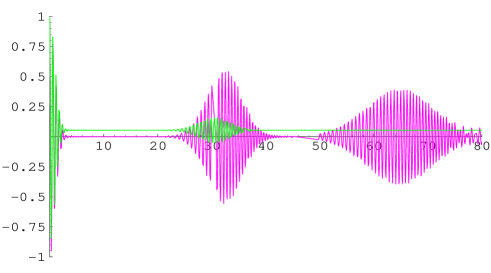
Figure 1: Atomic inversion as a function of the scaled time $\lambda_{1}t$. The parameters are $\lambda_{2}/\lambda_{1}=0.01,\omega_{1}/\lambda_{1}=0.2,\omega_{2}/\lambda_{1}=0.1,\Delta/\lambda_{1}=0,\chi/\lambda_{1}=0$, and $\bar{n}_{1}=\bar{n}_{2}=10$. The initial state is $|\alpha_{1},\alpha_{2};e\rangle$, where $\alpha_{i}=|\alpha_{i}|e^{i\phi},$ $\chi/\lambda_{1}=0.001$ (solid curve) and $\chi/\lambda_{1}=0.1$ for (dots).

In Fig. (1) we have plotted the atomic inversion as a function of the scaled time $\lambda_{1}t$ for different values of the Kerr-like medium and the phase of coherent states is taken to be zero i.e. $\phi=0$. It has been observed that for a small value of the Kerr-like medium such as $\chi/\lambda_{1}=0.001,$ the system shows period of collapse after onset of the interaction. This is followed with a long period of the revival. Here we may point out that comparing with the first period of collapse the amplitude of the oscillations for the second period is decreased, see fig.(1) (solid curve). This means that as the time of the interaction increases the amplitude of the oscillations decreases. Increasing the value of the Kerr-like medium leads to increase in the period of collapses with decreasing in the size of the amplitude of each period, see fig.(1) (dot curve). It is also noted that as a special case of the model when $\lambda_{2}=\chi_{2}=0$, the general behavior of the atomic inversion coincides with that of the well known JCM in presence of the Kerr-like medium [18].

We have verified the behavior obtained in the numerical simulations based on the final equations and the numerical solutions of the original Hamiltonian i.e. one simulation simply based on the final equations and the other simulation based on a numerical linear algebra solution of the original Hamiltonian with truncated Fock bases for each mode (see Fig. 2). Provided the ratio $\lambda_{2}/\lambda_{1}$ is made small enough, we have excellent agreement for the short time scales. In the meantime, the value $\lambda_{2}/\lambda_{1}=0.01$ gives quantitative agreement over some periods of oscillation.

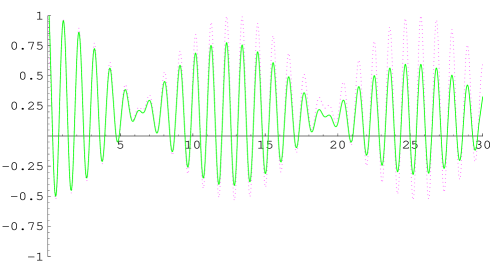
Figure 2: Atomic inversion as a function of the scaled time $\lambda_{1}t$. The parameters are $\lambda_{2}/\lambda_{1}=0.01,\omega_{1}/\lambda_{1}=0.2,$ $\chi/\lambda_{1}=0.01$ $\omega_{2}/\lambda_{1}=0.1,$ $\Delta/\lambda_{1}=0,$ $\chi/\lambda_{1}=0.01$. The initial state is $|5,6;e\rangle$, where dotted curve obtained using the final equations and solid curve obtained using linear algebra solution of the original Hamiltonian.

The revival time for the present system is calculated to give us

$$t_{R}=\frac{2n\pi}{\lambda\left(\Omega_{\bar{n}}-\Omega_{\bar{n}-1}\right)},$$ (15)

where $\Omega_{\bar{n}}$ is the Rabi frequency, such that $\Omega_{\bar{n}}=\delta_{\overline{m}_{1},\overline{m}_{2}}^{+}\$and $n$ is an integer,

$$\lambda_{1}t_{R} = \frac{2n\pi}{\lambda\Delta\chi^{\prime}+\chi^{\prime 2}(4\bar{n}-3)-\overline{\mu}^{\prime 2}}\left\{\frac{1}{2}\sqrt{(2\chi^{\prime}(2\bar{n}-1)+\Delta^{\prime})^{2}+\overline{\mu}^{\prime 2}(\bar{n}+1)}\right.$$ (16)

$$+\left.\frac{1}{2}\sqrt{(2\chi^{\prime}(2\bar{n}-2)+\Delta^{\prime})^{2}+\overline{\mu}^{\prime 2}\bar{n}}\right\},$$

where $\chi^{\prime}=\chi/\lambda_{1},$ $\overline{\mu}^{\prime}=\overline{\mu}^{\prime}/\lambda_{1},$ $\Delta^{\prime}=\Delta/\lambda_{1}.$ In the following section we turn our attention to discuss the effect of the Kerr-like medium on the phenomenon of entanglement.

4 Entanglement

In this section we shall concentrate on the discussion of the entanglement where the total state vector can not be written precisely as the product of a time-dependent atomic and field component vector.

4.1 Coherence loss

Distillable entanglement is a critical resource for quantum information. In our case we are considering transduction of quantum information between fields and atoms so the degree of entanglement between the atom and the field is important to assess its use in quantum information. Furthermore there are three entities: two field modes and one atom, and the entanglement between any single entity and the other two can be used so we assess the inherent resource in our system by calculating the tripartite entanglement in the combined system.

Here we use the idempotency defect [19], defined by linear entropy, as a measure of the degree of mixture for a state $\hat{\rho}_{a}(t).$ This version of entropy makes the problem tractable [20] and therefore we use this idempotency defect as a measure of coherence loss. This is given by

$$\mathcal{E}_{t}^{(a)}=\mathrm{Tr}\big{[}\hat{\rho}_{a}(t)\left(1-\hat{\rho}_{a}(t)\right)\big{]},$$ (17)

where $\mathcal{E}_{t}^{(a)}$ has a zero value for a pure state and $1$ for a completely mixed state.

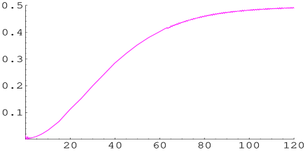
Figure 3: Linear entropy as a function of the scaled time $\lambda_{1}t$. The parameters are $\lambda_{2}/\lambda_{1}=0.1,\omega_{1}/\lambda_{1}=0.2,\omega_{2}/\lambda_{1}=0.1,\Delta/\lambda_{1}=0,\chi/\lambda_{1}=0$, and $\bar{n}_{1}=\bar{n}_{2}=10$. The initial state is $\frac{1}{\sqrt{2}}(|e\rangle+|g\rangle)\otimes|\alpha_{1},\alpha_{2}\rangle$, where (a) $\chi/\lambda_{1}=0.001$ and (b) $\chi/\lambda_{1}=0.01$.

In Fig. (3) we have plotted the idempotency defect as a function of the scaled time for different values of the Kerr-like medium. It is shown that the asymptotic value of the linear entropy is obtained when the time is increased. Also the value of $\mathcal{E}_{t}^{(a)}$ increases as the time increases in addition to the appearance of irregular fluctuations at discrete period of time for a large value of the Kerr-like medium, see fig.(3b). Of course, there are some differences between the two cases (small and large values of the Kerr-like medium) in the amplitudes but the general behavior is the same. This may be thought to arise from the asymptotic limits which have been observed in both Figs. 3(a,b).

4.2 Tripartite Quantum States

Now we would like to discuss an example of entanglement between the two cavity fields and atom. In the case of pure state, if the density matrix obtained from the partial trace over other subsystems is not pure the state is entangled. Consequently, for the pure state of a bipartite system, entropy of the density matrix associated with either of the two subsystems is a good measure of entanglement. In the mixed state case, the entanglement can be quantified by the quantity $C(\rho)$ which is known in literature as concurrence. Quite recently, some approaches have been reported for the determination of entanglement in experiment [21, 22, 23, 24]. The most remarkable are the new formulation of concurrence [24] in terms of copies of the state which led to the first direct experimental evaluation of entanglement and some analogous contributions [25] to multipartite concurrence.

For the density matrix $\hat{\rho}(t),$ which represents the state of a bipartite system, concurrence is defined as [26]

$$C(\hat{\rho})=\max\{0,\mathit{\lambda}_{1}-\mathit{\lambda}_{2}-\mathit{\lambda}_{3}-\mathit{\lambda}_{4}\},$$ (18)

where the $\mathit{\lambda}_{i}$ are the non-negative eigenvalues, in decreasing order ($\mathit{\lambda}_{1}\geq\mathit{\lambda}_{2}\geq\mathit{\lambda}_{3}\geq\mathit{\lambda}_{4}$), of the Hermitian matrix

$$\widehat{\Upsilon}\equiv\sqrt{\sqrt{\hat{\rho}}\widetilde{\rho}\sqrt{\hat{\rho}}},\,\widetilde{\rho}=\left(\widehat{\sigma}_{y}\otimes\widehat{\sigma}_{y}\right)\hat{\rho}^{\ast}\left(\widehat{\sigma}_{y}\otimes\widehat{\sigma}_{y}\right).$$ (19)

Here, $\hat{\rho}^{\ast}$ represents the complex conjugate of the density matrix $\hat{\rho}$ when it is expressed in a fixed basis and $\widehat{\sigma}_{y}$ represents the Pauli matrix in the same basis. The function $C(\hat{\rho})$ ranges from $0$ for a separable state to $1$ for a maximum entanglement.

We first investigate the quantum correlation between the atom and cavity modes. If we consider the initial state of the system is given by $\rho(0)=\gamma|0,1;e\rangle\langle 0,1;e|+\beta|0,1;g\rangle\langle 0,1;g|,$ $\gamma+\beta=1,$ which means that the atom starts from a mixed state and the field starts from $|0,1\rangle$ state i.e. the vacuum for the first mode and one photon in the other mode. If we deal with the two cavity modes as system $A$, and the atom as system $B$, then $\rho(t)$ in equation (12) can be thought of as the density operator of a two-qubit mixed state. In the basis $|1\rangle\equiv|01\rangle\otimes|e\rangle$, $|2\rangle\equiv|01\rangle\otimes|g\rangle$, $|3\rangle\equiv|00\rangle\otimes|e\rangle$, $|4\rangle\equiv|02\rangle\otimes|g\rangle$, the density matrix can be written as [27]

$$\rho(t)=\left(\begin{array}[]{c}\rho_{11}\\ 0\\ 0\\ \rho_{41}\end{array}\begin{array}[]{c}0\\ \rho_{22}\\ \rho_{32}\\ 0\end{array}\begin{array}[]{c}0\\ \rho_{23}\\ \rho_{33}\\ 0\end{array}\begin{array}[]{c}\rho_{14}\\ 0\\ 0\\ \rho_{44}\end{array}\right).$$ (20)

where $\rho_{ij}=\langle i|\rho(t)|j\rangle.$

The explicit expression of the concurrence describing the entanglement between the system $A$ and system $B$ can be found using equations (18) and (20) as

$$C(\rho)=2\max\left\{0,|\rho_{23}|-\sqrt{\rho_{11}\rho_{44}},|\rho_{14}|-\sqrt{\rho_{22}\rho_{33}}\right\},$$ (21)

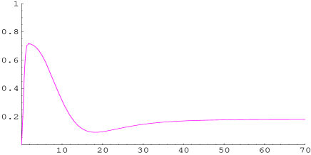
Figure 4: Concurrence as a function of the scaled time $\lambda_{1}t$. The parameters are $\lambda_{2}/\lambda_{1}=0.1,\omega_{1}/\lambda_{1}=0.2,\omega_{2}/\lambda_{1}=0.1,\Delta/\lambda_{1}=0,\chi/\lambda_{1}=0$. The initial state is $\rho(0)=\frac{1}{2}(|e\rangle\langle e|+|g\rangle\langle g|)\otimes|0,1\rangle\langle 0,1|$, where (a) $\chi/\lambda_{1}=0.001$ and (b) $\chi/\lambda_{1}=0.01$.

The graphs of the concurrence as a function of time for the two dynamical regimes are displayed in Fig. 4. Keeping the value of the Kerr-like medium small enough, the asymptotic value of the concurrence is not null, since the global system evolves to a classically correlated state. But once the $\chi/\lambda_{1}$ is increased we see that the concurrence vanishes in the asymptotic limit. With increasing $\chi/\lambda_{1}$ further, we note that the decay of the concurrence is more rapid than the corresponding decay in the weak nonlinear regime.

If the initial state has been considered such as $\gamma=1,$ then the sudden death of entanglement will be obtained if $\rho_{11}\rho_{44}=0.$ This means that the sudden death time is given by

$$\lambda_{1}t_{d}=\frac{1}{2\chi^{\prime}-\Delta^{\prime}}\cos^{-1}\left(\frac{2\left(\Delta^{\prime}-2\chi^{\prime}\right)^{2}}{\left(\Delta^{\prime}-2\chi^{\prime}\right)^{2}-8\left(1+\lambda_{2}^{\prime 2}\right)}\right).$$ (22)

In the limit that the fields decouple from the atom, it is shown that, one may just entangling the cavity fields along the lines which has been considered in Ref. [28].

In quantum computation operations are performed by means of single-qubit and multiple-qubit quantum logic gates. In what follows we consider universal quantum logic gate based on two electromagnetic field modes of a cavity. From equation (12), we can get various time evolutions of the present system. If the initial state is taken to be $|e\rangle,$ and we set

$$\chi=\frac{\lambda_{1}}{2}\sqrt{4-\overline{\mu}^{2}},$$ (23)

then, to obtain the C-NOT gate, we need the unitary operation with $\chi=\frac{\lambda_{1}}{2}\sqrt{4-\overline{\mu}^{2}},$ $\Delta=0,$ and interaction time $\lambda_{1}t=2n\pi$, ($n=1,2,3,...$) which gives

$$|e\rangle_{a}|0,0\rangle_{f} \mapsto |e\rangle_{a}|0,0\rangle_{f}\mapsto|e\rangle_{a}|0,0\rangle_{f}\mapsto|e\rangle_{a}|0,0\rangle_{f},$$

$$|g\rangle_{a}|0,1\rangle_{f} \mapsto |g\rangle_{a}|0,1\rangle_{f}\mapsto|g\rangle_{a}|0,1\rangle_{f}\mapsto|g\rangle_{a}|0,1\rangle_{f},$$ (24)

i.e. using a specific values of the Kerr-like medium in the present model, one can be able to implement a C-NOT gate.

5 Conclusion

In this paper we have discussed a new Hamiltonian class which describes the the interaction between a single two-level atom and bimodal cavity field taking into account an optical Kerr nonlinearity. We present an analytically solution and numerical investigation of the atomic inversion, coherence loss and entanglement. Entanglement of the tripartite system of one atom and the two cavity modes has been discussed and the sudden death of entanglement is shown. Also, we proposed a scheme for quantum computing (C-NOT gate), which is realized by a nonlinear interaction in the QED cavity. For our model to be useful for experiments, we would need to include cavity losses, fluorescence, and atomic motion. These extensions to our model could be accomplished by standard master equation methods, and such an analysis is reserved for future work. Our purpose here has been to develop a Hamiltonian that includes many of the iconic Hamiltonians used in quantum optics as special cases so that three coupled systems are used, which opens up investigations from bipartite to tripartite entanglement. Cavity quantum electrodynamics with one atom and two fields, including a nonlinear interaction, creates rich, interesting dynamics as shown here.

Acknowledgements:

B C Sanders¹, M. S. Abdalla² and M. Abdel-Aty³ are grateful for the financial support from iCORE and a CIFAR Associateship¹, the project Math 2008/132 of the research center, College of Science, King Saud University² and the project No. 11/2008 Bahrain University³.

References

- [1] A. Auffeves, P. Maioli, T. Meunier, S. Gleyzes, G. Nogues, M. Brune, J.M. Raimond, S. Haroche, Phys. Rev. Lett. 91, 230405 (2003).
- [2] J von Neumann, Mathematische Grundlagen der Quantenmechanik, Springer, Berlin, 1932.
- [3] M. B. Plenio, V. Vedral, Phys. Rev. A 57, 1619 (1998).
- [4] M. Horodecki, P. Horodecki, R. Horodecki, Phys. Rev. Lett. 84, 2014 (2000); F. Saif, M. Abdel-Aty, M. Javed, and R. Ul-Islam, Appl. Math. Inf. Sci. 1, 323 (2007).
- [5] M. A. Nielsen, I. L. Chuang, Quantum Computation and Quantum Information (Cambridge University Press, Cambridge, 2000).
- [6] K. Kraus, States, Effects and Operations, Springer, Berlin, 1983.
- [7] J. Gea-Banacloche, T. C. Burt, P. R. Rice, L. A. Orozco, Phys. Rev. Lett. 94, 053603 (2005).
- [8] A. Delgado, A. B. Klimov, J. C. Retamal, C. Saavedra, Phys. Rev. A 58, 655 (1998).
- [9] M. S. Abdalla, A.-S. F. Obada and M. Abdel-Aty, Ann. Phys. 318, 266 (2005).
- [10] B. W. Shore, P. L. Knight, J. Mod. Opt. 40, 1195 (1993).
- [11] S. M. Barnett, P. L. Knight, J. Opt. Soc. Am. B 3, 467 (1985); S. M. Barnett, P. L. Knight, J. Mod. Opt. 43, 841 (1987); P. Gora, C. Jedrzejek, Phys. Rev. A 45, 6816 (1992); V. Buzek, I. Jex, Opt. Commun. 78, 425 (1990); H. Moya-Cessa, V. Buzek, P. L. Knight, Opt. Commun. 85, 287 (1991).
- [12] J. Fiurášek, J. Křepelka and J. Peřina, Opt. Comm. 167, 115 (1999).
- [13] G. Ariunbold and J. Peřina, Opt. Commun. 176, 149 (2000).
- [14] F. A. A. El-Orany, M. S. Abdalla and J Peřina, J. Opt. B: Quant. Semiclass. Opt. 67, 460 (2004).
- [15] P. A. M. Netto, L. Davidovich, and J. M. Raimond, Phys. Rev. A 43, 5073 (1991).
- [16] M. S. Abdalla, J. Křepelka, and J. Peřina, J. Phys. B: At. Mol. Opt. Phys. 39, 1563 (2006).
- [17] M. S. Abdalla, M. Abdel-Aty and A.-S. F. Obada, Opt. Commun. 211, 225 (2002); J. Opt. B: Quant. Semiclass.Opt. 4, 396 (2002); J. Phys. B: At. Mol. Opt. Phys. 35, 4773 (2002).
- [18] V. Buzek, I. Jex, Opt. Commun. 78, 425 (1990); A.-S. F. Obada, M. M. A. Ahmed, F. K. Faramawy, E. M. Khalil, Chaos, Solitons & Fractals, 28, 983 (2006).
- [19] W. H. Zurek, S. Habib, and J. P. Paz, Phys. Rev. Lett. 70, 1187 (1993).
- [20] D. W. Berry and B. C. Sanders, J. Phys. A: Math. Gen. 36 12255 (2003).
- [21] S. P. Walborn, P. H. S. Ribeiro, L. Davidovich, F. Mintert and A. Buchleitner, Phys. Rev. A 75, 032338 (2007).
- [22] S. P. Walborn, P H S Ribeiro, L. Davidovich, F. Mintert and A. Buchleitner, Nature 440, 1022 (2006).
- [23] F. Mintert and A. Buchleitner, Phys. Rev. Lett. 98, 140505 (2007).
- [24] F. Mintert, A. R. R. Carvalho, M. Kuś, A Buchleitner, Phys. Rep. 415, 207 (2005).
- [25] L. Aolita and F. Mintert, Phys. Rev. Lett. 97, 050501 (2006).
- [26] W. K. Wootters, Phys. Rev. A 80, 2245 (1998).
- [27] E. Santos and M Ferrero, Phys. Rev. A 62, 024101 (2000); C. H. Bennett, H. J. Bernstein, S. Popescu, B. Schumacher, Phys. Rev. A 53, 2046 (1996) ; W. J. Munro, D. F. V. James, A. G. White, and P. G. Kwiat, Phys. Rev. A 64, 030302 (2001).
- [28] B. C. Sanders, Phys. Rev. A 45, 6811 (1992); 46, 2966 (1992).