Influence of Compton scattering on the broad-band X-ray spectra of intermediate polars

Abstract

Context. The majority of cataclysmic variables observed in the hard X-ray energy band are intermediate polars where the magnetic field is strong enough to channel the accreting matter to the magnetic poles of the white dwarf. A shock above the stellar surface heats the gas to fairly high temperatures (10–100 keV). The post-shock region cools mostly via optically thin bremsstrahlung.

Aims. We investigate the influence of Compton scattering on the structure and the emergent spectrum of the post-shock region. We also study the effect it has on the mass of the white dwarfs obtained from fitting the observed X-ray spectrum of intermediate polars.

Methods. We construct the model of the post-shock region taking Compton scattering into account. The radiation transfer equation is solved in the plane-parallel approximation. The feedback of Compton scattering on the structure of the post-shock region is also accounted for. A set of the post-shock region model spectra for various white dwarf masses is calculated.

Results. We find that Compton scattering does not change the emergent spectra significantly for low accretion rates or low white dwarf masses. However, it becomes important at high accretion rates and high white dwarf masses. The time-averaged, broad-band X-ray spectrum of intermediate polar V709 Cas obtained by the RXTE  and INTEGRAL observatories is fitted using the set of computed spectral models. We obtained the white dwarf mass of 0.91 $\pm$ 0.02 $M_{\odot}$ and 0.88 $\pm$ 0.02 $M_{\odot}$ using models with Compton scattering taken into account and without it, respectively.

Conclusions.

1 Introduction

Cataclysmic variables (CVs) are close binary systems with a white dwarf (WD) as a primary (Warner, 1995). A WD accretes matter from a companion star (typically a red dwarf) that fills its Roche lobe. This matter forms an accretion disc inside the Roche lobe of the WD. In intermediate polars (IPs), the significant magnetic field (10⁶–10⁷ G) can disrupt the disc at some distance from the WD surface. The matter is then free-falling along the magnetic field lines onto the WD and forms a strong shock above its surface (Aizu, 1973). The temperature in the post-shock region (PSR) can be very high ($\sim$10–100 keV) and the plasma there is cooled mainly via optically thin bremsstrahlung radiation in the X-ray band (Fabian et al., 1976; Lamb & Masters, 1979; King & Lasota, 1979). Cooling via Compton scattering is less significant due to a relatively low radiation energy density in PSR. This contrasts with the accretion columns of X-ray pulsars, where Comptonization is the dominant cooling mechanism (see Becker & Wolff 2007, for more details).

The theory of the PSR has been developed in a number of papers (Aizu, 1973; Wu et al., 1994; Woelk & Beuermann, 1996; Cropper et al., 1999). The most recent investigations by Canalle et al. (2005) and Saxton et al. (2005, 2007) have studied the role of the two-temperature plasma and considered the dipole magnetic funneling (not the standard plane-parallel approximation). The plasma temperature in the PSR depends on the free-fall velocity at the WD surface; therefore, the X-ray spectra of IPs can be used to determine the WD mass (Rothschild et al., 1981). Such studies have been performed by Cropper et al. (1998), Cropper et al. (1999), Ramsay (2000), Beardmore et al. (2000), Revnivtsev et al. (2004), Suleimanov et al. (2005), and Falanga et al. (2005), using various X-ray data sets. Suleimanov et al. (2005) demonstrated that, to accurately measure the maximum post-shock temperature to infer the WD mass, the spectra at high energies (up to at least 100 keV) are needed.

The IPs are the most luminous and the hardest X-ray sources among accreting WDs. The interest in this class of objects has been growing in the past few years as IPs have been recently proposed as the dominant X-ray source population detected near the Galactic centre by Chandra observatory (Muno et al., 2004; Ruiter et al., 2006). The IPs also contribute significantly to the X-ray diffuse Galactic ridge emission (Revnivtsev et al., 2006), as well as dominate the hard X-ray sky there (Krivonos et al., 2007a). Moreover, most of the known CVs detected by INTEGRAL (Bird et al., 2007; Krivonos et al., 2007b) and Swift satellites are IPs (see e.g. Barlow et al., 2006; Bonnet-Bidaud et al., 2007; de Martino et al., 2008). In the strongly magnetized ($B\geq 10^{7}$ G) polar systems, cyclotron radiation is an important cooling mechanism, which suppresses the high temperature bremsstrahlung emission, whilst it should be negligible for the IPs. This could explain why the majority of the CVs observed in the hard X-ray band are IPs.

To better understand the hard X-ray production in IPs, one needs to model their observed spectral properties. The goal of the present paper is to investigate the influence of Compton scattering on the structure of the PSR and the emergent spectrum. We developed the physical model of the PSR and compare the computed spectral models to the broad-band X-ray spectrum of the intermediate polar V709 Cas obtained by RXTE and INTEGRAL observatories. We have also determined the WD mass in this system.

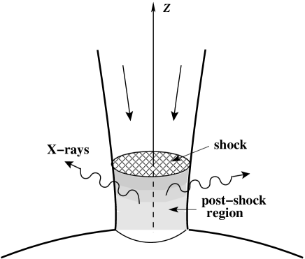
Figure 1: A schematic view of the accretion flow onto the WD magnetic polar cap. The accreting gas falls quasi-radially towards the magnetic poles, forming a standing shock, below which the X-rays are emitted.

2 Model of the post-shock region

2.1 Main equations

The structure of the stationary post-shock region (the accretion and emission geometry is illustrated schematically in Fig. 1) in a plane-parallel, one-dimensional geometry can be described (see e.g. Cropper et al., 1999; Suleimanov et al., 2005) by the mass continuity equation

$$\frac{{\rm d}}{{\rm d}z}(\rho V)=0,$$ (1)

the momentum equation

$$\frac{{\rm d}}{{\rm d}z}(\rho V^{2}+P)=-\frac{GM_{\rm wd}}{(z+R_{\rm wd})^{2}}\rho,$$ (2)

the energy equation

$$V\frac{{\rm d}P}{{\rm d}z}+\gamma P\frac{{\rm d}V}{{\rm d}z}=-(\gamma-1)(1+A)\Lambda,$$ (3)

and the ideal-gas law

$$P=\frac{\rho kT}{\mu m_{\rm H}}.$$ (4)

Here $m_{\rm H}$ is the hydrogen mass and $\gamma$=5/3 is the adiabatic index. The cooling rate $\Lambda$ due to thermal optically thin radiation is given by

$$\Lambda=n_{\rm e}n_{\rm i}\Lambda_{\rm N}(T),$$ (5)

where $\Lambda_{\rm N}(T)$ is the cooling function, $n_{\rm e}$ the electron number density, and $n_{\rm i}$ the ion number density. We take $\Lambda_{\rm N}(T)$ for solar chemical composition as calculated and tabulated by Sutherland & Dopita (1993).

The term $1+A$ is the amplification factor due to Comptonization. In contrast to the usually used integral amplification factor (which is just the ratio of the emergent flux to the incident flux of some seed soft photons, see Illarionov & Sunyaev 1975; Svensson 1984), we use here the local amplification factor, because we are interested in the vertical structure of the accretion column. In a homogeneous isothermal slab, the integral and local factors are nearly equal. As the Compton cooling rate depends on the local plasma temperature and density in a different way compared to the optically thin, thermal radiation, the local amplification factor $(1+A)$ is a function of the geometrical coordinate $z$. The cooling due to cyclotron radiation is not considered here.

Equation (1) has the integral

$$\rho V=a,$$ (6)

where the mass accretion rate $a$ per unit area is a free parameter of the model.

A simple analytical solution of Eqs. (1)–(4) can be obtained (see Frank et al., 2002), if one assumes a constant gas pressure throughout the PSR and considers the cooling only by bremsstrahlung. The distributions of the velocity, temperature, and density along the PSR height $z$ in this case are

$$V=V_{0}\left(\frac{z}{H_{\rm s}}\right)^{2/5},\leavevmode\nobreak\ \leavevmode\nobreak\ \leavevmode\nobreak\ \leavevmode\nobreak\ T=T_{0}\left(\frac{z}{H_{\rm s}}\right)^{2/5},\leavevmode\nobreak\ \leavevmode\nobreak\ \leavevmode\nobreak\ \leavevmode\nobreak\ \rho=\rho_{0}\left(\frac{z}{H_{\rm s}}\right)^{-2/5},$$ (7)

where the shock height above the surface,

$$H_{\rm s}=3.94\times 10^{7}\ a^{-1}\ \mu^{-1/2}\ \mu_{\rm e}^{2}m^{3/2}R_{9}^{-3/2}\leavevmode\nobreak\ \leavevmode\nobreak\ \mbox{cm},\\$$ (8)

and the parameters at the shock position are

$$V_{0} = 1.29\times 10^{8}\leavevmode\nobreak\ m^{1/2}\leavevmode\nobreak\ R_{9}^{-1/2}\leavevmode\nobreak\ \leavevmode\nobreak\ \mbox{cm\ s}^{-1},$$

$$\rho_{0} = 7.75\times 10^{-9}\leavevmode\nobreak\ a\leavevmode\nobreak\ m^{-1/2}\leavevmode\nobreak\ R_{9}^{1/2}\leavevmode\nobreak\ \leavevmode\nobreak\ \mbox{g\ cm}^{-3},$$ (9)

$$T_{0} = 6.03\times 10^{8}\leavevmode\nobreak\ \mu\leavevmode\nobreak\ m\leavevmode\nobreak\ R_{9}^{-1}\leavevmode\nobreak\ \leavevmode\nobreak\ \mbox{K}.$$

Here $\mu$ is the gas mean molecular weight (in units of $m_{\rm H}$) and $\mu_{\rm e}$ is the number of nucleons per electron in the fully ionized plasma ($\mu=0.62$ and $\mu_{\rm e}=1.2$ for solar composition). We use the dimensionless variables for the WD mass $m=M_{\rm wd}/M_{\odot}$ and the radius $R_{9}=R_{\rm wd}/10^{9}$cm. The WD radius can be calculated from the WD mass-radius relation (Nauenberg, 1972):

$$R_{9}=0.78\left[\left(\frac{1.44}{m}\right)^{2/3}-\left(\frac{m}{1.44}\right)^{2/3}\right]^{1/2}.$$ (10)

Alternatively, for masses $m$ in the range 0.5–1.2, one can use a linear approximation to the mass-radius relation

$$R_{9}=1.364-0.807m.$$ (11)

2.2 Numerical scheme

We now describe the method of numerically solving the PSR structure. First of all, the input parameters, the WD mass, and the local accretion rate $a$ are defined. Then we use two-loop iteration scheme. In the outer loop the amplification factor is changed, while in the inner loop the PSR structure and the emergent spectrum are computed with the fixed distribution of the amplification factor on the relative height $z/z_{0}$, where $z_{0}$ is the shock position. First, an initial model without Comptonization ($A(z)=0$) is calculated. Equations (1)–(4) are solved by the shooting method from $z=z_{0}$ to $z=0$ with the following boundary conditions at $z=z_{0}$ (see details in Suleimanov et al. 2005):

$$V_{0} = 0.25\sqrt{2GM_{\rm wd}/(R_{\rm wd}+z_{0})},$$

$$\rho_{0} = \frac{a}{V_{0}},$$ (12)

$$P_{0} = 3aV_{0},$$

$$T_{0} = 3\frac{\mu m_{\rm H}}{k}V_{0}^{2}.$$

The shock position $z_{0}$ is found iteratively from the additional boundary condition: $V=0$ at the WD surface. The obtained PSR structure along $z$-coordinate is then considered as a plane-parallel atmosphere. The radiative transfer equation in this atmosphere is solved at a grid of 90 column densities $\Sigma$ (defined in usual way ${\rm d}\Sigma=-\rho{\rm d}z$), distributed equidistantly from $\Sigma\approx 10^{-6}$ g cm^-2 to $\Sigma_{\rm max}=\Sigma(R_{\rm WD})$. The Compton amplification factor $A$ as a function of the PSR height is given by the ratio of the radiation energy loss rate, obtained from the solution of the radiative transfer equation, to the one given by the thermal cooling function:

$$1+A(z)=\frac{{\rm d}F/{\rm d}z}{\Lambda}=-\rho\frac{{\rm d}F/{\rm d}\Sigma}{\Lambda},$$ (13)

where $F$ is the integrated over frequency radiation flux.

Then we again solve Eqs. (1)–(4) with the computed amplification factor. Here we assume that the amplification factor only depends on the relative position $z/z_{0}$ in the PSR. It is important, because in the inner loop of iterations the shock position and the set of geometrical depth $z$ change from iteration to iteration. Therefore, for the given shock position $z_{0}$, the amplification factor at height $z$ is computed by interpolating the dependence $A(z/z_{0})$. This iteration procedure is repeated until the relative change in the shock position is less than 1 per cent (with 5–6 iterations being sufficient). As a result we obtain the self-consistent PSR model with Compton cooling, together with the emergent spectrum of radiation.

2.3 Radiative transfer with Compton scattering

The radiative transfer equation for specific intensity $I(x,\mu)$ with Compton scattering taken into account in the plane-parallel approximation has the form

$$\eta\frac{{\rm d}I(x,\eta)}{{\rm d}\Sigma}=[\sigma(x)+k(x)][I(x,\eta)-S(x,\eta)],$$ (14)

where $\sigma(x)$ and $k(x)$ are electron scattering and true absorption opacities at depth $\Sigma$, $\eta$ is the cosine of the angle between the normal to WD surface and the direction of the radiation propagation. The absorption opacity is the sum of the free-free opacities of the fully ionized 25 most abundant chemical elements with solar composition. The source function is the sum of the thermal part and the scattering part:

$$S(x,\eta)=\frac{k(x)}{\sigma(x)+k(x)}B(x)+$$ (15)

$$\frac{x^{2}}{\sigma(x)+k(x)}\int_{0}^{\infty}\frac{{\rm d}x_{1}}{x^{2}_{1}}\int{\rm d}\varphi\int{\rm d}\eta_{1}R(x,x_{1},\psi)I(x_{1},\eta_{1}),$$

where $B(x)$ is the Planck function. The Compton scattering redistribution function that describes the electron scattering (in the isotropic Thomson approximation in the electron rest frame, which is accurate enough for electron temperatures below 100 keV), is (Arutyunyan & Nikogosyan, 1980; Poutanen, 1994; Poutanen & Svensson, 1996):

$$R(x,x_{1},\psi)=\frac{1}{8\pi Q}\frac{e^{-\gamma_{*}/\Theta}}{K_{2}[1/\Theta]},$$ (16)

where

$$x_{1}=\frac{h\nu_{1}}{m_{\rm e}c^{2}},\quad x=\frac{h\nu}{m_{\rm e}c^{2}}$$ (17)

are dimensionless photon energies before and after scattering,

$$\Theta=\frac{kT}{m_{\rm e}c^{2}}$$ (18)

is the electron temperature in units of the electron rest mass, $\psi=\eta\eta_{1}+\sqrt{1-\eta^{2}}\sqrt{1-\eta^{2}_{1}}\cos\varphi$ is the cosine of the scattering angle, $K_{2}$ is the modified Bessel function, and

$$\gamma_{*}=\frac{Q}{\sqrt{2xx_{1}(1-\psi)}},\quad Q^{2}=x^{2}+x_{1}^{2}-2xx_{1}\psi.$$ (19)

The outer boundary condition is found from the lack of incoming radiation at the PSR surface, and the inner boundary condition is taken as the Planck function with the effective temperature of the WD ($\approx 2\times 10^{4}$ K). The formal solution of the radiation transfer equation (14) is obtained using the short-characteristic method (Olson & Kunasz, 1987), and the full solution is found with a simple $\Lambda$-iteration method. This method gives a fast solution in this case, as the PSR has a rather small electron scattering optical depth ($\tau_{\rm e}\leq 1$). This is also why we do not need to consider the nonlinear terms (i.e. induced scattering) in the radiation transfer equation.

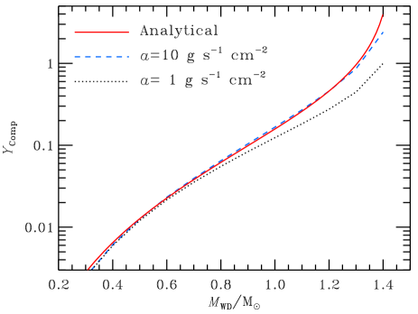
Figure 2: Dependence of the Compton parameter $Y_{\rm Comp}$ for the PSR on the WD mass. The solid curve gives the results for the analytical model (7) of Frank et al. (2002) given by Eq. (21), while the dotted and dashed curves are for the numerical model of Suleimanov et al. (2005) for two accretion rates $a$ = 1 and 10 g s^-1 cm^-2, respectively.

Figure 3: Comparison of PSR models computed for $M_{\rm wd}=1.2M_{\odot}$ with a local accretion rate $a=10$ g s^-1 cm^-2 with (solid curves) and without (dashed curves) Compton scattering taken into account. The temperature and the density structures (panel a), as well as the emergent spectra (panel b), are shown. The dotted lines correspond to the analytical solution (7).

2.4 Results of calculations

Before presenting the results of our calculations, let us first evaluate the importance of cooling by Compton scattering in the PSR. The Compton parameter

$$Y_{\rm Comp}=4\Theta\max(\tau_{\rm e},\tau_{\rm e}^{2})$$ (20)

can be calculated for various models of the PSR. The analytical model (7) yields

$$Y_{\rm Comp}=4\sigma_{\rm T}\int_{0}^{H_{\rm s}}\leavevmode\nobreak\ \Theta\leavevmode\nobreak\ n_{\rm e}\leavevmode\nobreak\ {\rm d}z=0.05\leavevmode\nobreak\ \mu^{1/2}\leavevmode\nobreak\ \mu_{\rm e}\leavevmode\nobreak\ m^{2}\leavevmode\nobreak\ R_{9}^{-2}.$$ (21)

It is clear the Compton parameter can be close to unity only for high-mass WDs. It is possible to also compute $Y_{\rm Comp}$ using numerical models of the PSRs (Suleimanov et al., 2005). The dependence of $Y_{\rm Comp}$ on the WD mass is shown in Fig. 2. We see that at high accretion rates and high WD masses, Compton scattering can affect the structure of the PSR and the emergent spectrum.

The influence of Comptonization on the temperature and the density structure of the PSR, as well as the emergent spectra, are demonstrated in Fig. 3. Here we take a 1.2 $M_{\odot}$ WD with a local accretion rate $a=10$ g s^-1 cm^-2 and compute the PSR structure with and without Comptonization taken into account. The amplification factor $1+A$ due to Compton scattering is about 1.5 at the top of the PSR (near the shock) and decreases to 1 at the WD surface. Therefore, if Comptonization is taken into account, the cooling rate becomes higher, the height of PSR smaller, and the emergent spectrum slightly harder. But the difference between the emergent spectra with and without Comptonization is, however, rather small.

We computed the grid of PSR models for WD masses ranging from 0.3 to 1.3 $M_{\odot}$ with step 0.02 $M_{\odot}$ (51 models in total). The total accretion rate was assumed to be $\dot{M}=10^{17}$ g s^-1 with the fixed part $f=10^{-3}$ of the WD surface occupied by PSR. This gives different local accretion rates $a$ for various WD masses, varying from $\sim 0.5$ to $\sim 5$ g s^-1 cm^-2. The emergent spectra of PSR with different local accretion rates (in the interval 0.1–10 g s^-1 cm^-2) are very similar (Suleimanov et al., 2005); therefore, we have only one free parameter, the WD mass, in our grid of model spectra. This means that the mass can be found by fitting the observed X-ray spectrum. Of course, the WD mass determination using spectral fitting is model dependent, because of using of the specific theoretical WD mass-radius relation and of the framework the theoretical spectra are calculated. However, the WD mass determination depends very little on the particular choice of $\dot{M}$ and $f$.

The grid of the IP spectral models has been incorporated into the XSPEC software package under the name IPCOMP and is publicly available.

3 X-ray spectrum of V709 Cas

V709 Cas is a typical IP emitting in the hard X-rays (see e.g. Suleimanov et al., 2005). The present dataset was obtained using the RXTE/PCA (3–20 keV) (Jahoda et al., 1996) and INTEGRAL/IBIS/ISGRI (20–120 keV) (Ubertini et al., 2003; Lebrun et al., 2003) instruments with the total effective exposure times of 47 ks and 4.5 Ms, respectively. Our spectral model consists of the PSR model IPCOMP, an iron line modelled as a Gaussian, and the partial absorption model PCFABS described by the covering factor $C_{\rm F}$ and the column density $N_{\rm H}$. The spectral analysis is performed with the XSPEC (Arnaud, 1996) version 12.4.

The best fit with $\chi^{2}/{\rm d.o.f.}=31/30$ is obtained for $M_{\rm wd}=0.91_{-0.02}^{+0.03}M_{\odot}$, a partial covering fraction $C_{\rm F}=0.41\pm 0.05$ and $N_{\rm H}=(53\pm 10)\times 10^{22}$ cm^-2 (see Fig. 4). The iron line energy is $6.5\pm 0.2$ keV with an equivalent width of 508 eV. The unabsorbed flux between 0.5 and 150 keV is $F\simeq 2.4\times 10^{-10}$ erg cm^-2 s^-1, which translates into a bolometric luminosity of $L\simeq 1.52\times 10^{33}$ erg s^-1, for the source distance of 230 pc (Bonnet-Bidaud et al., 2001).

We can estimate the mass accretion rate using the simple relation $\dot{M}=LR_{\rm wd}/(GM_{\rm wd})$. We get $\dot{M}=0.8\times 10^{16}$ g s^-1 for the WD radius of $R_{\rm wd}\simeq 0.61\times 10^{9}$ cm, which was computed using Eq. (10). To investigate the role of Compton scattering, we also implemented into XSPEC the grids of the PSR model without Compton scattering. The derived parameters are similar to those obtained with the Compton scattering model with a comparable reduced $\chi^{2}$. The WD mass is found to be slightly lower $M_{\rm wd}=0.88_{-0.01}^{+0.02}M_{\odot}$. This seems counter-intuitive, because Comptonization increases the flux at high energies, and therefore would need lower temperature (and therefore lower WD mass) to radiate the same energy. However, the spectral slope in the 4–20 keV energy range is different for the two models, so the absorber parameters also change to $C_{\rm F}=0.44\pm 0.05$ and $N_{\rm H}=(63\pm 10)\times 10^{22}$ cm^-2. Thus for V709 Cas, both mass estimations are consistent with each other within the errors, and Compton scattering does not have much effect, which is expected for such a WD mass and a rather low accretion rate.

For illustrative purpose, we also obtained a fit of the observed spectrum with a single temperature bremsstrahlung model. We obtained $T=29.6\pm 2.5$ keV, $C_{\rm F}=0.31\pm 0.04$, $N_{\rm H}=(58\pm 15)\times 10^{22}$ cm^-2, and the iron line energy $6.5\pm 0.2$ keV with the reduced $\chi^{2}$ = 1.062. Using a linear approximation to the mass-radius relation (11), we can estimate the WD mass:

$$m=\frac{T_{\rm keV}}{23.6+0.59T_{\rm keV}},$$ (22)

which gives $M_{\rm wd}=0.72\pm 0.035M_{\odot}$. This result illustrates the error from the use of a simple one-temperature bremsstrahlung model for the WD mass estimation.

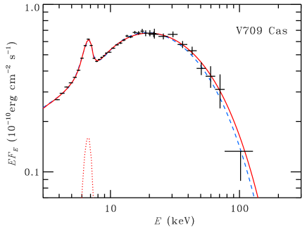
Figure 4: The unfolded spectrum of V709 Cas and the best-fit spectral model of the PSR. The crosses represent the data from RXTE/PCA (3–20 keV) and INTEGRAL/ISGRI (20-100 keV) instruments. The total spectrum of the PSR model is shown by the solid (with Compton scattering) and the dashed (without Compton scattering) curves. The dotted curve represents the Gaussian iron line.

4 Conclusions

We have studied the influence of Compton scattering on the structure of the post-shock region and the broad-band X-ray spectra of intermediate polars. Compton scattering leads to slightly harder emergent spectra and smaller PSR height. The effect can be significant for the luminous intermediate polars with high-mass WDs. We have also constructed a grid of the emergent spectra in a wide range of WD masses and incorporated into the XSPEC package. We used this grid to fit the broad-band X-ray spectrum of V709 Cas observed by RXTE and INTEGRAL observatories and determined the WD mass in this object. Accounting for Compton scattering does not change the obtained mass significantly.

In this work we have not considered the cooling by cyclotron radiation. However, for WDs with stronger magnetic field (polars), Comptonization of the cyclotron photons can significantly affect the structure of the PSR and the emergent spectra. We plan to perform such a study in the future.