Calculated magnetoresistance due to domain walls in nanostructures

Abstract

The existing Levy-Zhang approach to constructing the contribution to the resistivity of a metal of a magnetic domain wall is explored. The model equations are integrated analytically, giving a closed form expression for the resistivity when the current flows in the wall. The Boltzmann equation is solved analytically and the ratio of the spin up and spin down resistivities is calculated and its dependence on the strength of the Coulomb and exchange scattering potentials is elucidated.

I Introduction

Domain walls are examples of topological solitons in magnetism and they arise due to the competition between exchange and anisotropy energy. Domain wall motion by a spin polarized current has been gathering much interest recently mainly due to emerging device applications such as domain wall memory and domain wall logic devices. Winding number (vorticity), chirality and even skyrmion number are other degrees of freedom when considering the magnetic domain wall and this is fascinating from the point of view of fundamentals as well as information storage considerations. Understanding the mechanisms by which a magnetic domain wall contributes to the resistivity of a metal, is a problem on equal footing with that of describing how a spin polarized current imparts torque to magnetization. When a conduction band electron fails to track the lattice magnetization when traversing a domain wall, an angle is subtended between the conduction band spin and the wall, which leads to a torque and, in the presence of impurity scattering, a measurable magnetoresistance. The relationship between domain wall motion spin transfer torque and domain wall magnetoresistance was proposed by Tatara et al. Tatara and Fukuyama (1997).
In this paper, we are interested in calculating analytically the explicit formula for the contribution of a domain wall to the resistivity in the diffusive limit, using the model equations of Levy and Zhang Levy and Zhang (1997). We wish to integrate this model, giving explicit formulae for the resistivity of a domain wall and use this formalism to calculate MR curves for systems in which domain walls nucleate in nanostructures by shape anisotropy.

II Admixture states at a domain wall

We first begin with the simple picture of a 2 band ferromagnetic metal where the Fermi level lies in the Stoner split bands. We consider the Hamiltonian of a uniformly magnetized ferromagnet with the unit vector of magnetization aligned along the +z axis ($\sigma.\hat{n}=\sigma_{z}$), and so the starting SU(2) Hamiltonian takes the following form :

$$H_{0}=\frac{-\hbar^{2}\nabla^{2}}{2m^{*}}+V(\overrightarrow{r})+J\sigma_{z},$$ (1)

where m^∗ is the effective electron mass and V($\overrightarrow{r}$) is the periodic crystal potential, taken to be invariant under SU(2) rotation and therefor this does not contribute to the spin scattering in the analysis which follows. We now write the Hamiltonian H₀ in matrix form and look for eigenstates in the Hilbert space $L_{2}\otimes{\emph{H}_{s}}$.

$$H_{0}=\left(\begin{array}[]{cc}-\beta\nabla^{2}+J&0\\ 0&\beta\nabla^{2}-J\\ \end{array}\right),$$ (2)

where $\beta$ =$\hbar^{2}/(2m^{*})$. We now transform H₀ onto the basis $\{e^{i\overrightarrow{k_{\sigma}}.\overrightarrow{r}}\}$, which assumes eigenvectors of the form $\Phi_{\overrightarrow{k}\sigma}$=$e^{i\overrightarrow{k_{\sigma}}.\overrightarrow{r}}$ $\varphi_{s}$, where $\varphi_{s}$ is a two-component spinor. Writing $\hat{H}=\langle\Phi^{*}_{\overrightarrow{k}\sigma}|H_{0}|\Psi_{\overrightarrow{k}\sigma}\rangle$, we find :

$$\hat{H}=\left(\begin{array}[]{cc}\beta k_{\sigma}^{2}+J&0\\ 0&-\beta k_{\sigma}^{2}-J\\ \end{array}\right).$$ (3)

The eigenvalues of Equation 3 can be written as : $\lambda_{\pm}$ =$\beta k^{2}_{\pm}\pm J$ where the $\pm$ signs refer to pure spin eigenstates. We now write the 2 component spinors for an unperturbed 2 band, exchange split ferromagnet.

$$\phi^{(0)}_{\uparrow}=\frac{1}{\sqrt{N}}\left(\begin{array}[]{c}e^{i\overrightarrow{k_{\uparrow}}.\overrightarrow{r}}\\ 0\\ \end{array}\right),\\ \phi^{(0)}_{\downarrow}=\frac{1}{\sqrt{N}}\left(\begin{array}[]{c}0\\ e^{i\overrightarrow{k_{\downarrow}}.\overrightarrow{r}}\\ \end{array}\right),$$ (4)

which describe pure spin states characterizing a two-band ferromagnet each with eigen energies E_↑,↓ = $\beta$ k${}_{\uparrow,\downarrow}^{2}\pm J$. We now turn our attention to the perturbation associated with a magnetic domain wall (DW), where the description of the conduction band spin goes beyond that of pure spins states. If the region of space over which the magnetization in a DW rotates is comparable the length scale of the Fermi wavelength 1/k_F, there will be an adiabatic ’mistracking’ of the conduction spin with the lattice magnetization (see Fig. 1). Nevertheless, as we will see, this scaling is treated as a perturbation in the Levy-Zhang approach. The perturbation parameter is proportional to $\nabla\theta.\overrightarrow{k_{F}}$ and this is assumed to be small for the perturbation expansion to converge.

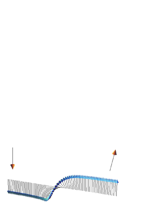
Figure 1: (Color Online) Schematic of a conduction band electron traversing a 180^o Bloch domain wall and undergoing mistracking.

We write the Hamiltonian defined in equation 1 in the transformed basis of the domain wall R${}_{\theta}\Phi^{(0)}_{\sigma}$ which gives :

$$\bar{H}=R^{-1}_{\theta}HR_{\theta}=H_{0}+R^{-1}_{\theta}[H,R_{\theta}],$$ (5)

where H₀ is now the unperturbed Hamiltonian of the magnetic system and R_θ is the SU(2) rotation operator e${}^{-i\frac{\theta}{2}\hat{n}.\sigma}$. Indeed, in the basis of pure spin states, $\theta$ is the polar angle of the magnetization unit vector $\hat{n}$. We recognize that the perturbation potential can be written from the equation above as $V_{pert}$=$R^{-1}_{\theta}[H,R_{\theta}]$. Now, R_θ commutes with the J $\hat{n}.\sigma$ and V($\overrightarrow{r}$)terms in H₀, so we are left with V_pert in the following form :

$$V_{pert}=-\beta R^{-1}_{\theta}[\nabla^{2},R_{\theta}]$$ (6)

$$=-\beta R^{-1}_{\theta}(\nabla^{2}R_{\theta}-R_{\theta}\nabla^{2})$$ (7)

$$=-\beta(R^{-1}_{\theta}\nabla^{2}R_{\theta}-\nabla^{2}).$$ (8)

Now, in order to evaluate the left hand side term of the above equation $R^{-1}_{\theta}\nabla R_{\theta}$, we act on a trial wavefunction $\psi$ from the left as follows :

$$(R^{-1}_{\theta}\nabla.\nabla R_{\theta})\psi$$ (9)

$$=R^{-1}_{\theta}\nabla(\nabla R_{\theta}\psi+R_{\theta}\nabla\psi)$$ (10)

$$=R^{-1}_{\theta}(\nabla^{2}R_{\theta}+(\nabla R_{\theta})\nabla\psi+(\nabla R_{\theta})\nabla\psi+R_{\theta}\nabla^{2}\psi)$$ (11)

$$=R^{-1}_{\theta}(\nabla^{2}R_{\theta}\psi+(\nabla R_{\theta})\nabla\psi+(\nabla R_{\theta})\nabla\psi+R_{\theta}\nabla^{2}\psi)$$ (12)

$$=(R^{-1}_{\theta}\nabla^{2}R_{\theta}+2R^{-1}_{\theta}\nabla R_{\theta}\nabla+\nabla^{2})\psi)$$ (13)

Inserting this into equation 8, we arrive at the following expression ;

$$V_{pert}=-\beta(R^{-1}_{\theta}\nabla^{2}R_{\theta}-\nabla^{2})\psi\\ =-\beta(R^{-1}_{\theta}\nabla^{2}R_{\theta}+2R^{-1}_{\theta}(\nabla R_{\theta})\nabla+\nabla^{2})\psi$$ (15)

We can can simply write $\nabla R_{\theta}=-i\frac{\nabla\theta}{2}(\hat{n}.\sigma)e^{-i\frac{\theta}{2}\hat{n}.\sigma}$ and $\nabla^{2}R_{\theta}=-\frac{|\nabla\theta|^{2}}{4}(\hat{n}.\sigma)^{2}e^{-i\frac{\theta}{2}\hat{n}.\sigma}$ - $i\frac{\nabla^{2}\theta}{2}(\hat{n}.\sigma)e^{-i\frac{\theta}{2}\hat{n}.\sigma}$ which, when substituted into V_pert now gives :

$$V_{p}=-\beta\left[-\frac{|\nabla\theta|^{2}}{4}(\hat{n}.\sigma)^{2}-i\frac{\nabla^{2}\theta}{2}(\hat{n}.\sigma)-i\nabla\theta(\hat{n}.\sigma).\nabla\right]$$ (16)

Recall that $\beta$ = $\hbar^{2}/2m^{*}$ which is just a constant and that $\theta$ is the angle of the magnetization. Recognizing that, for generators of SU(2) rotations, $(\hat{n}.\sigma)^{2}$ = 1, which means that the first term in V_pert is diagonal and so does not mix spin states. Further, if the wall magnetization is assumed to be slowly varying in space with respect to the length scale defined by $1/k_{F}$, we have $\nabla^{2}\theta/(2\nabla\theta k_{F})$ $\ll$ 1. This latter term may become important in DW profiles with vanishing $\nabla\theta$ but finite $\nabla^{2}\theta$ (i.e. a stationary point in $\theta$) which would occur in DW configurations with finite winding (n$\geq$1) or skyrmion number. As a first approximation, we retain the first order term in V_pert = -$\beta\nabla\theta(\hat{n}.\sigma)(-i\nabla)$ and use the perturbation formalism outlined in Appendix A. We write the new eigenspinors in the rotated basis as :

$$|\uparrow^{{}^{\prime}}\rangle=R_{\theta}\left(\begin{array}[]{c}e^{i\overrightarrow{k}_{\uparrow}.\overrightarrow{r}}\\ 0\\ \end{array}\right)$$ (19)

$$|\downarrow^{{}^{\prime}}\rangle=R_{\theta}\left(\begin{array}[]{c}0\\ e^{i\overrightarrow{k}_{\downarrow}.\overrightarrow{r}}\\ \end{array}\right)$$ (22)

For a Bloch wall, where the magnetization rotates in the yz plane, we now write the expansion coefficients for the first order corrections to the wavefunction (see Appendix A), as follows :

$$C^{(1)}_{k}=\displaystyle\sum_{n\neq k}\frac{V_{nk}}{E^{(0)}_{n}-E^{(0)}_{k}}$$ (23)

$$=\displaystyle\sum_{n\neq k}\frac{\langle k^{(0)}|-\beta\nabla\theta.-i\nabla(\hat{n}.\sigma)|n^{(0)}\rangle}{E^{(0)}_{n}-E^{(0)}_{k}}$$ (24)

$$=C^{(1)}_{\uparrow}=\frac{\langle\uparrow|-\beta(\nabla\theta).(-i\nabla\theta)(\hat{n}.\sigma)|\downarrow\rangle}{E^{(0)}_{\downarrow}-E^{(0)}_{\uparrow}}$$ (25)

$$=\frac{\int d^{3}\overrightarrow{r}(-i\beta\nabla\theta.\overrightarrow{k_{\downarrow}}e^{i(\overrightarrow{k}_{\uparrow}-\overrightarrow{k}_{\downarrow}).\overrightarrow{r}})}{-2J+\beta(k_{\downarrow}^{2}-k_{\uparrow}^{2})}$$ (26)

We find a similar expression for the C${}^{(1)}_{\downarrow}$ mixing coefficient. It is important to note also that the unit vector along the magnetization can be written as $\hat{n}=(0,\sin(\theta)\sin(\phi),\cos(\theta))=(0,sech(x/\lambda)\sin(\phi),\tanh(x/\lambda))$, for a Bloch wall in the +x direction with chirality $\phi$. $\lambda$ is the equilibrium wall width (=$\sqrt{(}A/K)$, A being the exchange stiffness and K is the magnetic anisotropy energy density). In this wall configuration, $\hat{n}.\sigma$ has the components $n_{y}\sigma_{2}+n_{z}\sigma_{3}$, where $\sigma_{i}$ refers to the components of the Pauli spinors. Moreover, only the $\sigma_{2}$ term yields a non-zero contribution to the mixing coefficient as it’s elements are off diagonal. If the wall is set up to rotate in the xz plane, the coefficient C⁽¹⁾ would be real.

$$C^{(1)}_{\uparrow}=\frac{\int d^{3}\overrightarrow{r}(i\beta(e^{i(-\overrightarrow{k}_{\uparrow}+\overrightarrow{k}_{\downarrow}).\overrightarrow{r}}\nabla\theta.\overrightarrow{k_{\downarrow}}+\frac{\nabla^{2}\theta}{2}e^{i(-\overrightarrow{k}_{\uparrow}+\overrightarrow{k}_{\downarrow}).\overrightarrow{r}}))}{\beta(k^{2}_{\downarrow}-k^{2}_{\uparrow})-2J}$$ (27)

$$C^{(1)}_{\downarrow}=\frac{\int d^{3}\overrightarrow{r}(-i\beta(e^{i(-\overrightarrow{k}_{\downarrow}+\overrightarrow{k}_{\uparrow}).\overrightarrow{r}}\nabla\theta.\overrightarrow{k_{\uparrow}}+\frac{\nabla^{2}\theta}{2}e^{i(-\overrightarrow{k}_{\downarrow}+\overrightarrow{k}_{\uparrow}).\overrightarrow{r}}))}{\beta(k^{2}_{\uparrow}-k^{2}_{\downarrow})+2J}$$ (28)

In ferromagnetic metals, it is reasonable to assume that the kinetic energy splitting between the bands is much smaller than the exchange splitting , this condition is written as $\frac{\beta(k^{2}_{\uparrow}-k^{2}_{\downarrow})}{2J}\ll 1$. It can further be assumed that $k^{F}_{\uparrow}\simeq k^{F}_{\downarrow}$, which is true to within an order of magnitude for most ferromagnets, and for the purposes of this calculation, the assumption is convenient in establishing the order of of magnitude of the effect. For spatially dependent $\nabla\theta$, $\nabla^{2}\theta$ and $\hat{n}(\overrightarrow{r}).\sigma$ this assumption would have to be relaxed and these terms will couple to the scattering coefficients $C^{(1)}_{\uparrow,\downarrow}$ via a transformation on the basis kets $\{|\uparrow^{{}^{\prime}}\rangle,|\downarrow^{{}^{\prime}}\rangle\}$ via :

$$\langle\uparrow^{{}^{\prime}}|i\beta\nabla\theta.\overrightarrow{k}_{\downarrow}\hat{n}(\overrightarrow{r}).\sigma\nabla|\downarrow^{{}^{\prime}}\rangle,$$ (30)

$$\langle\downarrow^{{}^{\prime}}|-i\beta\nabla\theta.\overrightarrow{k}_{\uparrow}\hat{n}(\overrightarrow{r}).\sigma\nabla|\uparrow^{{}^{\prime}}\rangle,$$ (31)

which correspond to the C${}^{(1)}_{\uparrow}$ and C${}^{(1)}_{\downarrow}$ mixing coefficients, respectively. We now write the total wavefunction of the electron in terms of the adiabatically mixed two component spinors in the rotated basis, as follows :

$$|\Psi_{\uparrow}^{{}^{\prime}}\rangle=\frac{1}{\sqrt{N}}\left[R_{\theta}\left(\begin{array}[]{c}e^{i\overrightarrow{k}_{\uparrow}.\overrightarrow{r}}\\ 0\\ \end{array}\right)+C^{(1)}_{\uparrow}R_{\theta}\left(\begin{array}[]{c}0\\ e^{i\overrightarrow{k}_{\uparrow}.\overrightarrow{r}}\\ \end{array}\right)\right]$$ (36)

$$|\Psi_{\downarrow}^{{}^{\prime}}\rangle=\frac{1}{\sqrt{N}}\left[R_{\theta}\left(\begin{array}[]{c}0\\ e^{i\overrightarrow{k}_{\downarrow}.\overrightarrow{r}}\\ \end{array}\right)+C^{(1)}_{\downarrow}R_{\theta}\left(\begin{array}[]{c}e^{i\overrightarrow{k}_{\downarrow}.\overrightarrow{r}}\\ 0\\ \end{array}\right)\right]$$ (41)

Using the approximations implemented by Levy and Zhang, we can write $C^{(1)}_{\uparrow}=-i\frac{k_{x}\xi}{k_{F}}$ and $C^{(1)}_{\downarrow}=i\frac{k_{x}\xi}{k_{F}}$ for a wall whose magnetization rotates along the x-axis in the adopted coordinate system. We now define the ’spin mistracking’ parameter as :

$$\xi=\frac{\beta\nabla\theta.\overrightarrow{k_{F}}}{2J}$$ (42)

Here $\nabla\theta$ is the local magnetization angle gradient, which can be taken to be locally constant. The normalization coefficients, can be written as follows ; $N_{\sigma}=\|\Psi^{{\dagger}}_{\sigma}\Psi_{\sigma}\|=1$, we find that N(k_x)= $1+(\frac{k_{x}\xi}{k_{F}})^{2}$. The value of $\nabla\theta$ can be taken to be locally constant over the lengthscale 1/k_F and for linearly varying magnetization profiles, the mistracking can be written as

$$\xi=\frac{\hbar^{2}k_{F}\pi}{4mJD}$$ (43)

which describes mistracking at the wall whose profile is - $\theta(x)=\frac{\pi x}{D}$ (-D$<$x$<$D), originally considered by Levy and Zhang. We now write the corrections to the total wavefunction to first order as

$$|\Psi_{\uparrow}^{{}^{\prime}}(\overrightarrow{k},\overrightarrow{r})\rangle=\frac{1}{1+(\frac{\xi k_{x}}{k_{F}})^{2}}\left[R_{\theta}\left(\begin{array}[]{c}e^{i\overrightarrow{k}_{\uparrow}.\overrightarrow{r}}\\ i\frac{k_{x}\xi}{k_{F}}e^{i\overrightarrow{k}_{\uparrow}.\overrightarrow{r}}\\ \end{array}\right)\right]$$ (46)

$$|\Psi_{\downarrow}^{{}^{\prime}}(\overrightarrow{k},\overrightarrow{r})\rangle=\frac{1}{1+(\frac{\xi k_{x}}{k_{F}})^{2}}\left[R_{\theta}\left(\begin{array}[]{c}-i\frac{k_{x}\xi}{k_{F}}e^{i\overrightarrow{k}_{\downarrow}.\overrightarrow{r}}\\ e^{i\overrightarrow{k}_{\downarrow}.\overrightarrow{r}}\\ \end{array}\right)\right]$$ (49)

III Impurity scattering at a domain wall

The domain wall itself does not necessarily give rise to inelastic scattering or to a measurable resistance. However, let us consider what happens when we consider an impurity potential to which the conduction spin is coupled via the coulomb and exchange interaction. The scattering potential is defined as follows :

$$V_{scatt}(\overrightarrow{r})=\displaystyle\sum_{i}\left[v+j\sigma.\hat{M}(\overrightarrow{r}_{i})\right]\delta(\overrightarrow{r}-\overrightarrow{r}_{i})$$ (50)

This scattering potential has the following matrix elements in the basis $\{|\Psi_{\sigma}(\overrightarrow{r})\rangle\}$ as follows :

$$V^{\sigma\sigma^{{}^{\prime}}}_{kk^{{}^{\prime}}}=\displaystyle\int d^{3}\overrightarrow{r}\Psi^{{\dagger}}_{\sigma}(\overrightarrow{k},\overrightarrow{r})V_{scatt}\Psi_{\sigma^{{}^{\prime}}}(\overrightarrow{k^{\prime}},\overrightarrow{r}).$$ (51)

Using the basis defined by equation 49, we write down the matrix elements of the scattering potential :

$$V^{\uparrow\uparrow}_{kk^{{}^{\prime}}}=\displaystyle\sum_{i}\int\frac{1}{N(k)N(k^{{}^{\prime}})}R^{-1}_{\theta}\left(\begin{array}[]{cc}e^{-i{\bf k}_{\uparrow}.\overrightarrow{r}}&C^{*(1)}_{\uparrow}e^{-i{\bf k}_{\uparrow}.\overrightarrow{r}}\\ \end{array}\right).$$ (53)

$$\left[R_{\theta}v\left(\begin{array}[]{c}e^{i{\bf k}^{{}^{\prime}}_{\uparrow}.\overrightarrow{r}}\\ C^{(1)}_{\uparrow}e^{i{\bf k}^{{}^{\prime}}_{\uparrow}.\overrightarrow{r}}\\ \end{array}\right)+j\sigma.\hat{M}(\overrightarrow{r}_{i})R_{\theta}\left(\begin{array}[]{c}e^{i{\bf k}^{{}^{\prime}}_{\uparrow}.\overrightarrow{r}}\\ C^{(1)}_{\uparrow}e^{i{\bf k}^{{}^{\prime}}_{\uparrow}.\overrightarrow{r}}\\ \end{array}\right)\right]\delta(\overrightarrow{r}-\overrightarrow{r}_{i})d^{3}\overrightarrow{r}$$ (58)

Note : $|\displaystyle\sum_{i}e^{i({\bf k^{{}^{\prime}}}-{\bf k}).r_{i}}|^{2}=\displaystyle\sum_{i,j}e^{i({\bf k}^{{}^{\prime}}-{\bf k}).{\bf r}_{i}}e^{i({\bf k}^{{}^{\prime}}-{\bf k}).{\bf r_{j}}}=\displaystyle\sum_{i}1+\displaystyle\sum_{i\neq j}e^{i({\bf k}^{{}^{\prime}}-{\bf k}).({\bf r_{i}}-{\bf r}_{j})}=c_{i}\Omega$ ,where c_i refers to the concentration of impurity scattering sites. This counting is an average over all of the impurity sites and each site is taken to be equivalent. Having established the matrix elements of the scattering potential, we write down the scattering rates based on Fermi’s golden rule. After integration, the scattering matrix elements can be written in the following form :

$$\|V^{\uparrow\uparrow}_{kk^{{}^{\prime}}}\|^{2}=c_{i}\frac{1}{N^{2}(k_{x})N^{2}(k^{{}^{\prime}}_{x})}\left[(v+\sigma j)+\frac{k_{x}k^{{}^{\prime}}_{x}}{k^{2}_{F}}\xi^{2}(v-\sigma j)\right]^{2}$$ (59)

$$\|V^{\uparrow\downarrow}_{kk^{{}^{\prime}}}\|^{2}=c_{i}\frac{1}{N^{2}(k_{x})N^{2}(k^{{}^{\prime}}_{x})}\left[(v+j)k^{{}^{\prime}}_{x}-(v-j)k_{x}\right]^{2}\frac{\xi^{2}}{k^{2}_{F}}$$ (60)

$$W^{\sigma\sigma^{{}^{\prime}}}_{kk^{{}^{\prime}}}=\frac{2\pi}{\hbar}\delta(\epsilon_{{\bf k}\sigma}-\epsilon_{{\bf k}^{{}^{\prime}}\sigma})\|V^{\sigma\sigma^{{}^{\prime}}}_{kk^{{}^{\prime}}}\|^{2}.$$ (61)

$$W^{\sigma\sigma}_{{\bf kk^{{}^{\prime}}}}=\frac{2\pi}{\hbar}c_{i}\frac{1}{N^{2}(k_{x})N^{2}(k^{{}^{\prime}}_{x})}\left[(v+\sigma j)+\frac{k_{x}k^{{}^{\prime}}_{x}}{k^{2}_{F}}\xi^{2}(v-\sigma j)\right]^{2}$$ (62)

$$W^{\sigma\sigma^{{}^{\prime}}}_{kk^{{}^{\prime}}}=\frac{2\pi}{\hbar}c_{i}\frac{1}{N^{2}(k_{x})N^{2}(k^{{}^{\prime}}_{x})}\left[(v+j)k^{{}^{\prime}}_{x}-(v-j)k_{x}\right]^{2}\frac{\xi^{2}}{k^{2}_{F}}$$ (63)

These scattering rates can be integrated over momentum space (${\bf k}^{{}^{\prime}}$ coordinates) in order to find the total scattering lifetimes for momentum states within a spin channel and for momentum scattering which mixes the spin channels. This total scattering rate is defined as follows :

$$[\tau^{\sigma}({\bf k})]^{-1}=\frac{1}{(2\pi)^{3}}\displaystyle\int d^{3}{\bf k}^{{}^{\prime}}(W^{\sigma\sigma}_{{\bf kk}^{{}^{\prime}}}+W^{\sigma\sigma}_{{\bf kk}^{{}^{\prime}}})$$ (64)

$$[\tau^{\sigma}({\bf k})]^{-1}=\frac{1}{(2\pi)^{3}}\displaystyle\int d^{3}{\bf k}N^{-2}(k_{x})N^{-2}(k^{{}^{\prime}}_{x})$$

$$\left[((v+j)k^{{}^{\prime}}_{x}-(v-j)k_{x})^{2}\frac{\xi}{k^{2}_{F}}+((v+\sigma j)+\frac{k_{x}k^{{}^{\prime}}_{x}}{k^{2}_{F}}\xi^{2}(v-\sigma j))\right]^{2}\delta(\epsilon_{{\bf k}\sigma}-\epsilon_{{\bf k}^{{}^{\prime}}\sigma}).$$

We expand the normalization constants $N(k_{x})$ to second order $\xi$ as follows ; $N^{-2}(k_{x})\simeq 1-(\frac{k_{x}\xi}{k_{F}})^{2}+O((\frac{k_{x}\xi}{k_{F}})^{4})$ and we apply this approximation in order to evaluate the integral in Equation III. Recognizing that Equation III has integrals of two types, we define these two types as follows ;

$$I_{1}=\frac{2\pi c_{i}}{\hbar}\displaystyle\int d^{{}^{\prime}}k^{3}\frac{\xi^{2}}{k^{2}_{F}}(Ak^{{}^{\prime}}_{x}+B)^{2}(1-2\frac{(k_{x}k^{{}^{\prime}}_{x})^{2}}{k^{2}_{F}}\xi^{2}+..)\delta(\epsilon_{{\bf k}\sigma}-\epsilon_{{\bf k}^{{}^{\prime}}\sigma})$$ (65)

$$I_{2}\frac{2\pi c_{i}}{\hbar}\displaystyle\int d^{{}^{\prime}}k^{3}\frac{\xi^{2}}{k^{2}_{F}}(C+D\frac{k^{{}^{\prime}}_{x}\xi^{2}}{k^{2}_{F}})^{2}(1-2\frac{(k_{x}k^{{}^{\prime}}_{x})^{2}}{k^{2}_{F}}\xi^{2}+..)\delta(\epsilon_{{\bf k}\sigma}-\epsilon_{{\bf k}^{{}^{\prime}}\sigma}),$$ (66)

where we define the following constants within the integral.

$$A=(v+j),\\ B=-(v-j)k_{x},\\ C=(v+\sigma j),\\ D=k_{x}(v-\sigma j).$$

The k space volume element is given in spherical polar coordinates as $d^{3}{\bf k}$ = $k^{2}\sin(\theta)\cos(\phi)dk$ and we write down I₁ using this coordinate system, while expanding to second order in $\xi$, as follows :

$$\begin{array}[]{c}I_{1}=\frac{2\pi c_{i}}{\hbar}\displaystyle\int d^{{}^{\prime}}kk^{{}^{\prime}2}\sin(\theta)d\phi d\theta\frac{\xi^{2}}{k^{2}_{F}}(Ak^{{}^{\prime}}\sin\theta^{{}^{\prime}}\cos\phi^{{}^{\prime}}+B)^{2}\times\\ (1-2k^{2}_{x}k^{{}^{\prime}2}\sin^{2}\theta^{{}^{\prime}}\cos^{2}\phi^{{}^{\prime}}\frac{\xi^{2}}{k^{2}_{F}}+..)\delta(\epsilon_{{\bf k}\sigma}-\epsilon_{{\bf k}^{{}^{\prime}}\sigma}).\\ \displaystyle\int d^{{}^{\prime}}kk^{{}^{\prime}2}\sin(\theta)d\phi d\theta\frac{\xi^{2}}{k^{2}_{F}}(A^{2}k^{{}^{\prime}2}\sin^{2}\theta^{{}^{\prime}}\cos^{2}\phi^{{}^{\prime}}+2ABk^{{}^{\prime}}\sin\theta^{{}^{\prime}}\cos\phi^{{}^{\prime}}+B^{2})\times\\ (1-2k^{2}_{x}k^{{}^{\prime}2}\sin^{2}\theta^{{}^{\prime}}\cos^{2}\phi^{{}^{\prime}}\frac{\xi^{2}}{k^{2}_{F}}+..)\delta(\epsilon_{{\bf k}\sigma}-\epsilon_{{\bf k}^{{}^{\prime}}\sigma}).\end{array}$$ (72)

We keep the approximation that the dimensionless mistracking is small such that $\frac{k_{x}\xi^{4}k^{{}^{\prime}}_{x}}{k^{4}_{F}}\ll 1$, and write the integral as ;

$$I_{1}=\frac{2\pi c_{i}}{\hbar}\displaystyle\int d^{{}^{\prime}}kk^{{}^{\prime}2}\delta(\epsilon_{{\bf k}\sigma}-\epsilon_{{\bf k^{\prime}}\sigma^{\prime}})d^{{}^{\prime}}\theta d^{{}^{\prime}}\phi^{{}^{\prime}}\frac{\xi^{2}}{k^{2}_{F}}\\ \left(A^{2}k^{{}^{\prime}2}\sin^{3}\theta^{{}^{\prime}}\cos^{2}\phi^{{}^{\prime}}+2AB\sin^{2}\theta^{{}^{\prime}}\cos\phi^{{}^{\prime}}+B^{2}\sin\theta^{{}^{\prime}}\right)$$ (73)

We now evaluate the integrals over k-space angle, as these are known analytically, as follows :

$$I_{1}=\frac{2\pi c_{i}}{\hbar}\displaystyle\int d^{{}^{\prime}}kk^{{}^{\prime}2}\delta(\epsilon_{{\bf k}\sigma}-\epsilon_{{\bf k^{\prime}}\sigma^{\prime}})d^{{}^{\prime}}\theta d^{{}^{\prime}}\phi^{{}^{\prime}}\frac{\xi^{2}}{k^{2}_{F}}\left(A^{2}k^{{}^{\prime}2}\frac{4\pi}{3}+2AB\pi.0+B^{2}.0\right)$$ (74)

which gives the result for $I_{1}$ and this becomes, upon substitution for A ;

$$I_{1}=\frac{k^{4}\xi^{2}4\pi(v+j)^{2}}{3k^{2}_{F}},$$ (75)

to order $\xi^{4}$. The integral of the term $\delta(\epsilon_{{\bf k}\sigma}-\epsilon_{{\bf k^{\prime}}\sigma^{\prime}})$ is constant with k-space polar angles as the band energy in the simplest case depends only on $|{\bf k}|^{2}$ and there is only a non-zero contribution to the integral for $\delta(\epsilon_{{\bf k}\sigma}-\epsilon_{{\bf k^{\prime}}\sigma^{\prime}})=\delta(\beta(k^{{}^{\prime}2}-k^{2})+(\sigma-\sigma^{{}^{\prime}})J)$, in the case where we have ${\bf k}^{{}^{\prime}}$ =${\bf k}$ and $\sigma^{{}^{\prime}}=\sigma$. We turn our attention now to the integral $I_{2}$, which can be written as :

$$\begin{array}[]{c}I_{2}=\frac{2\pi c_{i}}{\hbar}\displaystyle\int dk^{{}^{\prime}}k^{{}^{\prime}2}\delta(\epsilon_{{\bf k}\sigma}-\epsilon_{{\bf k^{\prime}}\sigma^{\prime}})d\theta^{{}^{\prime}}.\\ d\phi^{{}^{\prime}}\left(C^{2}\sin\theta^{{}^{\prime}}+2CD\frac{\sin^{2}\theta^{{}^{\prime}}\cos\phi^{{}^{\prime}}k^{{}^{\prime}}_{x}\xi^{2}}{k^{2}_{F}}+\frac{k^{{}^{\prime}2}\sin^{3}\theta^{{}^{\prime}}\cos^{2}\phi^{{}^{\prime}}D^{2}\xi^{4}}{k^{2}_{F}}\right)\left(1-2\frac{(k_{x}k^{{}^{\prime}}_{x})^{2}}{k^{2}_{F}}\xi^{2}+..\right)\end{array}$$ (78)

$$\begin{array}[]{c}I_{2}=\frac{2\pi c_{i}}{\hbar}\displaystyle\int dk^{{}^{\prime}}k^{{}^{\prime}2}\delta(\epsilon_{{\bf k}\sigma}-\epsilon_{{\bf k^{\prime}}\sigma^{\prime}})d\theta^{{}^{\prime}}d\phi^{{}^{\prime}}\\ .\left(C^{2}\sin\theta^{{}^{\prime}}-C^{2}\sin^{3}\theta^{{}^{\prime}}\cos^{2}\phi^{{}^{\prime}}\frac{2(k_{x}k^{{}^{\prime}}_{x})^{2}}{k^{2}_{F}}\xi^{2}+2CD\frac{\sin^{2}\theta^{{}^{\prime}}\cos\phi^{{}^{\prime}}k^{{}^{\prime}}_{x}\xi^{2}}{k^{2}_{F}}\right)\\ -\left(\frac{k^{{}^{\prime}2}\sin^{3}\theta^{{}^{\prime}}\cos^{2}\phi^{{}^{\prime}}C^{2}\xi^{4}}{k^{2}_{F}}-4k^{{}^{\prime}3}DC\sin^{4}\theta^{{}^{\prime}}\cos^{3}\phi^{{}^{\prime}}k^{2}_{x}\frac{\xi}{k^{4}_{F}}\right)\end{array}$$ (79)

Evaluating these integrals over k space spherical polar angles, we now have :

$$\begin{array}[]{c}I_{2}=\frac{2\pi c_{i}}{\hbar}\displaystyle\int dk^{{}^{\prime}}k^{{}^{\prime}2}\delta(\epsilon_{{\bf k}\sigma}-\epsilon_{{\bf k^{\prime}}\sigma^{\prime}})d\theta^{{}^{\prime}}d\phi^{{}^{\prime}}\\ .\left(C^{2}.0-C^{2}\frac{4\pi}{3}\frac{2(k_{x}k^{{}^{\prime}}_{x})^{2}}{k^{2}_{F}}\xi^{2}+2CD\frac{\frac{\pi.0}{2}k^{{}^{\prime}}_{x}\xi^{2}}{k^{2}_{F}}-\frac{k^{{}^{\prime}2}\frac{4\pi}{3}C^{2}\xi^{4}}{k^{2}_{F}}-4k^{{}^{\prime}3}DC\frac{3\pi.0}{8}k^{2}_{x}\frac{\xi}{k^{4}_{F}}\right)\end{array}$$ (80)

Integrating over k${}^{{}^{\prime}}$ and substituting in the definitions for C and D, we have :

$$\frac{2\pi c_{i}}{\hbar}k^{2}\left(-\frac{(v+\sigma j)^{2}8\pi\xi^{2}k^{2}k^{2}_{x}}{3k^{2}_{F}}\right)=-k^{4}\frac{2\pi c_{i}}{\hbar}(v+\sigma j)^{2}\frac{8\pi}{3}\frac{k^{2}_{x}\xi^{2}}{k^{2}_{F}}$$ (81)

We are now in a position to write down the total spin dependent scattering time as

$$[\tau^{\sigma}(\overrightarrow{k})]^{-1}=\frac{2\pi c_{i}}{\hbar}\left(\frac{k^{4}\xi^{2}4\pi(v+j)^{2}}{3k^{2}_{F}}-\frac{k^{2}k^{2}_{x}\xi^{2}8\pi(v+\sigma j)^{2}}{3k^{2}_{F}}\right)$$ (82)

The equation above defines the momentum scattering time for the spin channel $\sigma$=$\pm$ which refers to pure spins states. This is now used to solve the Blotzmann equation for the non-equilibrium distribution of electronic momentum which gives rise to the spin dependent diffusive current.

IV Analytical expression for DW conductivity

We start by finding the appropriate distribution function for the electrons in the metal, by writing down the first order solution to the Boltzmann equation as $f^{(}{\bf k},t)=f^{\sigma}({\bf k}-\frac{e{\bf E}}{\hbar}t)$. This is the distribution function for electrons in a field and the rate of change of this distribution function is given by :

$$\left(\frac{\partial f}{\partial t}\right)_{field}=\frac{\partial{\bf k}}{\partial t}.\nabla_{{\bf k}}f^{\sigma}({\bf k})=\frac{-e{\bf E}}{\hbar}.\nabla_{{\bf k}}f^{\sigma}(\epsilon_{{\bf k}})$$ (83)

To first order in the electric field (E, with the convention e$<$0), we can write $f^{\sigma}({\bf k})=f_{0}(\epsilon_{{\bf k}\sigma})$, which simply corresponds to the Fermi-Dirac distribution and we now expand the last term in the Equation 83 above, as follows ;

$$\nabla_{{\bf k}}f^{\sigma}(\epsilon_{{\bf k}})=\frac{df_{0}}{d\epsilon_{{\bf k}\sigma}}\nabla\epsilon_{{\bf k}\sigma}$$ (84)

$$=-\hbar{\bf v}^{\sigma}_{{\bf k}\sigma}\delta(\epsilon_{F}-\epsilon_{{\bf k}\sigma}),$$ (85)

which gives us the field term in the distribution function rate equation :

$$\left(\frac{\partial f}{\partial t}\right)_{field}=+e{\bf v}^{\sigma}_{\bf k}.{\bf E}\delta(\epsilon_{F}-\epsilon_{{\bf k}\sigma}).$$ (86)

We now turn our attention to the collision terms in the first order time derivative of the distribution function, and we begin with the spinless version :

$$\left(\frac{\partial f}{\partial t}\right)_{coll}=\displaystyle\sum_{{\bf k}^{{}^{\prime}}}\left(W_{{\bf k}^{{}^{\prime}}{\bf k}}f({\bf k}^{{}^{\prime}})[1-f({\bf k})]-W_{{\bf k}{\bf k}^{{}^{\prime}}}f({\bf k})[1-f({\bf k}^{{}^{\prime}})]\right).$$ (87)

where $W_{{\bf k}^{{}^{\prime}}{\bf k}}$ are the scattering rates (in units of energy per unit time). The first term in the equation above represents the ’scattering in’ terms, while the second represents the ’scattering out’ terms and for elastic scattering, we have $W_{{\bf k}{\bf k}^{{}^{\prime}}}=W_{{\bf k}^{{}^{\prime}}{\bf k}}$ which arises due to the time-reversal symmetry which inelastic processes obey.

$$\left(\frac{\partial f}{\partial t}\right)_{coll}=\displaystyle\sum_{{\bf k}^{{}^{\prime}}}W_{{\bf k}{\bf k}^{{}^{\prime}}}[f({\bf k}^{{}^{\prime}})-f({\bf k})]$$ (88)

$$\frac{\Omega}{8\pi^{3}}\displaystyle\int d^{3}{\bf k}^{{}^{\prime}}W_{{\bf k}{\bf k}^{{}^{\prime}}}[f({\bf k}^{{}^{\prime}})-f({\bf k})]$$ (89)

Now we recast these equations in spin-dependent form, and now write the collision term, as follows ;

$$\left(\frac{\partial f^{\sigma}}{\partial t}\right)_{coll}=\frac{\Omega}{8\pi^{3}}\displaystyle\int d^{3}{\bf k}^{{}^{\prime}}\left(W^{\sigma\sigma}_{{\bf k}{\bf k}^{{}^{\prime}}}[f^{\sigma}({\bf k}^{{}^{\prime}})-f^{\sigma}({\bf k})]+W^{\sigma-\sigma}_{{\bf k}{\bf k}^{{}^{\prime}}}[f^{-\sigma}({\bf k}^{{}^{\prime}})-f^{\sigma}({\bf k})]\right)$$ (90)

and we invoke the steady-state condition :

$$\left(\frac{\partial f^{\sigma}}{\partial t}\right)_{field}+\left(\frac{\partial f^{\sigma}}{\partial t}\right)_{coll}=0.$$ (91)

We now arrive at the appropriate Boltzmann equation for the spin dependent transport of electrons in the metal, in the most general sense :

$$+e{\bf v}^{\sigma}_{{\bf k}}.{\bf E}\delta(\epsilon_{F}-\epsilon_{{\bf k}\sigma})=\frac{\Omega}{8\pi^{3}}\displaystyle\int d^{3}{\bf k}\left(W^{\sigma\sigma}_{{\bf k}^{{}^{\prime}}k}[f^{\sigma}({\bf k})-f^{\sigma}({\bf k^{\prime}})]+W^{\sigma-\sigma}_{{\bf k}{\bf k}^{{}^{\prime}}}[f^{\sigma}({\bf k})-f^{-\sigma}({\bf k^{\prime}})]\right)$$ (92)

$$+e{\bf v}^{\sigma}_{{\bf k}}.{\bf E}\delta(\epsilon_{F}-\epsilon_{{\bf k}\sigma})=\frac{\Omega}{8\pi^{3}}\frac{2\pi}{\hbar}\displaystyle\int d^{3}{\bf k}|V^{\sigma\sigma}_{{\bf k}^{{}^{\prime}}k}|^{2}[f^{\sigma}({\bf k})-f^{\sigma}({\bf k^{\prime}})]\delta(\epsilon_{{\bf k}\sigma}-\epsilon_{{\bf k}^{{}^{\prime}}\sigma})+$$ (93)

$$|V^{\sigma-\sigma}_{{\bf k}{\bf k}^{{}^{\prime}}}|^{2}[f^{\sigma}({\bf k})-f^{-\sigma}({\bf k^{\prime}})]\delta(\epsilon_{{\bf k}\sigma}-\epsilon_{{\bf k}^{{}^{\prime}}-\sigma})$$ (94)

Now, for a two-band ferromagnet, we have the following relations for intra-spin-band and inter-spin-band scattering, respectively, as follows :

$$\epsilon_{{\bf k}\sigma}-\epsilon_{{\bf k}^{{}^{\prime}}\sigma}=\frac{\hbar^{2}}{2m^{*}}\left(k^{2}-k^{{}^{\prime}2}\right)$$ (95)

$$\epsilon_{{\bf k}\sigma}-\epsilon_{{\bf k}^{{}^{\prime}}-\sigma}=\frac{\hbar^{2}}{2m^{*}}\left(k^{2}-k^{{}^{\prime}2}\right)+2\sigma J$$ (96)

We also expand the Boltzmann distribution about the Fermi energy and write the non-equilibrium distribution function for the electrons as follows :

$$f^{\sigma}({\bf k})=f_{0}(\epsilon_{{\bf k}\sigma})+n^{\sigma}({\bf k})\delta(\epsilon_{F}-\epsilon_{{\bf k}\sigma})$$ (97)

$$\frac{\Omega}{4\pi^{2}}\displaystyle\int d^{3}{\bf k}|V^{\sigma\sigma}_{{\bf k}^{{}^{\prime}}k}|^{2}[n^{\sigma}({\bf k})\delta(\epsilon_{F}-\epsilon_{{\bf k}^{{}^{\prime}}\sigma})-n^{\sigma}({\bf k^{{}^{\prime}}})\delta(\epsilon_{F}-\epsilon_{{\bf k}^{{}^{\prime}}\sigma})]\delta(\epsilon_{{\bf k}\sigma}-\epsilon_{{\bf k}^{{}^{\prime}}\sigma})+$$ (98)

$$|V^{\sigma-\sigma}_{{\bf k}{\bf k}^{{}^{\prime}}}|^{2}[n^{\sigma}({\bf k})\delta(\epsilon_{F}-\epsilon_{{\bf k}^{{}^{\prime}}\sigma})-n^{-\sigma}({\bf k^{{}^{\prime}}})\delta(\epsilon_{F}-\epsilon_{{\bf k}^{{}^{\prime}}-\sigma})]\delta(\epsilon_{{\bf k}\sigma}-\epsilon_{{\bf k}^{{}^{\prime}}-\sigma})$$ (99)

$$+e{\bf v}^{\sigma}_{{\bf k}}.{\bf E}=\frac{\Omega}{4\pi^{2}}\displaystyle\int d^{3}{\bf k}|V^{\sigma\sigma}_{{\bf k}^{{}^{\prime}}k}|^{2}[n^{\sigma}({\bf k})-n^{\sigma}({\bf k^{{}^{\prime}}})]\delta(\epsilon_{F}-\epsilon_{{\bf k}^{{}^{\prime}}\sigma})+$$ (100)

$$|V^{\sigma-\sigma}_{{\bf k}{\bf k}^{{}^{\prime}}}|^{2}[n^{\sigma}({\bf k})-n^{-\sigma}({\bf k^{{}^{\prime}}})]\delta(\epsilon_{F}-\epsilon_{{\bf k}^{{}^{\prime}}-\sigma})$$ (101)

For the conductivity in the ”current in wall” geometry, we solve the Boltzmann equation with the following distribution function :

$$f^{\sigma}({\bf k})=f^{o}({\bf k})-ev^{\sigma}_{y}\delta(\epsilon_{F}-\epsilon_{{\bf k}\sigma})\tau^{\sigma}({\bf k})\\$$ (102)

and write the total conductivity $\sigma_{CIW}=\displaystyle\sum_{\sigma}\int-ef^{\sigma}({\bf k}){\bf v_{\sigma}}d^{3}{\bf k}$ of the system as

$$\sigma_{CIW}=\displaystyle\int d^{3}{\bf k}\left(-e^{2}v^{\uparrow}_{y}E\delta(E_{F}-E_{{\bf k}\uparrow})\tau^{\uparrow}({\bf k})-e^{2}v^{\downarrow}_{y}\delta(E_{F}-E_{{\bf k}\downarrow})\tau^{\downarrow}({\bf k})+f^{o}({\bf k})e(v^{\uparrow}_{y}+v^{\downarrow}_{y})\right)$$ (103)

The first two terms in the above equation are the spin dependant conductivities $\sigma_{\uparrow}$ and $\sigma_{\downarrow}$ respectively, while the last term is just the total conductivity of the two spin channels without spin relaxation.
Takin the expressions for the total scattering rates from Equation 63, we set the scattering in momentum component k_x to zero (the current is ’in wall’) and write the the total spin relaxation time as :

$$\begin{array}[]{c}[\tau({\bf k})]^{-1}=\frac{2\pi c_{i}}{(2\pi)^{3}\hbar}\displaystyle\int dk^{{}^{\prime}3}N^{2}(k_{x})\delta(\epsilon_{k\sigma}-\epsilon_{k^{{}^{\prime}}\sigma})\left[(v+\sigma j)^{2}+(v+j)^{2}k^{{}^{\prime}2}_{x}\frac{\xi^{2}}{k^{2}_{F}}\right]\\ =\frac{c_{i}}{4\pi^{2}\hbar}\displaystyle\int dk^{{}^{\prime}}k^{{}^{\prime}2}\delta(\epsilon_{k\sigma}-\epsilon_{k^{{}^{\prime}}\sigma})\\ \left(\sin\theta^{{}^{\prime}}(v+\sigma j)^{2}-(v+\sigma j)^{2}k^{{}^{\prime}2}\sin^{3}\theta^{{}^{\prime}}\cos^{2}\phi^{{}^{\prime}}\frac{\xi^{2}}{k^{2}_{F}}+(v+j)^{2}k^{{}^{\prime}2}\sin^{3}\theta^{{}^{\prime}}\cos^{2}\phi^{{}^{\prime}}\frac{\xi^{2}}{k^{2}_{F}}\right)d\theta^{{}^{\prime}}d\phi^{{}^{\prime}}\\ =\frac{c_{i}}{4\pi^{2}\hbar}\displaystyle\int dk^{{}^{\prime}}k^{{}^{\prime}2}\delta(\epsilon_{k\sigma}-\epsilon_{k^{{}^{\prime}}\sigma})\left(4\pi(v+\sigma j)^{2}-(v+\sigma j)^{2}k^{{}^{\prime}2}\frac{4\pi}{3}\frac{\xi^{2}}{k^{2}_{F}}+(v+j)^{2}k^{{}^{\prime}2}\frac{4\pi}{3}\frac{\xi^{2}}{k^{2}_{F}}\right)\\ =\frac{c_{i}}{4\pi^{2}\hbar}\left(k^{2}(4\pi(v+\sigma j)^{2}-(v+\sigma j)^{2}k^{2}\frac{4\pi}{3}\frac{\epsilon^{2}}{k^{2}_{F}}+(v+j)^{2}\frac{k^{2}\epsilon^{2}4\pi}{3k^{2}_{F}})\right).\end{array}$$

We now solve the Boltzmann equation, which is written as follows :

$$-e{\bf v}^{\sigma}.{\bf E}\delta(\epsilon_{F}-\epsilon_{{\bf k}\sigma})=\frac{1}{8\pi^{3}}\displaystyle\int W^{\sigma\sigma}_{\bf kk^{{}^{\prime}}}\left[f^{\sigma}({\bf k})-f^{\sigma}({\bf k^{{}^{\prime}}})\right]d^{3}{\bf k^{{}^{\prime}}}+\frac{1}{8\pi^{3}}\displaystyle\int W^{\sigma-\sigma}_{\bf kk^{{}^{\prime}}}\left[f^{\sigma}({\bf k})-f^{-\sigma}({\bf k^{{}^{\prime}}})\right]d^{3}{\bf k^{{}^{\prime}}}$$ (105)

which, for the geometry under consideration, we write the solution to the Boltzmann equation as $f^{\sigma}({\bf k})=f_{0}({\bf k})-ev^{\sigma}_{y}E\delta(\epsilon_{F}-\epsilon_{{\bf k}\sigma})\tau^{\sigma}({\bf k})$, which is justified as integration over ${\bf k^{{}^{\prime}}}$ results in the vanishing of scattering in ${\bf k}$ components. We use this solution to write the conductivity of the wall with the current flowing ’in wall’ $\sigma_{CIW}$.

$$\sigma_{CIW}=\sigma_{0}+\displaystyle\sum_{\sigma}\int\frac{-e^{2}\frac{\hbar^{2}}{m^{*2}}k_{\sigma}^{2}\sin^{2}\theta\sin^{2}\phi E\delta(\epsilon_{F}-\epsilon_{{\bf k}\sigma})\sin\theta k^{2}dkd\theta d\phi}{\frac{c_{i}}{4\pi^{2}\hbar}\left(4\pi k^{2}(v+\sigma j)^{2}-(v+\sigma j)^{2}\frac{4\pi k^{4}\xi^{2}}{3k^{2}_{F}}+(v+j)^{2}\frac{k^{4}\xi^{2}4\pi}{3k^{2}_{F}}\right)}\\$$ (106)

We now find that the total conductivity can be written as:

$$\begin{array}[]{c}\sigma_{CIW}=\sigma_{0}-\frac{4\pi e^{2}\frac{\hbar^{2}}{m^{*2}}}{\frac{c_{i}}{4\pi^{2}\hbar}}\left(\frac{k^{\uparrow 2}_{F}}{4\pi k^{\uparrow 2}_{F}(v+j)^{2}-(v+j)^{2}\frac{4\pi k^{\uparrow 4}_{F}\xi^{2}}{k^{2}_{F}}+(v+j)^{2}\frac{4\pi k^{\uparrow 4}_{F}\xi^{2}}{k^{2}_{F}}}+\frac{k^{\downarrow 2}_{F}}{4\pi k^{\downarrow 2}_{F}(v-j)^{2}-(v-j)^{2}\frac{4\pi k^{\downarrow 4}_{F}\xi^{2}}{k^{2}_{F}}+(v+j)^{2}\frac{4\pi k^{\downarrow 4}_{F}\xi^{2}}{k^{2}_{F}}}\right)\end{array}$$ (107)

$$\sigma_{CIW}=\sigma_{0}-\frac{4\pi e^{2}\frac{\hbar^{2}}{m^{*}}}{\frac{c_{i}}{4\pi^{2}\hbar}}\left(\frac{k^{\uparrow 2}_{F}}{4\pi k^{\uparrow 2}_{F}(v+j)^{2}}+\frac{k^{\downarrow 2}_{F}}{4\pi k^{\downarrow 2}_{F}(v-j)^{2}-(v-j)^{2}\frac{4\pi k^{\downarrow 4}_{F}\xi^{2}}{k^{2}_{F}}+(v+j)^{2}\frac{4\pi k^{\downarrow 4}_{F}\xi^{2}}{k^{2}_{F}}}\right)$$ (108)

For the case for non-vanishing k_x, where the current has a component perpendicular to the wall. Inserting the formulae for the spin scattering (relaxation) lifetimes from equation 82, we get :

$$\sigma_{\uparrow}=\frac{-e^{2}2\pi c_{i}}{\hbar}\displaystyle\int\left(\frac{\hbar k^{\uparrow}_{y}}{m^{*}}\right)^{2}\frac{\delta(E_{F}-E_{{\bf k}\uparrow})d^{3}{\bf k}}{\frac{k^{4}}{k^{2}_{F}}\xi^{2}\frac{4\pi}{3}(v+j)^{2}-\frac{k^{2}}{k^{2}_{F}}\xi^{2}\frac{8\pi}{3}(v+j)^{2}k^{2}_{x}}$$ (109)

$$=\frac{-e^{2}\hbar 2\pi c_{i}}{m^{*2}}\displaystyle\int\left(k^{\uparrow}_{y}\right)^{2}\frac{\sin^{3}\theta\sin^{2}\phi d\phi d\theta\delta(E_{F}-E_{{\bf k}\uparrow})k^{2}dk}{\frac{k^{4}4\pi(v+j)^{2}\xi^{2}}{3k^{2}_{F}}\left(1-\frac{4}{2}\sin^{2}\theta\cos^{2}\phi\right)}$$ (110)

$$\begin{array}[]{c}\sigma_{\downarrow}=\frac{-e^{2}\hbar 2\pi c_{i}}{m^{*2}}\displaystyle\int\left(k^{\downarrow}_{y}\right)^{2}\frac{\sin^{3}\theta\sin^{2}\phi d\phi d\theta\delta(E_{F}-E_{{\bf k}\downarrow})k^{2}dk}{\frac{k^{4}4\pi\xi^{2}}{3k^{2}_{F}}\left[(v+j)^{2}-\frac{4}{2}(v-j)^{2}\sin^{2}\theta\cos^{2}\phi\right]}\\ =\frac{-e^{2}\hbar 2\pi c_{i}}{m^{*2}}\displaystyle\int k^{4}\frac{\sin^{3}\theta\sin^{2}\phi d\phi d\theta\delta(E_{F}-E_{{\bf k}\downarrow})k^{2}dk}{\frac{k^{4}4\pi\xi^{2}}{3k^{2}_{F}}\left[(v+j)^{2}-\frac{4}{2}(v-j)^{2}\sin^{2}\theta\cos^{2}\phi\right]}\\ =\frac{-e^{2}\hbar 2\pi c_{i}}{m^{*2}}\displaystyle\int k^{4}\frac{\sin^{3}\theta\sin^{2}\phi d\phi d\theta\delta(E_{F}-E_{{\bf k}\downarrow})k^{2}dk}{\frac{k^{4}4\pi\xi^{2}}{3k^{2}_{F}}\left[(v+j)^{2}-\frac{4}{2}(v-j)^{2}\sin^{2}\theta\cos^{2}\phi\right]}\end{array}$$ (114)

As as result of the integration over ${\bf k}$, we find that the expressions for the spin dependent conductivity in the presence of a domain wall are as follows :

$$\sigma_{\uparrow}=\frac{-e^{2}\hbar 2\pi c_{i}}{m^{*2}}k^{2}_{F}\frac{3}{4\pi\xi^{2}}\displaystyle\int\frac{\sin^{3}\theta\sin^{2}\phi d\phi d\theta}{(v+j)^{2}(1-2\sin^{2}\theta\cos^{2}\phi)}$$ (115)

$$\sigma_{\downarrow}=\frac{-e^{2}\hbar 2\pi c_{i}}{m^{*2}}k^{2}_{F}\frac{3}{4\pi\xi^{2}}\displaystyle\int\frac{\sin^{3}\theta\sin^{2}\phi d\phi d\theta}{(v+j)^{2}1-4\sin^{2}\theta\cos^{2}\phi(v-j)^{2}}$$ (116)

(117)

Thus, the contribution to the resistivity is positive, as we have $\sigma_{CIW}=\sigma_{0}+\sigma_{\uparrow}+\sigma_{\downarrow}$ and $\rho=\sigma^{-1}$. The $\sigma_{\uparrow}$ integral over angles in ${\bf k}$ space can be evaluated above to give the result:

$$\sigma_{\uparrow}=\frac{-e^{2}\hbar 2\pi c_{i}}{m^{*2}}k^{2}_{F}\frac{3}{4\pi\xi^{2}(v+j)^{2}}11.6071,$$ (118)

while the $\sigma_{\downarrow}$ cannot be integrated directly without prior knowledge of v and j. The current perpendicular to wall geometry (${\bf k}\bot\nabla\theta$) can be solved. Let us now turn to the problem of the ratio of the conductivity of the spin channels, which is given by $\alpha$ =$\sigma_{\uparrow}/\sigma_{\downarrow}$, which we can write using Equations 117 as :

$$\alpha=\frac{\displaystyle\int\frac{\sin^{3}\theta\sin^{2}\phi d\phi d\theta}{(v+j)^{2}(1-2\sin^{2}\cos^{2}\phi)}}{\displaystyle\int\frac{\sin^{3}\theta\sin^{2}\phi d\theta d\phi}{(v+j)^{2}-4\sin^{2}\cos^{2}\phi(v-j)^{2}}}.$$ (119)

These integrals can be evaluated analytically, as follows :

$$\begin{array}[]{c}\frac{\sigma_{\uparrow}}{\sigma_{\downarrow}}=\frac{\displaystyle\int_{0}^{\pi}(\frac{\phi}{2}cosech^{2}\theta-\frac{1}{2}tan^{-1}(\frac{\tan\phi}{\sqrt{\cos^{2}\theta}})\sqrt{\cos(2\theta)}cosec^{2}(\theta)\sin^{3}\theta)\|_{0}^{2\pi}}{}\\ {\displaystyle\int_{0}^{\pi}\frac{\phi cosech^{2}\theta}{4(j-v)^{2}}+\frac{tanh^{-1}(j^{2}+2vj+v^{2})\tan\phi}{\sqrt{j^{4}-4j^{3}v^{2}-4jv^{3}+v^{4}-2j^{4}\cos 2\theta+4j^{2}v^{2}\cos 2\theta-2v^{4}\cos 2\theta}}+}\\ {\sin^{3}\theta\frac{(-j^{2}+6jv-v^{2}+2j^{2}\cos 2\theta-4jv\cos 2\theta+2v^{2}\cos 2\theta cosech^{2}\theta)}{4(j-v)^{2}\sqrt{j^{4}-4j^{3}v-10j^{2}v^{2}-4jv^{3}+v^{4}-2j^{4}\cos 2\theta+4j^{2}v^{2}\cos 2\theta+4j^{2}v^{2}\cos 2\theta-2v^{4}\cos 2\theta}}\|_{0}^{2\pi}}\end{array}$$ (123)

Evaluating the right hand side of the above equation, we arrive at the simple relation :

$$\frac{\sigma_{\uparrow}}{\sigma_{\downarrow}}=\frac{\displaystyle\int_{0}^{\pi}(v-j)^{2}\pi\sin\theta d\theta}{\displaystyle\int_{0}^{\pi}\pi\sin\theta d\theta(v+j)^{2}}=\left(\frac{v-j}{v+j}\right)^{2}$$ (124)

This establishes the dependency of the spin dependent conductivity asymmetry parameter $\alpha$ on the strength of the impurity potential v and the exchange coupling (j) to the impurity. When there is an asymmetry in the impurity and exchange strengths (v$\gg$j), we asymptotically approach the completely unpolarized current $\frac{\alpha-1}{\alpha+1}\longrightarrow$0. Similarly, when the exchange potential strength vanishes (j$\longrightarrow$0), we also tends towards the unpolarized case. On the contrary, when j=v, we now have a completely spin polarized case. The results of this calculation are plotted in Figure 2

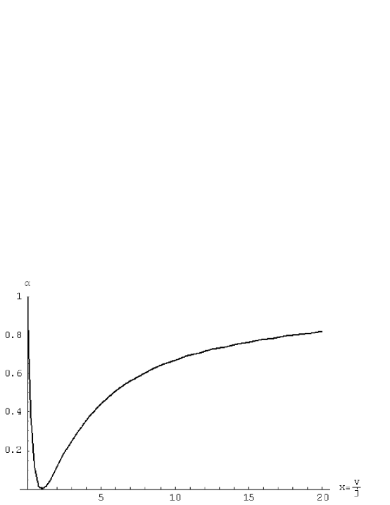
Figure 2: (Color Online) Plot of $\alpha$ Vs. the ratio of the impurity coulomb scattering potential and the exchange coupling to the impurity.

Appendix A Perturbation Expansion to second order

We begin with a Hamiltonian which characterizes the ground state wavefunctions of the the total wavefunction $\Psi\rangle$ of the system . The Hamiltonian eigenvalue problem is written as follows :

$$H|\Psi\rangle=E|\Psi\rangle$$ (125)

where $|\Psi\rangle$ is now written as an expansion of the ground states kets, which is linear superposition of orthogonal functions $|n^{(0)}\rangle$, $|k^{(1)}\rangle$, $|m^{(2)}\rangle$,… as follows

$$(H_{0}+V)(|n^{0}\rangle\lambda|k^{1}\rangle+\lambda^{2}|m^{2}\rangle+...)=(E^{(0)}+\lambda E^{(2)}+E^{(2)}\lambda^{2}+....)(|n^{0}\rangle\lambda|k^{1}\rangle+\lambda^{2}|m^{2}\rangle+...)$$ (126)

where the superindex ⁿ refers to the order of the expansion. Since they are coefficients of an order-n polynomial, they are linearly independent.

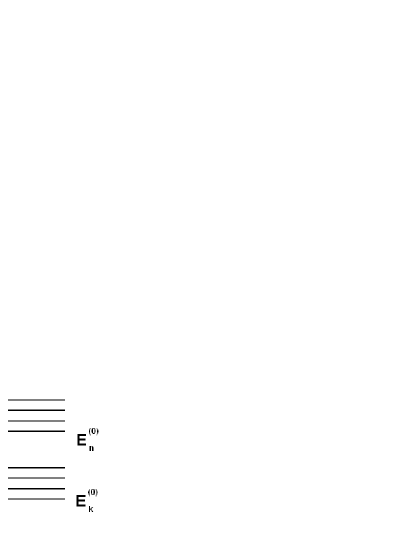
Figure 3: (Color Online) Spectrum of energy levels in a degenerate system.

Taking the O(1) equation from 126 above, we have :

$$O(1):H_{0}|n^{0}\rangle=E_{0}|n^{0}\rangle$$ (127)

$$\Rightarrow$$ (128)

$$\langle n^{0}|H_{0}|n^{0}\rangle=E_{0}\langle n^{0}|n^{0}\rangle$$ (129)

$$O(\lambda):\lambda H_{0}|k^{1}\rangle+\lambda V|n^{0}\rangle=\lambda E_{0}|k^{1}\rangle+\lambda E^{1}|n^{0}\rangle$$ (130)

$$O(\lambda^{2}):\lambda^{2}H_{0}|m^{2}\rangle+\lambda^{2}V|k^{1}\rangle=\lambda^{2}E_{1}|k^{1}\rangle+\lambda^{2}E^{2}|n^{0}\rangle$$ (131)

We now arrive at the expansion coefficients for the first order correction to the wavefunctions , by multiplying the O($\lambda$) equation above by the $\langle n^{0}|$ ket and we arrive at the following equation :

$$\lambda\langle n^{0}|H_{0}|k^{1}\rangle+\lambda\langle n^{0}|V|n^{0}\rangle=\lambda E^{(0)}_{n}\langle n^{(0)}|k^{(1)}\rangle+\lambda E^{(1)}\langle n^{(0)}|n^{(0)}\rangle$$ (133)

$\vee$ n $\neq$ k, we have :

$$\langle n^{(0)}|V|n^{(0)}\rangle=E^{(1)},$$ (134)

which is the first-order correction to the total energy. Taking the O($\lambda$) equation, we multiply across by the ket $|k^{(0)}\rangle$ armed with the decomposition of $|k^{(1)}\rangle$ onto the vector space $|k^{(0)}\rangle$, which we can write as $|k^{(1)}\rangle$ = $\sum_{k}C_{kn}$ $|k^{(0)}\rangle$. This can be written more succinctly in the outer product notation $|k^{(1)}\rangle$ = $|k^{(1)}\rangle\langle n^{(0)}|n^{(0)}\rangle$. We now write the O($\lambda$) equation as :

$$\lambda\langle|k^{(0)}|H_{0}\|k^{(1)}\rangle+\lambda\langle|k^{(0)}|V|n^{(0)}\rangle=\lambda E^{(0)}_{n}\langle k^{(0)}|k^{(1)}\rangle+\lambda E^{(1)}\langle k^{(0)}|n^{(0)}\rangle.$$ (135)

Now, $\vee$ n $\neq$ k, we seek the coefficients of the expansion of the first order wavefunction in ground state kets, as follows :

$$\displaystyle\sum_{n\neq k}\langle k^{(0)}|H_{0}C_{k}|k^{(0)}\rangle+\langle k^{(0)}|V|n^{(0)}\rangle=E^{(0)}_{n}\langle k^{(0)}C_{k}|k^{(0)}\rangle+E^{(1)}\langle k^{(0)}|n^{(0)}\rangle$$ (136)

$$\Rightarrow$$ (137)

$$C_{k}^{(1)}=\displaystyle\sum_{n\neq k}\frac{|V_{kn}|}{E^{0}_{n}-E^{(0)}_{k}}$$ (138)

In order to find the second order perturbation expansion coefficients, we iterative this progress further by using the O ($\lambda^{2}$), which has the following form :

$$H_{0}|m^{(2)}\rangle+V|k^{(1)}\rangle=E^{(0)}|m^{(2)}\rangle+E^{(1)}|k^{(1)}\rangle+E^{(2)}|n^{(0)}\rangle$$ (139)

$$H_{0}C_{m}|m^{(0)}\rangle+VC_{k}|k^{(0)}\rangle=E^{(0)}C_{m}|m^{(0)}\rangle+E^{(1)}C_{k}|k^{(0)}\rangle+E_{n}^{(2)}|n^{(0)}\rangle$$ (140)

$$(E^{(0)}_{m}-E^{(0)}_{n})C_{m}|m^{(0)}=VC_{k}|k^{(0)}+E^{(1)}_{k}C_{k}|k^{(0)}\rangle+E^{(2)}_{m}|n^{(0)}\rangle$$ (141)

Next, we multiply across by the ket $|m^{0}\rangle$ and make use of the fact that the each basis $|n^{0}\rangle$, $|k^{0}\rangle$,$|m^{0}\rangle$ are all orthonormal sets, as follows :

$$C_{m}(E^{(0)}_{m}-E^{(0)}_{n})=V_{mk}C_{k}+E^{(1)}_{k}C_{k}\delta_{mk}+E^{(2)}_{m}\delta_{mn}$$ (142)

Next we take the case, whereby n$\neq$k$\neq$m, which gives :

$$C_{m}=\displaystyle\sum_{m\neq n}\frac{V_{mk}C_{k}}{E^{(0)}_{m}-E^{(0)}_{n}}=\displaystyle\sum_{m\neq n}\displaystyle\sum_{n\neq k}\frac{V_{mk}V_{kn}}{(E^{(0)}_{m}-E^{(0)}_{n})(E^{(0)}_{n}-E^{(0)}_{k})}.$$ (143)

In the above equation, we have substituted in the result for the first order expansion coefficients C_k. The second order corrections to the total wavefunction are now know in terms of the matrix elements of the perturbing potential V and the ground state eigenenergies. To find the second order corrections to the energy $E^{(2)}_{n}$, take n=m$\neq$k in the above equation, which gives :

$$E^{(2)}_{n}=-V_{mm}C_{k}$$ (144)

Figure 4: (Color Online) Exchange split ferromagnetic ground state.