Strongly correlated electron systems; heavy fermionsMagnetoresistance Quantum phase transitions

Magnetoresistance of the heavy-fermion metal CeCoIn_5

Abstract

The magnetoresistance (MR) of CeCoIn_5 is notably different from that expected for orbital MR due to the Lorentz force and described by Kohler’s rule which holds in many conventional metals. We show that a pronounced crossover from negative to positive MR of CeCoIn_5 that occurs at elevated temperatures is determined by the dependence of the effective mass $M^{*}(B,T)$ on both magnetic field $B$ and temperature $T$. Thus, the crossover is regulated by the universal behavior of $M^{*}(B,T)$ observed in heavy-fermion metals. This behavior is exhibited by $M^{*}(B,T)$ when a strongly correlated electron system transits from the Landau Fermi liquid behavior induced by the application of magnetic field to the non-Fermi liquid behavior taking place at rising temperatures. Our calculations of MR are in good agreement with facts and reveal new scaling behavior of MR.

An explanation of the rich and striking behavior of strongly correlated electron system in heavy fermion (HF) metals is, as years before, among the main problems of the condensed matter physics. One of the most interesting and puzzling issues in the research of HF metals is the anomalous normal-state transport properties. HF metals show a number of distinctive transport properties, among which is the magnetoresistance (MR) of HF metals. Measurements of MR on CeCoIn_5 [1, 2] have shown that this is notably different from that expected for weak-field orbital MR and described by Kohler’s rule which holds in many conventional metals, see e.g. [3]. MR of CeCoIn_5 exhibits a crossover from negative to positive MR that occurs in fixed magnetic fields $B$ with increasing temperature $T$, so that at the high fields and relatively low temperatures MR becomes negative [1, 2].

This crossover is hard to explain within the conventional Fermi liquid theory for metals and in terms of Kondo systems [4] and therefore it is assumed that the crossover can be attributed to some energy scales causing a change in character of spin fluctuations with increasing the applied magnetic field strength [1]. It is widely believed that such quantum fluctuations becoming sufficiently strong suppress quasiparticles at a quantum phase transition and when the system in question transits from its Landau-Fermi liquid (LFL) regime to non-Fermi liquid (NFL) behavior [5, 6, 7].

On the other hand, even early measurements carried out on HF metals gave evidences in favor of the existence of quasiparticles. For example, the application of magnetic field $B$ restores LFL regime of HF metals which in the absence of the field demonstrates NFL behavior. In that case the empirical Kadowaki-Woods ratio $K$ is conserved, $K=A(B)/\gamma_{0}^{2}(B)\propto A(B)/\chi^{2}(B)=const$ [8, 9] where $C/T=\gamma_{0}$, $C$ is the heat capacity, $\chi$ is magnetic susceptibility and $A(B)$ is the coefficient determining the temperature dependence of the resistivity $\rho=\rho_{0}+A(B)T^{2}$. Here $\rho_{0}$ is the residual resistance. The observed conservation of $K$ can be hardly accounted for within scenarios when quasiparticles are suppressed, for there is no reason to expect that $\gamma_{0}(B)$, $\chi(T)$, $A(B)$ and other transport and thermodynamic quantities like the thermal expansion coefficient $\alpha(B)$ are affected by the fluctuations or localization in a correlated fashion.

Quasiparticles were observed in LFL regime in measurements of transport properties on CeCoIn_5 [10]. While it is extensively accepted that the NFL behavior is determined by the critical fluctuations, Kondo lattice [5, 6, 7] and multiple energy scales [11], therefore in that scenario the crossover region has to be formed by the fluctuations and scales rather then by quasiparticles. Analyzing thermodynamic quantities, it was shown that quasiparticles exist in both the LFL and the crossover regimes when strongly correlated Fermi systems such as HF metals [12, 13, 14, 15, 16] or two-dimensional ^3He [17] transit from its LFL to NFL behavior. Therefore it is of crucial importance to verify whether quasiparticles characterized by their effective mass $M^{*}$ still exist and determine the transport properties of HF metals in the crossover region. As we will see, measurements of MR in the crossover region can present indicative data on the availability of quasiparticles. Fortunately, such measurements of MR were carried out on CeCoIn_5 when the system transit from the LFL to NFL behavior at elevated temperatures and fixed magnetic fields [1, 2].

In this Letter we analyze MR of CeCoIn_5 and show that the crossover from negative to positive MR that occurs at elevated temperatures and fixed magnetic fields can be well captured utilizing fermion condensation quantum phase transition (FCQPT) based on the quasiparticles paradigm [18, 14, 19, 20]. We demonstrate that crossover is regulated by the universal behavior of the effective mass $M^{*}(B,T)$ observed in many heavy-fermion metals and is exhibited by $M^{*}(B,T)$ when HF metal transits from the LFL behavior induced by the application of magnetic field to NFL behavior taking place at rising temperatures. Our calculations of MR are in good agreement with facts and allow us to reveal new scaling behavior of MR. Thus, we show that the transport properties are mainly determined by quasiparticles rather then by the critical fluctuations, Kondo lattice and energy scales which are expected to arrange the behavior in the transition region.

To study universal low temperature features of HF metals, we use the model of homogeneous heavy-fermion liquid with the effective mass $M^{*}(T,B,x)$, where the number density $x=p_{F}^{3}/3\pi^{2}$ and $p_{F}$ is the Fermi momentum [21]. This permits to avoid complications associated with the crystalline anisotropy of solids [15]. We first outline the case when at $T\to 0$ the heavy-electron liquid behaves as LFL and is brought to the LFL side of FCQPT by tuning a control parameter like $x$. At elevated temperatures the system transits to the NFL state. The dependence $M^{*}(T,x)$ is governed by Landau equation [21]

$$\frac{1}{M^{*}(T,x)}=\frac{1}{M}+\int\frac{{\bf p}_{F}{\bf p}}{p_{F}^{3}}F({\bf p_{F}},{\bf p})\frac{\partial n({\bf p},T,x)}{\partial{p}}\frac{d{\bf p}}{(2\pi)^{3}},$$ (1)

where $n({\bf p},T,x)$ is the distribution function of quasiparticles and $F({\bf p}_{F},{\bf p})$ Landau interaction amplitude. At $T=0$, eq. (1) reads [21] $M^{*}/M=1/(1-N_{0}F^{1}(p_{F},p_{F})/3)$. Here $N_{0}$ is the density of states of a free electron gas, $F^{1}(p_{F},p_{F})$ is the $p$-wave component of Landau interaction amplitude $F$. Taking into account that $x=p_{F}^{3}/3\pi^{2}$, we rewrite the amplitude as $F^{1}(p_{F},p_{F})=F^{1}(x)$. When at some critical point $x=x_{FC}$, $F^{1}(x)$ achieves certain threshold value, the denominator tends to zero and the system undergoes FCQPT related to divergency of the effective mass [18, 20, 14]

$$\frac{M^{*}(x)}{M}=A+\frac{B}{x_{FC}-x},$$ (2)

where $M$ is the bare mass, eq. (2) is valid in both 3D and 2D cases, while the values of factors $A$ and $B$ depend on the dimensionality. The approximate solution of eq. (1) is of the form [16]

$$\frac{M}{{M^{*}(T)}} = \frac{M}{{M^{*}(x)}}+\beta f(0)\ln\left\{{1+\exp(-1/\beta)}\right\}$$ (3)

$$+ \lambda_{1}\beta^{2}+\lambda_{2}\beta^{4}+...,$$

where $\lambda_{1}>0$ and $\lambda_{2}<0$ are constants of order unity, $\beta=TM^{*}(T)/p_{F}^{2}$ and $f(0)\sim F^{1}(x_{FC})$. It follows from eq. (3) that the effective mass $M^{*}$ as a function of $T$ and $x$ reveals three different regimes at growing temperature. At the lowest temperatures we have LFL regime with $M^{*}(T,x)\simeq M^{*}(x)+aT^{2}$ with $a<0$ since $\lambda_{1}>0$. The effective mass as a function of $T$ decays down to a minimum and after grows, reaching its maximum $M^{*}_{M}$ at some temperature $T_{M}(x)$ then subsequently diminishing as $T^{-2/3}$ [12, 14]. Moreover, the closer is the number density $x$ to its threshold value $x_{FC}$, the higher is the rate of the growth. The peak value $M^{*}_{M}$ grows also, but the maximum temperature $T_{M}$ lowers. Near this temperature the last ”traces” of LFL regime disappear, manifesting themselves in the divergence of above low-temperature series and substantial growth of $M^{*}(x)$. Numerical calculations based on eqs. (1) and (3) show that at rising temperatures $T>T_{1/2}$ the linear term $\propto\beta$ gives the main contribution and leads to new regime when eq. (3) reads $M/M^{*}(T)\propto\beta$ yielding

$$M^{*}(T)\propto T^{-1/2}.$$ (4)

We remark that eq. (4) ensures that at $T\geq T_{1/2}$ the resistivity behaves as $\rho(T)\propto T$ [14].

Figure 1: Schematic plot of the normalized effective mass $M^{*}_{N}=M^{*}(T/T_{M})/M^{*}_{M}$ ($M^{*}_{M}$ is its maximal value at $T=T_{M}$) versus the normalized temperature $T_{N}=T/T_{M}$. Several regions are shown. First goes the LFL regime ($M^{*}_{N}(T_{N})\sim$ const) at $T_{N}\ll 1$, then the transition regime (the hatched area) where $M^{*}_{N}$ reaches its maximum. At elevated temperatures $T^{-2/3}$ regime occurs followed by $T^{-1/2}$ behavior, see eq. (4).

Near the critical point $x_{FC}$, with $M/M^{*}(x\to x_{FC})\to 0$, the behavior of the effective mass changes dramatically because the first term on the right-hand side of eq. (3) vanishes, the second term becomes dominant, and the effective mass is determined by the homogeneous version of (3) as a function of $T$. As a result, the scale $M/M^{*}$ vanishes and we get to scale $M^{*}$ in $M^{*}_{M}$ and $T$ in $T_{M}$. These scales can be viewed as natural ones. The schematic plot of the normalized effective mass $M^{*}_{N}=M^{*}/M^{*}_{M}$ versus normalized temperature $T_{N}=T/T_{M}$ is reported fig. 1. In fig. 1 both $T^{-2/3}$ and $T^{-1/2}$ regimes are marked as NFL ones since the effective mass depends strongly on temperature. The temperature region $T\simeq T_{M}(x)$ signifies the crossover between the LFL regime with almost constant effective mass and NFL behavior, given by $T^{-2/3}$ dependence. Thus temperatures $T\sim T_{M}$ can be regarded as the crossover between LFL and NFL regimes. It turns out that $M^{*}(T,x)$ in the entire $T\leq T^{-1/2}$ range can be well approximated by a simple universal interpolating function [14, 16, 12]. The interpolation occurs between the LFL ($M^{*}\propto T^{2}$) and NFL ($M^{*}\propto T^{-1/2}$, see eq. (4)) regimes thus describing the above crossover. Introducing the dimensionless variable $y=T_{N}=T/T_{M}$, we obtain the desired expression

$$\frac{M^{*}(T/T_{N},x)}{M^{*}_{M}}={M^{*}_{N}(y)}\approx\frac{M^{*}(x)}{M^{*}_{M}}\frac{1+c_{1}y^{2}}{1+c_{2}y^{8/3}}.$$ (5)

Here $M^{*}_{N}(y)$ is the normalized effective mass, $c_{1}$ and $c_{2}$ are parameters, obtained from the condition of best fit to experiment. To correct the behavior of $M^{*}_{N}(y)$ at rising temperatures we add a term to eq. (5) and obtain

$$M^{*}_{N}(y)\approx\frac{M^{*}(x)}{M^{*}_{M}}\left[\frac{1+c_{1}y^{2}}{1+c_{2}y^{8/3}}+c_{3}\frac{\exp(-1/y)}{\sqrt{y}}\right],$$ (6)

where $c_{3}$ is a parameter. The last term on the right hand side of eq. (6) makes $M^{*}_{N}$ satisfy eq. (4) at rising temperatures $T/T_{M}>2$.

At small magnetic fields $B$ (that means that the Zeeman splitting is small), the effective mass does not depend on spin variable and $B$ enters eq. (1) as $B\mu_{B}/T$ making $T_{M}\propto B\mu_{B}$ where $\mu_{B}$ is the Bohr magneton [14, 16]. The application of magnetic field restores the LFL behavior, and at $T=0$ the effective mass depends on $B$ as [12, 14]

$$M^{*}(B)\propto(B-B_{c0})^{-2/3},$$ (7)

where $B_{c0}$ is the critical magnetic field driving both HF metal to its magnetic field tuned QCP and corresponding Néel temperature toward $T=0$. In some cases $B_{c0}=0$. For example, the HF metal CeRu_2Si_2 is characterized by $B_{c0}=0$ and shows neither evidence of the magnetic ordering or superconductivity nor the LFL behavior down to the lowest temperatures [22]. In our simple model $B_{c0}$ is taken as a parameter. We conclude that under the application of magnetic filed the variable

$$y=T/T_{M}\propto\frac{T}{\mu_{B}(B-B_{c0})}$$ (8)

remains the same and the normalized effective mass is again governed by eqs. (5) and (6) which are the final result of our analytical calculations. We note that the obtained results are in agreement with numerical calculations [14, 12].

The normalized effective mass $M^{*}_{N}(y)$ can be extracted from experiments on HF metals. For example, $M^{*}(T,B)\propto C(T)/T\propto S(T)/T\propto\chi_{AC}(T)$, where $S(T)$ is the entropy, $C(T)$ is the specific heat and $\chi_{AC}(T)$ is ac magnetic susceptibility. If the corresponding measurements are carried out at fixed magnetic field $B$ (or at fixed both the concentration $x$ and $B$) then, as it seen from fig. 1, the effective mass reaches the maximum at some temperature $T_{M}$. Upon normalizing both the effective mass by its peak value $M^{*}_{M}$ at each field $B$ and the temperature by $T_{M}$, we observe that all the curves have to merge into single one, given by eqs. (5) and (6) thus demonstrating a scaling behavior.

To verify eq. (4), we use measurements of $\chi_{AC}(T)$ in CeRu_2Si_2 at magnetic field $B=0.02$ mT at which this HF metal demonstrates the NFL behavior [22]. It is seen from fig. 2 that eq. (4) gives good description of the facts in the extremely wide range of temperatures. The inset of fig. 2 exhibits a fit for $M^{*}_{N}(y)$ extracted from measurements of $\chi_{AC}(T)$ at different magnetic fields, clearly indicating that the function given by eq. (5) represents a good approximation for $M^{*}_{N}(y)$.

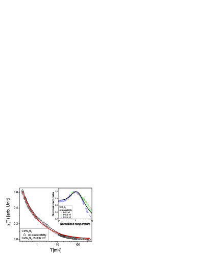
Figure 2: Temperature dependence of the $ac$ susceptibility $\chi_{AC}$ for CeRu_2Si_2. The solid curve is a fit for the data shown by the triangles at $B=0.02$ mT and represented by the function $\chi(T)=a/\sqrt{T}$ given by eq. (4) with $a$ being a fitting parameter. Inset shows the normalized effective mass versus normalized temperature $y$ extracted from $\chi_{AC}$ measured at different fields as indicated in the inset [22]. The solid curve traces the universal behavior of $M^{*}_{N}(y)$ determined by eq. (5). Parameters $c_{1}$ and $c_{2}$ are adjusted to fit the average behavior of the normalized effective mass $M^{*}_{N}(y)$.

$M^{*}_{N}(y)$ extracted from the entropy $S(T)/T$ and magnetization $M$ measurements on the ³He film [23] at different densities $x<x_{FC}$ is reported in the left panel of fig. 3. In the same panel, the data extracted from the heat capacity of the ferromagnet CePd_0.2Rh_0.8 [24] and the AC magnetic susceptibility of the paramagnet CeRu_2Si_2 [22] are plotted for different magnetic fields. It is seen that the universal behavior of the normalized effective mass given by eq. (5) and shown by the solid curve is in accord with the experimental facts. All 2D ^3He substances are located at $x<x_{FC}$, where the system progressively disrupts its LFL behavior at elevated temperatures. In that case the control parameter, driving the system towards its critical point $x_{FC}$ is merely the number density $x$. It is seen that the behavior of $M^{*}_{N}(y)$, extracted from $S(T)/T$ and magnetization $M$ of 2D ^3He looks very much like that of 3D HF compounds. In the right panel of fig. 3, the normalized data on $C(y)$, $S(y)$, $y\chi(y)$ and $M(y)+y\chi(y)$ extracted from data collected on CePd_1-xRh_x [24] , ^3He [23], CeRu_2Si_2 [22], and YbRu_2Si_2 [11] respectively are presented. Note that in the case of YbRu_2Si_2, the variable $y=B\mu_{B}/T_{M}$. As seen from eq. (5), this representation of the variable $y$ is correct, and $B\mu_{B}$ makes sense of the variable, while the temperature is a fixed parameter. All the data show a kink at $y\geq 1$ taking place as soon as the system enters the transition region from the LFL state to the NFL one. Again, we conclude that the presence of the kink is mainly determined by the behavior of the effective mass at the transition region rather then by the critical fluctuations or Kondo scales [11].

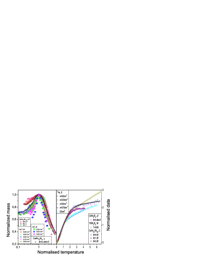
Figure 3: The left panel. The normalized effective mass $M^{*}_{N}$ versus the normalized temperature $y=T/T_{M}$. The behavior of $M^{*}_{N}$ is extracted from measurements of $S(T)/T$ and magnetization $M$ on 2D ^3He [23]), from $ac$ susceptibility $\chi_{AC}(T)$ collected on CeRu_2Si_2 [22] and from $C(T)/T$ collected on CePd_1-xRh_x [24]. The data are collected at different densities and magnetic fields as shown in the left bottom corner. The solid curve traces the universal behavior of the normalized effective mass determined by eq. (5). Parameters $c_{1}$ and $c_{2}$ are adjusted for $\chi_{N}(T_{N},B)$ at $B=0.94$ mT. The right panel. The normalized specific heat $C(y)$ of CePd_1-xRh_x at different magnetic fields $B$, normalized entropy $S(y)$ of ^3He at different number densities $x$, and the normalized $y\chi(y)$ at $B=0.94$ mT versus normalized temperature $y$ are shown. The upright triangles depict the normalized ‘average’ magnetization $M+B\chi$ collected on YbRu_2Si_2 [11]. The kink in all the data is clearly seen in the transition region $y\geq 1$. The solid curve represents $yM^{*}_{N}(y)$ with parameters $c_{1}$ and $c_{2}$ adjusted for magnetic susceptibility of CeRu_2Si_2 at $B=0.94$ mT.

By definition, MR is given by

$$\rho_{mr}(B,T)=\frac{\rho(B,T)-\rho(0,T)}{\rho(0,T)},$$ (9)

We apply eq. (9) to study MR of strongly correlated electron liquid versus temperature $T$ as a function of magnetic field $B$. The resistivity $\rho(B,T)$ is

$$\rho(B,T)=\rho_{0}+\Delta\rho(B,T)+\Delta\rho_{L}(B,T),$$ (10)

where $\Delta\rho(B,T)=c(M^{*}(B,T))^{2}T^{2}$, and $c$ is a constant, and the classical contribution $\Delta\rho_{L}(T,B)$ to MR due to orbital motion of carriers induced by the Lorentz force obeys the Kohler’s rule [3]:

$$\frac{\Delta\rho_{L}(B,T)}{\rho(0,T)}\simeq F\left(\frac{\mu_{B}B}{\rho(0,T)}\right).$$ (11)

Function $F$ is determined by the details of metal. We note that $\Delta\rho_{L}(B)$ $\ll\rho(0,T)$ as it is assumed in the weak-field approximation. Suppose that the temperature is not very low, so that $\rho_{0}\leq\Delta\rho(B=0,T)$, and $B\geq B_{c0}$. Substituting (10) in (9), we find that

$$\rho_{mr}(B,T)\simeq\frac{\Delta\rho_{L}(B,T)}{\rho(0,T)}$$ (12)

$$+ cT^{2}\frac{(M^{*}(B,T))^{2}-(M^{*}(0,T))^{2}}{\rho(0,T)}.$$

Consider the qualitative behavior of MR described by eq. (12) as a function of $B$ at a certain temperature $T=T_{0}$. In weak magnetic fields, when $T_{0}\geq T_{1/2}$ and the system exhibits NFL regime (see fig. 1), the main contribution to MR is made by the term $\Delta\rho_{L}(B)$, because the effective mass is independent of the applied magnetic field. Hence, $|M^{*}(B,T)-M^{*}(0,T)|/M^{*}(0,T)\ll 1$ and the leading contribution is made by $\Delta\rho_{L}(B)$. As a result, MR is an increasing function of $B$. When $B$ becomes so high that $T_{M}(B)\sim\mu_{B}B\sim T_{0}$, the difference $(M^{*}(B,T)-M^{*}(0,T))$ becomes negative and MR as a function of $B$ reaches its maximum value at $T_{M}(B)\sim T_{0}$. As $B$ increases still further, when $T_{M}(B)>T_{0}$, the effective mass $M^{*}(B,T)$ becomes a decreasing function of the magnetic field, as follows from eq. (7). As $B$ increases,

$$\frac{(M^{*}(B,T)-M^{*}(0,T))}{M^{*}(0,T)}\to-1,$$ (13)

and the magnetoresistance, being a decreasing function of $B$, is negative.

Now study the behavior of MR as a function of $T$ at a certain value $B_{0}$ of magnetic field. At low temperatures $T\ll T_{M}(B_{0})$, it follows from eqs. (5) and (7) that

$$\frac{M^{*}(B_{0})}{M^{*}(T)}\ll 1,$$ (14)

and it follows from eq. (13) that $\rho_{mr}(B_{0},T)\sim-1$, because $\Delta\rho_{L}(B)/\rho(0,T)\ll 1$. We note that $B_{0}$ must be relatively high to guarantee that $M^{*}(B_{0})/M^{*}(T)$ $\ll 1$. As the temperature increases, MR increases, remaining negative. At $T\simeq T_{M}(B_{0})$, MR is approximately zero, because $M^{*}(B_{0})\simeq M^{*}(T)$ and $\rho(B_{0},T)\simeq\rho(0,T)$ at this point. This allows us to conclude that the change of the temperature dependence of resistivity $\rho(B_{0},T)$ from quadratic to linear manifests itself in the transition from negative MR to positive. One can also say that the transition takes place when the system transits from the LFL behavior to the NFL one. At $T\geq T_{M}(B_{0})$, the leading contribution to MR is made by $\Delta\rho_{L}(B_{0})$ and MR reaches its maximum. At $T_{M}(B_{0})\ll T$, MR is a decreasing function of the temperature, because

$$\frac{|M^{*}(B,T)-M^{*}(0,T)|}{M^{*}(0,T)}\ll 1,$$ (15)

and $\rho_{mr}(B_{0},T)\ll 1$.

The both transitions [25] (from positive MR to negative MR with increasing $B$ at a fixed temperature $T$ and from negative MR to positive MR with increasing $T$ at a fixed value of $B$) have been detected in measurements of the resistivity of CeCoIn_5 in a magnetic field [1].

Let us turn to quantitative analysis of MR. As it was mentioned above, we can safely assume that the classical contribution $\Delta\rho_{L}(B,T)$ to MR is small as compared with $\Delta\rho(B,T)$. This fact allows us to make our analysis and results transparent and simple since the behavior of $\Delta\rho_{L}(B_{0})$ is not known in the case of HF metals. Consider the ratio $R^{\rho}=\rho(B,T)/\rho(0,T)$ and assume for a while that the residual resistance $\rho_{0}$ is small in comparison with the temperature dependent terms. Taking into account eq. (10) and that $\rho(0,T)\propto T$, we obtain from eq. (12) that

$$R^{\rho}=\rho_{mr}+1=\frac{\rho(B,T)}{\rho(0,T)}\propto T(M^{*}(B,T))^{2}.$$ (16)

It follows from eqs. (5) and (16) that the ratio $R^{\rho}$ reaches its maximum value $R^{\rho}_{M}$ at some temperature $T_{\rm Rm}\sim T_{M}$. If the ratio is measured in terms of its maximum value $R^{\rho}_{M}$ and $T$ is measured in terms of $T_{\rm Rm}\sim T_{M}$ then it is seen from eqs. (5), (6) and (16) that the normalized ratio

$$R^{\rho}_{N}(y)=\frac{R^{\rho}(B,T)}{R^{\rho}_{M}(B)}\simeq y(M^{*}_{N}(y))^{2}$$ (17)

becomes a universal function of the only variable $y=T/T_{\rm Rm}$. To verify eq. (17), we use MR obtained in measurements on CeCoIn₅, see fig. 1(b) of Ref. [1]. The results of the normalization procedure of MR are reported in fig. 4. It is clearly seen that the data collapse into the same curve, indicating that MR well obeys the scaling behavior given by eq. (17). This scaling behavior obtained directly from the experimental facts is a vivid proof that MR is predominantly governed by the effective mass $M^{*}(B,T)$.

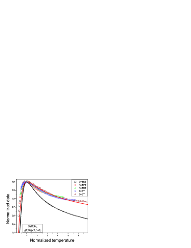
Figure 4: The normalized ratio $R^{\rho}_{N}(y)$ given by eq. (17) versus normalized temperature $y=T/T_{\rm Rm}$. The normalized ratio were extracted from MR shown in fig. 6 and collected on CeCoIn_5 at fixed magnetic fields $B$ [1] listed in the right upper corner. The starred line represents our calculations based on eqs. (5) and (17) with the parameters extracted from $ac$ susceptibility of $\rm CeRu_{2}Si_{2}$ (see the caption to fig. 2). The solid line displays our calculations based on eqs. (6) and (17); only one parameter was used to fit the data, while the other were extracted from the $ac$ susceptibility measured on CeRu_2Si_2.

Now we are in position to calculate $R^{\rho}_{N}(y)$ given by eq. (17). Using eq. (5) to parametrize $M^{*}_{N}(y)$, we extract parameters $c_{1}$ and $c_{2}$ from measurements of the magnetic $ac$ susceptibility $\chi$ on $\rm CeRu_{2}Si_{2}$ [22] and apply eq. (17) to calculate the normalized ratio. It is seen that the calculations shown by the starred line in fig. 4 start to deviate from the experimental facts at elevated temperatures. To improve the description, we employ eq. (6) which describes the behavior of the effective mass at elevated temperatures in accord with eq. (4) and ensures that at these temperatures the resistance behaves as $\rho(T)\propto T$. In fig. 4, the fit of $R^{\rho}_{N}(y)$ by eq. (6) is shown by the solid line. Constant $c_{3}$ is taken as a fitting parameter, while the other were extracted from $ac$ susceptibility of CeRu_2Si_2 as described in the caption to fig. 2.

Before discussing the magnetoresistance $\rho_{mr}(B,T)$ given by eq. (9), we consider the magnetic field dependencies of both the peak value $R_{\rm max}(B)$ of MR and peak temperature $T_{\rm Rm}(B)$ at which $R_{\rm max}(B)$ takes place. It is possible to use eq. (16) which relates the position and value of the peak with the function $M^{*}(B,T)$. To do this, we have to take into account the classical contribution $\Delta\rho_{L}(B,T)$ to MR and the residual resistance $\rho_{0}$ which prevent $T_{\rm Rm}(B)$ from vanishing and makes $R_{\rm max}(B)$ finite at $B\to B_{c0}$. Therefore, MR is a continuous function at the quantum critical point $B_{c0}$ in contrast to $M^{*}(B,T)$ which peak value diverges and the peak temperature tends to zero at the point as it follows from eqs. (7) and (8). As a result, we have to substitute $B_{c}$ for $B_{c0}$ and take $B_{c}$ as a parameter. Upon modifying eq. (16) by taking into account $\Delta\rho_{L}(B,T)$ and $\rho_{0}$, we obtain

$$T_{\rm Rm}(B)\simeq b_{1}(B-B_{c}),$$ (18)

$$R_{\rm max}(B)\simeq\frac{b_{2}(B-B_{c})^{-1/3}-1}{b_{3}(B-B_{c})^{-1}+1}.$$ (19)

Here $b_{1}$, $b_{2}$, $b_{3}$ and $B_{c}$ are fitting parameters. It is pertinent to note that when deriving eq. (19), eq. (18) was employed in substituting $(B-B_{c})$ for $T$. Then, eqs. (18) and (19) are not valid at $B<B_{c0}$ when the HF metal obtains both the antiferromagnetic order and LFL behavior. In fig. 5, we show the field dependence of both $T_{\rm Rm}$ and $R_{\rm max}$, extracted from measurements of MR [1]. It is seen that both $T_{\rm Rm}$ and $R_{\rm max}$ are well described by eqs. (18) and (19) with $B_{c}=$3.8 T. We note that this value of $B_{c}$ is in good agreement with observations obtained from the $B-T$ phase diagram of CeCoIn_5, see fig. 3 of Ref. [1].

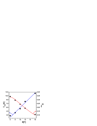
Figure 5: The peak temperatures $T_{\rm Rm}$ (squares) and the peak values $R_{\rm max}$ (triangles) versus magnetic field $B$ extracted from measurements of MR [1]. The solid lines represent our calculations based on eqs. (18) and (19).

To calculate MR $\rho_{mr}(B,T)$, we apply eqs. (17) to describe the universal behavior of MR, eq. (5) to describe the behavior of the effective mass and eqs. (18) and (19) to assign the absolute values to MR. Figure 6 shows the calculated MR versus temperature as a function of magnetic field $B$, together with the facts taken from Ref. [1]. We recall that the contributions coming from $\Delta\rho_{L}(B,T)$ and $\rho_{0}$ were omitted. As seen from fig. 6, our description of the facts is quite good and we conclude that main contribution to MR comes from the dependence of the effective mass on the applied magnetic magnetic field $B$.

Figure 6: MR versus temperature $T$ as a function of magnetic field $B$. The experimental data on MR were collected on CeCoIn_5 at fixed magnetic field $B$ [1] shown in the right bottom corner of the figure. The solid lines represent our calculations, eq. (5) is used to fit the effective mass entering eq. (17).

In summary, we have performed a study of MR of the HF metal CeCoIn_5 within the framework of the fermion condensation quantum phase transition. Obtained results are in good agreement with facts and have allowed us to reveal new scaling behavior of MR.

References

- [1] \NamePaglione J. et al. \REVIEWPhys. Rev. Lett.912003246405.
- [2] \NameMalinowski A. \REVIEWPhys. Rev. B722005184506.
- [3] \NameZiman J. M. \BookElectrons and Phonons \PublOxford University Press, Oxford \Year1960.
- [4] \NameDaybell M. D. Steyert W. A. \REVIEWPhys. Rev. Lett.181967398.
- [5] \NameVojta M. \REVIEWRep. Prog. Phys.6620032069.
- [6] \NameLöhneysen H.v. et al.\REVIEWRev. Mod. Phys. 7920071015.
- [7] \NameGegenwart P., Si Q. Steglich F. \REVIEWNature Phys. 42008186.
- [8] \NameKadowaki K. Woods S.B. \REVIEW Solid State Commun. 581986507.
- [9] \NameTsujii N., Kontani H. Yoshimura K. \REVIEWPhys. Rev. Lett. 942005057201.
- [10] \NamePaglione J. et al. \REVIEWPhys. Rev. Lett.972006106606.
- [11] \NameGegenwart P. et al. \REVIEWScience3152007969.
- [12] \NameKhodel V. A., Zverev M. V. Yakovenko V. M. \REVIEWPhys. Rev. Lett.952005236402.
- [13] \NameClark J. W., Khodel V. A. Zverev M. V. \REVIEWPhys. Rev. B712005012401.
- [14] \NameShaginyan V. R., Amusia M. Ya. Popov K. G. \REVIEW Physics-Upsekhi502007563.
- [15] \NameShaginyan V. R. et al. \REVIEWEurophys. Lett.762006898.
- [16] \NameShaginyan V. R., Popov K. G. Stephanovich V. A. \REVIEWEurophys. Lett.79200747001.
- [17] \NameShaginyan V. R. et al. \REVIEWPhys. Rev. Lett.1002008096406.
- [18] \NameKhodel V.A. Shaginyan V. R. \REVIEWJETP Lett 511990553 .
- [19] \NameAmusia M. Ya. Shaginyan V. R. \REVIEWPhys. Rev. B632001224507.
- [20] \NameVolovik G.E. \BookQuantum Phase Transitions from Topology in Momentum Space \PublLect. Notes Phys. 718, pp. 31-73, \Year2007.
- [21] \NameLifshitz E. M. Pitaevskii L. P. \BookStatistical Physics, Part 2 \PublButterworth-Heinemann, Oxford \Year1999.
- [22] \NameTakahashi D. et al. \REVIEWPhys. Rev. B672003180407(R).
- [23] \NameNeumann M., Nyéki J. Saunders J. \REVIEWScience 31720071356.
- [24] \NamePikul A.P. et al. \REVIEWJ. Phys. Condens. Matter 182006L535.
- [25] \NameShaginyan V. R. \REVIEWJETP Lett.772003178.