A comparative study of social network models: network evolution models and nodal attribute models

Abstract

This paper reviews, classifies and compares recent models for social networks that have mainly been published within the physics-oriented complex networks literature. The models fall into two categories: those in which the addition of new links is dependent on the (typically local) network structure (network evolution models, NEMs), and those in which links are generated based only on nodal attributes (nodal attribute models, NAMs). An exponential random graph model (ERGM) with structural dependencies is included for comparison. We fit models from each of these categories to two empirical acquaintance networks with respect to basic network properties. We compare higher order structures in the resulting networks with those in the data, with the aim of determining which models produce the most realistic network structure with respect to degree distributions, assortativity, clustering spectra, geodesic path distributions, and community structure (subgroups with dense internal connections). We find that the nodal attribute models successfully produce assortative networks and very clear community structure. However, they generate unrealistic clustering spectra and peaked degree distributions that do not match empirical data on large social networks. On the other hand, many of the network evolution models produce degree distributions and clustering spectra that agree more closely with data. They also generate assortative networks and community structure, although often not to the same extent as in the data. The ERGM model turns out to produce the weakest community structure.

1 Introduction

Modeling social networks serves at least two purposes. Firstly, it helps us understand how social networks form and evolve. Secondly, in studying network-dependent social processes by simulation, such as diffusion or retrieval of information, successful network models can be used to specify the structure of interaction. A large variety of models have been presented in the physics-oriented complex networks literature in recent years, to explore how local mechanisms of network formation produce global network structure. In this paper we review, classify and compare such models.

The models are classified into two main categories: those in which the addition of new links is dependent on the local network structure (network evolution models, NEMs), and those in which the probability of each link existing depends only on nodal attributes (nodal attribute models, NAMs). NEMs can be further subdivided into growing models, in which nodes and links are added until the network contains the desired number $N$ of nodes, and dynamical models, in which the steps for adding and removing ties on a fixed set of nodes are repeated until the structure of the network no longer statistically changes. For completeness, we include in our comparative study two models from the tradition of exponential random graph models (ERGMs). One of them is based solely on nodal attributes, and the other incorporates structural dependencies. All of these models produce undirected networks without multiple links or self-links, and all networks are treated as unweighted, i.e. tie strengths are not taken into account. We note that some of the models were designed with a particular property in mind, such as a high average clustering coefficient, but we will assess their ability to reproduce several of the typical features of social networks. In addition to comparing the distributions of degree and geodesic path lengths and clustering spectra, we assess the presence or absence of communities, which in the complex networks literature are typically defined as groups of nodes that are more densely connected to nodes in the same community than to nodes in other communities Fortunato and Castellano (2008).

This paper is structured as follows. In Sections 1.1 to 1.3, we define the categories of network evolution models and nodal attribute models, and briefly review exponential random graph models. Section 1.4 discusses differences between the philosophies behind NEMs and ERGMs. We fit models from each of these categories to two empirical acquaintance networks with respect to basic network statistics. The fitting procedure is discussed in Section 3 and Appendix A.2. In Section 4, we compare higher order structures in the resulting networks with those in the data. Section 5 summarizes our results.

1.1 Network evolution models (NEMs)

Let us first present a class of network models that focuses on network evolution mechanisms. These models test hypotheses that specific network evolution mechanisms lead to specific network structure. We call these network evolution models (NEMs), and define them via three properties as follows:

1. A single network realization $G$ is produced by an iterative process that always starts from an initial network configuration $G(t_{0})$ specified in the NEM. Dynamical models often begin with an empty network, and growing models start with a small seed network.

2. The specifications of the NEM include an explicitly defined set of stochastic rules by which the network structure evolves in time. These rules concern selecting a subset of nodes and links at each time step, and adding and deleting nodes and links within this subset. The rules typically correspond to abstracted mechanisms of social tie formation such as triadic closure (Granovetter, 1973), i.e. tie formation based on the tendency of two friends of an individual to become acquainted. The rules always depend on network structure and they can sometimes also incorporate nodal attributes. The rules determine the possible transitions from one network $G(t_{k-1})$ to the next $G(t_{k})$ during the iterative process that will produce one network realization $G=G(t_{end})$.

3. The NEM includes a stopping criterion:

   1. For a growing NEM, the algorithm finishes when the network has reached a predetermined size. The typical assumption is that relevant statistical properties of the network remain invariant once the network is large enough.

   2. For a dynamical NEM, the algorithm finishes when selected network statistics no longer vary.

A growing model can be motivated as a model for social networks in several contexts. For example, on social networking sites people rarely remove links, and new users keep joining the network. Similarly, in a co-authorship network Newman (2001) derived from publication records, existing links remain while new links form. We point out that the growing models do not intend to simulate the evolution of a social network ab initio. However, the mechanisms are selected to imitate the way people might join an already established social network.

The NEMs in our comparative study include only network structure based evolution rules (that may depend on topology and tie strengths), although nodal attribute based rules are also possible. Models in which link generation is based solely on (fixed) nodal attributes belong to the category of nodal attribute models (NAMs) discussed below.

1.2 Nodal attribute models (NAMs)

We adopt the term nodal attribute models (NAMs) for network models in which the probability of edge $e_{ij}$ between nodes $i$ and $j$ being present is explicitly stated as a function of the attributes of the nodes $i$ and $j$ only, and the evolutionary aspect is absent. NAMs are often based on the concept of homophily (McPherson et al., 2001), the tendency for like to interact with like, which is known to structure network ties of various types, including friendship, work, marriage, information transfer, and other forms of relationship. Such models have also been described by the term spatial models (Boguña et al., 2004; Wong et al., 2006), referring to that the fact that the attributes of each node determine its ’location’ in a social or geographical space.

1.3 Exponential random graph models (ERGMs)

Exponential random graph models (ERGMs) (Frank and Strauss, 1986; Frank, 1991; Wasserman and Pattison, 1996; Robins et al., 2007a; Snijders et al., 2006; Robins et al., 2007b), also called $p^{\ast}$ models, are used to test to what extent nodal attributes (exogenous factors) and local structural dependencies (endogenous factors) explain the observed global structure. For example, Goodreau (2007) used ERGMs to infer that much of the global structure (measured in terms of the distributions of degree, edgewise shared partners and geodesic paths) observed in a friendship network could be captured by nodal attributes and patterns of shared partners and $k$-triangles, which are relatively local structures.

Consider a random graph $\mathbf{X}$ consisting of $N$ nodes, in which a possible tie between two nodes $i$ and $j$ is represented by a random variable $X_{ij}$, and denote the set of all such graphs by $\mathcal{X}$. Using this notation, ERGMs are defined by the probability distribution of such graphs $\mathbf{X}$

$$P_{\theta,\mathcal{X}}(X=x)=\frac{\exp{\{\theta^{t}\,\mathbf{u}(x)\}}}{c(\theta,\mathcal{X})},$$ (1)

where $\theta$ is the vector of model parameters, $\mathbf{u}(x)$ is a vector of network statistics based on the network realization $x$, and the denominator $c(\theta,\mathcal{X})$ is a normalization function that ensures that the distribution sums up to one. The selected statistics $\mathbf{u}(x)$ specify a particular ERGM model. Typically, the parameters $\theta$ of an ERGM model are determined using a maximum likelihood (ML) estimate, obtained by Markov Chain Monte Carlo (MCMC) sampling (Geyer and Thompson, 1992; Snijders, 2002). MCMC sampling heuristics are also used to draw network realizations from the distribution $P_{\theta,\mathcal{X}}$. Several software packages are designed for fitting and simulating ERGMs (including pnet, SIENA, and statnet, discussed by Robins et al. (2007b)).

1.4 Differences between NEMs and ERGMs

An important difference between network evolution models and exponential random graph models is that a NEM is determined by the rules of network evolution, whereas ERGMs do not explicitly address network evolution processes. The particular update steps employed in the iterative MCMC procedure for drawing samples are not explicitly specified in ERGMs, which are defined by the probability distribution $P_{\theta,\mathcal{X}}$, although MCMC methods can also be used to model the evolution of social networks (Snijders, 1996, 2001). A class of probability models that includes network evolution is the stochastic actor-oriented models for network change proposed by Snijders (1996), which are continuous-time Markov chain models that are implemented as simulation models. Another difference is that unlike ERGMs, NEMs explicitly specify an initial configuration from which the iteration is started, as well as a stopping criterion. However, NEMs are typically not sensitive to the initial configuration.

One of the known problems with ERGMs is that the distributions of their sufficient statistics may be multimodal (Snijders, 2002). This has been of particular concern with respect to ERGMs that include statistics related to transitivity, which is a highly relevant feature in modeling social networks. The first stochastic model to express transitivity, the Markov graph (Frank and Strauss, 1986), employed a simple triangle count term that is known to cause problems of model degeneracy (Jonasson, 1999), and to lead to instability in simulation of large networks with Markov Chain Monte Carlo (MCMC) methods (Snijders, 2002; Handcock, 2003; Goodreau, 2007). This problem seems to have been largely overcome with a recently proposed term related to triangles, the geometrically weighted edgewise shared partners statistic (GWESP) (Snijders et al., 2006; Hunter et al., 2008; Robins et al., 2007b). We include in our comparison an ERGM that includes the GWESP term. It turns out that we encounter instability even with this model. In fitting this model to our data, in the optimal parameter region a very small modification of the model parameters produces a large difference in the resulting network structure. This is discussed in Section 3 and Appendix A.2.

In contrast, transitivity is easy to incorporate in NEMs. Problems of multimodality have not been observed with NEMs. Although we do not always have theoretical certainty that the network evolution rules could not lead to multimodal distributions of network statistics, in practice the models with given parameters seem to consistently produce network realizations with similar statistics.

The NEMs and ERGMs lend themselves to testing different kinds of hypotheses about networks. ERGMs can be employed to test to what extent nodal attributes and local structural correlations explain the global structure. Although both NEMs and ERGMs can easily incorporate nodal attributes, they have rarely been included in NEMs. The NEMs proposed so far have been of a fairly generic nature, whereas the ERGM approach often aims to make inferences based on specific empirical data, often including nodal attributes. On the other hand, NEMs can be employed for testing hypotheses about network evolution, which ERGMs do not explicitly address. For example, a NEM can be used to test whether a combination of tie-strength-dependent triadic closure and global connections can produce a clearly clustered structure (Kumpula et al., 2007). Although ERGMs can also be interpreted as addressing endogenous (network structure based) selection processes via structural dependencies, the mechanisms by which new ties are created based on the existing network structure are made explicit only in NEMs.

For the dynamical NEMs treated in this paper, it is easy to generate (and estimate parameters for) networks of $10\,000$ nodes or more. The growing models can easily produce networks with millions of nodes. Based on our hands-on experience using state-of-the-art ERGM software (statnet, Handcock et al. (2003, 2007)), it seems that generating a realization from a NEM might typically have much lower computational cost than drawing a sample from an ERGM with structural dependencies. In generating network realizations from an ERGM, we used as a guideline that the number of MCMC steps, corresponding to the number of proposals for changes in the link configuration, should be large enough such that the presence or absence of a link between each dyad is likely to be changed several times. With this approach, the number of MCMC steps should be proportional to the number of dyads, implying that the complexity is at least on the order of $O(N^{2})$. This is already a much larger burden than the $O(N)$ complexity of NEMs based on local operations in the neighborhood of a selected node. Our assumption of the computational demands of ERGMs is supported by the fact that networks that have thus far been studied with ERGMs have consisted typically of at most a couple of thousands of nodes (Goodreau, 2007).

Figure 1: Categories of social network models. Within the category of NEMs, we focus on models based on triadic closure and global connections (TCG). Model labels correspond to models discussed in Section 2.

2 Description of the models

Many complex networks models study the question of whether structures observed in social networks could be explained by the network-dependent interactions of nodes, without reference to intrinsic properties of nodes. Such models are based on assumptions about the local mechanisms of tie formation, such as people meeting friends of friends, and thus forming connections with their network neighbors (triadic closure (Granovetter, 1973)). An additional mechanism to produce ’global’ connections beyond the local neighborhood is typically included to account for short average geodesic path lengths (Milgram, 1967). Such connections may arise from encounters at common hobbies, places of work, etc. In models that do not consider nodal attributes, contacts between any dyads in the network are considered equally likely. These two mechanisms, triadic closure and global connections (TCG), form the basis of all the NEMs we study in this work.

Tables 1, 2 and 3 contain more detailed descriptions of the models and their parameters, with fixed parameters given in parentheses. Values of the fixed parameters were selected according to the original authors’ choices wherever possible. We label the models using author initials.

Dynamical network evolution models

We will first look at three dynamical models that combine triadic closure and global connections (TCG) for creating new links. These were proposed by Davidsen et al. (2002) (DEB), Marsili et al. (2004) (MVS), and Kumpula et al. (2007) (KOSKK). The different ways of implementing triadic closure and deletion of links in each of these models are highlighted in Fig. 2. In triadic closure mechanism T1, a node is introduced to another node by their common neighbor. In mechanism T2, new contacts are made through search via friends: A node links to a neighbor of one of its neighbors. Dynamical models in which new links are continuously added must also include a mechanism for removing links, to avoid ending up with a fully connected network. In node deletion (ND), all links of a node are deleted. This emulates a node ’leaving’ and a newcomer joining the network. In link deletion (LD), each link has a given probability of being deleted at each time step.

The DEB model is the simplest of the three, with only two parameters, network size $N$ and the probability $p$ of deleting a node. The MVS and KOSKK models both use triadic closure mechanism T2, a two-step search in the neighborhood of a node, but the KOSKK model takes interaction strength into account. In KOSKK, new links are created preferably through strong ties, and every interaction further strengthens them. This mechanism is able to produce clear community structure (Kumpula et al., 2007), confirmed by our analysis in Section 4. The three models also differ in whether a new node can remain isolated for several time steps (as in the MVS model) or will immediately link to another node (as in KOSKK), and in whether there is a limit on the number of random connections each node can make (as in DEB). Because of such differences, it is difficult to isolate the effects of the choices of T1 versus T2 and ND versus LD. Therefore, in Section 4.5 we will combine the four mechanisms using the DEB model as a basis.

Marsili et al. (2004) did not mention which value they used in the MVS model for the probability $\lambda$ of deleting a link at each time step. We fixed $\lambda=0.001$ in our simulations, giving each tie an average ’lifetime’ of $1000$ time steps. When generating network realizations, the dynamical models MVS, DEB, and KOSKK are iterated until monitored distributions appear to become stationary. Sometimes the authors do not state which particular criterion they used. For the MVS and DEB models, we determined how many iterations (the steps described in Table 1) it takes until average degree stabilizes and its distribution appears stationary. When generating networks, we used a number of iterations above this limit. For the KOSKK model, we used a number of iterations determined by the authors to be sufficient for the distributions of degree and several other network properties to appear stationary ($2.5\times 10^{4}\times N$, where $N$ is network size, resulting in $2\times 10^{8}$ and $2.8\times 10^{7}$ for fitting to our data sets of sizes $8003$ and $1133$ presented in Section 3.2.

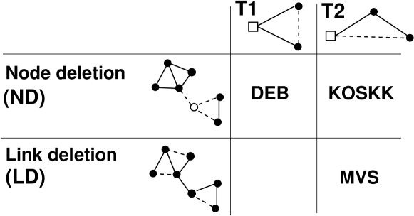
Figure 2: The dynamical network evolution models DEB, KOSKK, and MVS, classified according to the mechanisms for triadic closure and link deletion employed in them.

Table 1: Category: Dynamical network evolution models (dynamical NEMs). Three models based on triadic closure and global connections.

Parameters	Mechanisms. Number of nodes $N$ fixed; repeat steps for I) adding ties and II) deleting ties until stationary distributions are reached
DEB (Davidsen et al., 2002)
2 free $N$, $p$	I) Select a node $i$ randomly, and x a) if $i$ has fewer than two ties, introduce it to a random node x b) otherwise pick two neighbors of $i$ and introduce them if they are not already acquainted. II) Select a random node and with prob. $p$ remove all of its ties.
MVS (Marsili et al., 2004)
3 free $N$, $\xi$, $\eta$ ($\lambda\!=\!0.001$)	I) Select a node $i$ randomly, and x a) connect $i$ to another random node with probability $\eta$. x b) select a friend’s friend of $i$ (by uniformly random search) with probability $\xi$ and introduce $i$ to it if not already acquainted. II) Select a random tie and delete it with probability $\lambda$.
KOSKK (Kumpula et al., 2007)
$3$ free $N$, $p_{\Delta}$, $p_{r}$ ($w_{0}=1$, $p_{d}=0.001$, $\delta=0.5$)	I) Select a node $i$ randomly, and x a) select a friend’s friend $k$ (by weighted search) and introduce it to $i$ with prob. $p_{\Delta}$ (with initial tie strength $w_{0}$) if not already acquainted. Increase tie strengths by $\delta$ along the search path, as well as on the link $l_{ik}$ if it was already present. x b) additionally, with prob. $p_{r}$ (or with prob. $1$ if $i$ has no connections), connect $i$ to a random node $j$ (with tie strength $w_{0}$). II) Select a random node and with prob. $p_{d}$ remove all of its ties.
Nodes represent individuals and links represent ties between them. Parameters whose values were fixed according to the original authors’ choices are shown in parentheses.

Growing network evolution models

We include two growing models, proposed by Vázquez (2003) (Váz) and Toivonen et al. (2006) (TOSHK). They are described in detail in Table 2. These are to our knowledge the only growing models specifically proposed for social acquaintance networks. The motivation behind the Váz model is to produce a high level of clustering and a power law degree distribution. The TOSHK model also aims at a broad degree distribution and a high clustering coefficient, but also sets out to reproduce other features observed in social networks, such as community structure.

In TOSHK, each new node links to one or more ’initial contacts’, which in turn introduce the newcomer to some of their neighbors. In Váz, a newcomer node first links to a random node $i$, creating potential edges (Vázquez’s term) between itself and the neighbors of $i$. These ties may be realized later, generating triangles in the network. In both models, triangles are only generated between the newcomer and the neighbors of its initial contact, and further processes of introduction are ignored. As with all the models, we keep to the authors’ choices presented in the original paper. Accordingly, in the TOSHK model, we allow a newcomer to link to at most two initial contacts (see Table 2), and pick the number of secondary contacts from the uniform distribution $U[0,k]$, although this clearly limits the adaptability of the model.

Table 2: Category: Growing network evolution models (growing NEMs). Two models based on triadic closure and global connections.

Parameters	Mechanism. Repeat steps for I) adding nodes and ties II) adding ties only until network contains $N$ nodes.
TOSHK (Toivonen et al., 2006)
3 free $N$, $p$, $k$ (simplified)	I) Add a new node $i$ to the network, connecting it to one random initial contact with probability $p$, or two with probability $1-p$. II) For each random initial contact $j$, draw a number $m_{sec}$ of secondary connections from the distribution $U[0,k]$ and connect $i$ to $m_{sec}$ neighbors of $j$ if available.
Váz (Vázquez, 2003)
2 free $N$, $u$	I) With probability $1-u$, add a new node to the network, connecting it to a random node $i$. Potential edges are created between the newcomer $n$ and the neighbors $j$ of $i$ (a potential edge means that $n$ and $j$ have a common neighbor, $i$, but no direct link between them). II) With probability $u$, convert one of such potential edges generated on any previous time step to an edge. Potential edges generated by converting an edge are ignored.

Nodal attribute models

We study two nodal attribute models that differ in the dependence of link probability on distance and in the employed distance measure. These models, proposed by Boguña et al. (2004) (BPDA) and Wong et al. (2006) (WPR), are described in Table 3. The authors mention that a social space of any dimension could be used, but study the cases of 1D and 2D, respectively. We keep to their choices.

Table 3: Category: Nodal attribute models (NAMs).

Parameters	Mechanism
BPDA (Boguña et al., 2004)
3 free $N$, $\alpha$, $b$	Distribute $N$ nodes with uniform probability in a (1-dimensional) social space (a segment of length $h_{max}$). Link nodes with prob. $p=1/\left(1+\left(d/b\right)^{\alpha}\right)$, where $d$ is their distance in the social space. ($h_{max}$ can be absorbed within $b$). If treated many-dimensionally, similarity along one of the social dimensions is sufficient for the nodes to be seen as similar.
WPR (Wong et al., 2006)
4 free $N$, $H$, $p$, $p_{b}$	Distribute $N$ nodes according to a homogeneous Poisson point process in a (2-dimensional) social space of unit area. Create a link between each node pair separated by distance $d$ with probability $p+p_{b}$ if $d<H$, and with probability $p-p_{\Delta}$ if $d>H$ (where $p_{\Delta}(p,p_{b},H)$ is such that the total fraction $p$ of all possible links is generated).

ERGM with structural dependencies

As our data does not contain nodal attributes, we can only include structural terms in the exponential random graph model labeled ERGM1 (Table 4). The term edge count is an obvious choice to include, in order to match average degree. We must also include a term related to triads, considering the prevalence of transitivity social networks. We employ the geometrically weighted edgewise shared partner statistic (GWESP), proposed by Snijders et al. (2006) and formulated by Hunter et al. (2008) as

$$v(x;\tau)=e^{\tau}\sum_{i=1}^{n-2}\{1-(1-e^{\tau})^{i}\}EP_{i}(x),$$ (2)

where the edgewise shared partners statistic $EP_{i}(x)$ indicates the number of unordered pairs $\{j,k\}$ such that $x_{jk}=1$ and $j$ and $k$ have exactly $i$ common neighbors (Hunter, 2007). The simple triangle count term employed in Markov random graphs is known to cause problems of multimodality, and we are not aware of other triangle-related terms that would have been employed in ERGMs. Because we would also like to match the degree distribution to the data, we include the geometrically weighted degree term (GWD) (Snijders et al., 2006; Hunter et al., 2008)

$$u(x;\tau)=e^{\tau}\sum_{i=1}^{n-2}\{1-(1-e^{\tau})^{i}\}D_{i}(x),$$ (3)

where $D_{i}$ indicates the number of nodes with degree $i$. We fix the parameter $\tau=0.25$ as in (Goodreau, 2007). We generate network realizations using the statnet software (Handcock et al., 2007). MCMC iterations are started from an Erdős-Renyi (Bernoulli) network with average degree matching the target. We draw 5 realizations from each MCMC chain at intervals of $10^{7}$, using a burn-in of $5\times 10^{7}$ time steps. Model parameters are optimized consistently for all models with the procedure described in Section 3 and Appendix A.2.

Table 4: Category: exponential random graph models (ERGM) with structural dependencies.

Parameters	Definition
ERGM1 (Snijders et al., 2006)
4 free $N$, $\theta_{L}$, $\theta_{GWESP}$, $\theta_{GWD}$ ($\tau=0.25$)	The model is defined with three terms: edge count $L$, geometrically weighted edge-wise shared partners (GWESP) $v(x;\tau)$ (Eq. 2), and geometrically weighted degree (GWD) $u(x;\tau)$ (Eq. 3), as the probability distribution $$P_{\theta,\mathcal{X}}(X=x)=\frac{\exp{\{\theta_{L}L+\theta_{GWESP}v(x)+\theta_{GWD}u(x)\}}}{c(\theta,\mathcal{X})}$$

3 Fitting the models

In order to compare networks generated by different models, it is necessary to unify some of their properties. To this end, we fit the models to two real-world data sets with respect to as many of the most relevant network features as the model parameters allow. Our fitting method consists of simulating network realizations with different model parameters, and finding the parameter values that produce the best match to selected statistics.

3.1 Targeted features for fitting

The most important properties that we wish to align between the models and the data are the number of nodes and links. Because both of our data sets are connected components of a larger network, we focus on the properties of the largest connected component of the generated networks. Our first two fitting targets are largest connected component size $N_{LC}$ and the average number of links per node, or average degree $\bar{k}$, within the largest component. They are already sufficient for fitting the DEB and Váz models, which have only two parameters. A natural choice for the next target is some measure related to triangles, because they are highly prevalent in social networks. We will use the average clustering coefficient $\bar{c}$ (please see Appendix A.1 for the definition), which is a well-established characterization of local triangle density in the complex networks literature. All of the network evolution models in this study had as one of their aims obtaining a high clustering coefficient. These three features are sufficient for fitting the rest of the models except WPR, if we fix some of the parameters according to the original authors’ choices (please see Table 1).

If matching $N_{LC}$, $\bar{k}$ and $\bar{c}$ is not enough to fix all parameters of the model, we no longer have a straightforward choice. We considered using the assortativity coefficient and geodesic path lengths (see A.1). In the WPR model, assortativity varies closely together with the average clustering coefficient, so it could not be used as a fourth target feature. Instead, we used the average geodesic path length. We also attempted using the assortativity coefficient for fitting the KOSKK model, allowing the weight increment parameter $\delta$ to vary, but ran into a different problem: attempting high assortativity forced the weight increment parameter to zero, thereby eliminating an important feature of the weighted model and weakening the community structure. Hence, we fixed $\delta=0.5$ in accordance with the authors’ choice.

All of these measures - degree, high clustering, assortativity, and geodesic path lengths - assess important properties of social networks, which are likely to affect dynamics such as opinion formation or spreading of information (Onnela et al., 2007a; Moreno et al., 2004; Castellano et al., 2007). The average properties can typically be tuned by varying parameter values, but the general shapes of the distributions are likely to be invariable.

3.2 The friendship network at www.last.fm and the email network

We selected two social network data sets with slightly different average properties, in order to get a better picture of the adaptability of the models. They differ in average degree, average clustering coefficient, and the assortativity coefficient, although both display assortativity and high clustering.

We collected a mutual friendship network of users of the web service last.fm. At the web site www.last.fm, people can share their musical tastes and designate other users as their friends. We used for this study only the friendship information, disregarding the musical preferences. Because there are several hundred thousand users on the site worldwide, we selected users in one country, Finland, to obtain a smaller network with $8003$ individuals. The country labels were self-reported. This data set (henceforth called lastfm) represents the largest connected component of Finnish users at this site. Individuals in the resulting network have on the average $\bar{k}$ $=4.2$ friends, and a high clustering coefficient $\bar{c}$ $=0.31$. The network is highly assortative with $r=0.22$, indicating that friends of those users who have many connections at the site are themselves well connected (please see Appendix A.1 for definitions). After designating someone as a friend, there is no cost to maintaining the tie, i.e. the link never expires. This means that the data may overestimate the number of active friendships within the last-fm web site. However, the degree distribution is not broader than that observed in a network constructed from mobile phone calls (Onnela et al., 2007b), in which each contact has a real cost in time and money. Requiring ties to be reciprocated ensures that the users have at least both acknowledged one another.

We also use a smaller acquaintance network collected by Guimerà et al. (2003), based on emails between members of the University Rovira i Virgili (Tarragona). In the derived network, two individuals are connected if each sent at least one email to the other during the study period, and bulk emails sent to more than $50$ recipients are eliminated. Again, we use the largest connected component of the network. It consists of $1133$ individuals, and it is a compact network with average geodesic path length $\bar{l}$ $=3.6$, average degree $\bar{k}$ $=9.6$, fairly high average clustering coefficient $\bar{c}$ $=0.22$, and fairly small assortativity $r=0.08$.

Both of our empirical networks are unweighted, meaning that tie strengths are not specified. All of the models studied here apart from KOSKK are unweighted as well. Averaged basic statistics of both data sets are displayed in Table 6. The degree distributions, clustering spectra and degree-degree correlations of the lastfm and email networks are shown in Fig. 3, and more plots of their statistics are shown in Section 4 in connection with the fitted models.

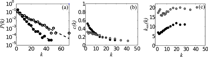
Figure 3: Properties of the lastfm data set ($\bullet$) and the email data ($\circ$). a) degree distributions, with average degrees $\bar{k}$ $=4.2$ and $9.6$, respectively.  Guimerà et al. (2003) fitted to the email data an exponential distribution $p(k)=e^{-k/k^{\ast}}$ with $k^{\ast}=9.2$, which shows as a straight line in a semilogarithmic plot. The lognormal distribution fitted the lastfm data best of the different distributions we tried (exponential, Weibull, gamma, and lognormal), although not perfectly. b) Clustering $c(k)$ decreases with degree $k$ (average clustering $\bar{c}$ $=0.31$ and $0.22$, respectively). c) Degree-degree correlations between nodes and their neighbors ($k_{nn}$ signifies average nearest neighbor degree) show that both networks are assortative (with $r=0.22$ and $r=0.08$, respectively).

Table 5 indicates which features were targeted when optimizing the parameters of each model, and displays the optimized parameters. Table 6 displays properties of the networks generated with these parameters. Due to the stochastic nature of the models, two network realizations generated with the same parameters are not likely to have exactly the same average properties. The plots and tables concerning the model networks in this paper always contain values averaged over $100$ network realizations.

Fitting to a limited number of data sets does not allow full assessment of the adaptability of the models. However, the features that we examine are similar in our two data sets as in other large scale empirical social networks, such as those based on communication via mobile phone (Onnela et al., 2007b; Seshadri et al., 2008) and Microsoft Messenger (Leskovec and Horvitz, 2008). For example, these networks have skewed degree distributions that imply the presence of high degree nodes, high average clustering coefficients $\bar{c}$, decreasing clustering spectra $c(k)$, and positive degree-degree-correlations $r$. A detailed description of the fitting procedure is included in Appendix A.2.

3.3 Adaptability of the models

Not surprisingly, for almost all models, average largest component size $\overline{N_{LC}}$ and average degrees $\bar{k}$ could be fitted closely to both data sets. For the models with only two free parameters (DEB, Váz), we had no control over other network features. These two-parameter models turn out to have excessively high average clustering coefficients for the moderate average degrees displayed in our two data sets. For most of the other models, clustering could be tuned rather closely. The TOSHK model, with its discrete parametrization of the number of triangles formed, was not able to exactly match the clustering values despite having three parameters.

For the model ERGM1, we allowed the average degree to remain slightly below the target in order to obtain correct clustering, because aiming at both correct average degree and clustering led to an instable region of model parameters. We initially attempted using automated optimization algorithms (such as snobfit (Huyer and Neumaier, 2008)) to fit the ERGM1 model, but these failed due to the instability. Based on the intuition of the model parameters obtained from the attempts at fitting, we initially selected values that roughly produced the desired $\overline{N_{LC}}$, $\bar{k}$, and $\bar{c}$, and manually modified them for a better fit. Starting from parameter values that generated networks in which the clustering coefficient matched the email data and the average degree was only slightly too small, it turned out that a very small increase in the parameter $\theta_{L}$ (done in order to increase average degree) caused average degree to jump dramatically and the clustering coefficient to plummet (see Fig. 13 in Appendix A.2). Hence, we settled for a lower value of $\bar{k}$.

Average geodesic path lengths $\bar{l}$ were approximately correct for all but the nodal attribute model treated in one dimension (BPDA), although $\bar{l}$ was used for fitting only in the WPR model. The assortativity coefficient $r$ was not used for fitting any model, although we attempted using it for fitting WPR and ERGM1. The ERGM1 model was only fitted to the email data, because generating networks of size $8000$ and fitting their parameters did not seem feasible for the ERG model.

Table 5: Targeted network features, and the fitted model parameters leading to the values closest to the lastfm and email data sets.

DEB	matched to $\overline{N_{LC}}$, $\bar{k}$
	lastfm: $N=8330,p=0.203$ email: $\,N=1138,p=0.064$
MVS	matched to $\overline{N_{LC}}$, $\bar{k}$ , $\bar{c}$
	lastfm: $N=9300,\,\xi=0.0022,\,\eta=0.000368$ email: $\,N=2270,\,\xi=0.0062,\,\eta=0.000071$
KOSKK	matched to $\overline{N_{LC}}$, $\bar{k}$ , $\bar{c}$
	lastfm: $N=8205,p_{\Delta}=0.0029,\,p_{r}=0.0008$ email: $\,N=1135,p_{\Delta}=0.0107,\,p_{r}=0.0039$
TOSHK	matched to $N$, $\bar{k}$ , $\bar{c}$
	lastfm: $N=8003,p=0.60,k=1$ email: $\,N=1133,\,p=0.06,k=3$
Váz	matched to $N$, $\bar{k}$
	lastfm: $N=8003,u=0.524$ email: $\,N=1133,\,u=0.793$
ERGM1	matched to $\overline{N_{LC}}$, $\bar{k}$ , $\bar{c}$
	lastfm: $-$ email: $N=1160,\theta_{L}=-6.962$, $\theta_{GWESP}=2.4$, $\theta_{GWD}=0.225$
BPDA	matched to $\overline{N_{LC}}$, $\bar{k}$ , $\bar{c}$
	lastfm: $N=8250,\alpha=1.915,\,b=1.51\cdot 10^{-4}$ email: $\,N=1133,\alpha=1.565,\,b=0.002032$
WPR	matched to $\overline{N_{LC}}$, $\bar{k}$ , $\bar{c}$ , $\bar{l}$
	lastfm: $N=8200,H=0.0108,p=0.000506,p_{b}=0.9994$ email: $\,N=1133,\,H=0.040,\,p=0.008498,\,p_{b}=0.991$
$\overline{N_{LC}}$: average largest component size (number of nodes), $\bar{k}$: average degree, $\bar{c}$: average clustering coefficient, $\bar{l}$: average shortest path length. $\bar{k}$, $\bar{c}$, and $\bar{l}$ were calculated for the largest component of the network.

Table 6: Basic statistics of the lastfm and email data sets and the models fitted to each.

model / data	$N_{LC}$	$L$	$\bar{k}$	$\bar{c}$	$r$	$\bar{l}$	$l_{max}$
Last-fm-fin	8003	16824	4.20	0.31	0.22	7.4	24
DEB	8009 $\pm$ 30	16858 $\pm$ 224	4.21 $\pm$ 0.05	0.38 $\pm$ 0.01	0.10 $\pm$ 0.01	7.0 $\pm$ 1.6	18.1 $\pm$ 1.4
MVS	7989 $\pm$ 38	16816 $\pm$ 153	4.21 $\pm$ 0.03	0.30 $\pm$ 0.01	0.02 $\pm$ 0.01	7.8 $\pm$ 1.6	17.4 $\pm$ 1.0
KOSKK	8006 $\pm$ 20	16849 $\pm$ 207	4.21 $\pm$ 0.05	0.31 $\pm$ 0.01	0.05 $\pm$ 0.01	7.2 $\pm$ 1.5	16.3 $\pm$ 0.9
TOSHK	8003	16791 $\pm$ 93	4.20 $\pm$ 0.02	0.34 $\pm$ 0.01	0.14 $\pm$ 0.01	6.6 $\pm$ 1.3	13.8 $\pm$ 0.6
Vàz	8003	16801 $\pm$ 171	4.20 $\pm$ 0.04	0.29 $\pm$ 0.01	0.27 $\pm$ 0.02	8.3 $\pm$ 2.6	22.6 $\pm$ 1.5
BPDA	8005 $\pm$ 31	16794 $\pm$ 141	4.20 $\pm$ 0.03	0.29 $\pm$ 0.01	0.30 $\pm$ 0.02	23.9 $\pm$ 9.3	60.1 $\pm$ 8.0
WPR	8004 $\pm$ 19	16972 $\pm$ 150	4.24 $\pm$ 0.03	0.29 $\pm$ 0.01	0.30 $\pm$ 0.02	8.1 $\pm$ 1.6	18.2 $\pm$ 1.1
model / data	$N_{LC}$	$L$	$\bar{k}$	$\bar{c}$	$r$	$\bar{l}$	$l_{max}$
Email	1133	5451	9.62	0.22	0.08	3.6	7
DEB	1133 $\pm$ 3	5452 $\pm$ 249	9.62 $\pm$ 0.43	0.45 $\pm$ 0.01	0.06 $\pm$ 0.02	3.4 $\pm$ 0.9	7.7 $\pm$ 0.7
MVS	1113 $\pm$ 1	5282 $\pm$ 77	9.48 $\pm$ 0.14	0.23 $\pm$ 0.01	0.05 $\pm$ 0.04	3.8 $\pm$ 1.1	9.6 $\pm$ 0.6
KOSKK	1134 $\pm$ 2	5425 $\pm$ 193	9.57 $\pm$ 0.34	0.22 $\pm$ 0.01	0.06 $\pm$ 0.02	3.5 $\pm$ 0.9	7.5 $\pm$ 0.6
TOSHK	1133	5453 $\pm$ 52	9.63 $\pm$ 0.09	0.29 $\pm$ 0.01	0.09 $\pm$ 0.02	3.4 $\pm$ 0.8	6.1 $\pm$ 0.3
Vàz	1133	5453 $\pm$ 136	9.63 $\pm$ 0.24	0.42 $\pm$ 0.02	0.12 $\pm$ 0.03	4.6 $\pm$ 1.7	13.6 $\pm$ 1.4
BPDA	1133 $\pm$ 1	5477 $\pm$ 172	9.67 $\pm$ 0.30	0.22 $\pm$ 0.01	0.22 $\pm$ 0.02	4.4 $\pm$ 0.8	8.4 $\pm$ 0.5
WPR	1133 $\pm$ 1	5448 $\pm$ 72	9.62 $\pm$ 0.13	0.21 $\pm$ 0.01	0.20 $\pm$ 0.03	3.6 $\pm$ 0.7	6.0 $\pm$ 0.2
ERGM1	1133 $\pm$ 8	4800 $\pm$ 460	8.47 $\pm$ 0.77	0.21 $\pm$ 0.01	0.04 $\pm$ 0.02	3.6 $\pm$ 0.84	7.5 $\pm$ 0.83
All statistics are calculated for the largest component of each network. $N_{LC}$: Largest component size, $L$: number of links, $\bar{k}$: average degree, $\bar{c}$: average clustering coefficient, $r$: assortativity coefficient, $\bar{l}$: average geodesic path length, and $l_{max}$: longest geodesic path length. The values are averaged over $100$ realizations of each network model. The standard error of the averages is displayed whenever there was fluctuation in the values.

4 Comparison of higher order statistics

Having fitted the models according to average values of particular network characteristics, we address their degree distributions $P(k)$, clustering spectra $c(k)$, and geodesic path length distributions $P(l)$. We also assess the community structure of the networks using several measures. In Section 4.5 we combine and compare the different mechanisms for triadic closure and link deletion employed in the dynamical NEMs. We use graphs to assess goodness of fit as promoted by Hunter et al. (2008).

4.1 Degree distribution

Degree distributions are shown in Fig. 4 for the email data and selected models. The exact shapes of the degree distributions produced by the models are not as important as their markedly different probabilities for the presence of high degree nodes (Fig. 4). The nodal attribute models, of which the lastfm fit of WPR is shown, produce skewed but fast-decaying degree distributions that imply the absence of nodes with very high degree. These distributions are well fit with the Poisson distribution, as shown analytically by Boguña et al. (2004) for the BPDA model. The Váz model produces a very broad degree distribution (not shown) that was shown by Vázquez (2003) to decay as power law, $P(k)\sim k^{-\gamma}$, which implies the presence of a few nodes with extremely high degree. The tails of the degree distributions produced by the dynamical NEMs and the growing TOSHK model as well as the ERGM1 model all appear to decay slower than the Poisson distribution, but faster than power law. Of these, the models TOSHK, KOSKK, and ERGM1 are displayed in Fig. 4.

In our data sets, the degree distribution decays exponentially (email) (Guimerà et al., 2003) or slower (lastfm) (Fig. 3). In larger data sets based on one-to-one communication, even broader degree distributions have been observed (Lambiotte et al., 2008; Onnela et al., 2007b; Seshadri et al., 2008). The NEMs give rise to degree distributions that match these empirical data on large acquaintance networks better than the nodal attribute models.

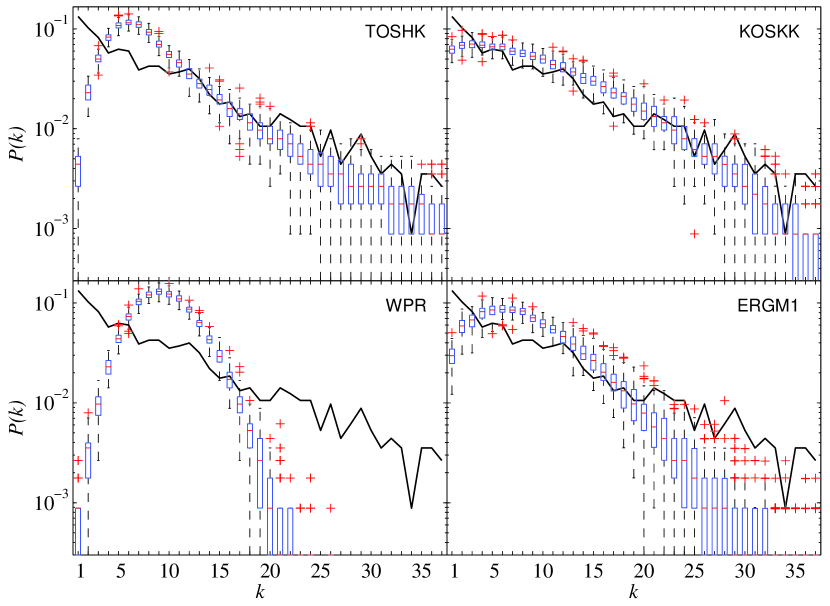
Figure 4: Degree distributions $P(k)$ of the email data (solid line) and in selected models fitted to it. The box plots display medians and first and third quartiles in $100$ network realizations. Whiskers extend from each end of the box to the most extreme values in the data within $1.5$ times the interquartile range from the ends of the box. Outliers are denoted by $+$.

4.2 Clustering spectrum

Many network models display roughly an inverse relation between node degree and clustering: $c(k)\sim\frac{1}{k}$. This holds true also for most of the NEMs studied here, of which TOSHK, KOSKK, and DEB are shown in Fig. 5, as well as for the ERGM1 model (not shown). The figures display fits to lastfm data, but results are similar for the email fits. In contrast, the homophily mechanism on which the nodal attribute models are based is seen to produce a flat clustering spectrum $c(k)=const$, shown in Fig. 5 for the lastfm fit of the WPR model. In all empirical network data that we have come across, including both of our data sets (Fig. 5) as well as acquaintance networks based on Messenger and mobile phone calls (e.g. Onnela et al. (2007b), Leskovec and Horvitz (2008)), clustering $c(k)$ decreases with increasing degree $k$ of a node. This indicates that attribute based homophily alone does not seem to explain observed network structures, supporting the findings by Masuda and Konno (2006) and Hunter et al. (2008).

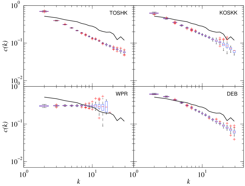
Figure 5: Clustering spectrum $c(k)$ in the lastfm data (solid line) and in models fitted to it. Averaged over $100$ network realizations.

4.3 Geodesic paths

Apart from the nodal attribute model treated one-dimensionally (BPDA), in which average geodesic path lengths are strikingly long compared to the data, all networks display reasonable path length distributions (Fig. 6). The dynamical NEMs and the TOSHK model are slightly too compact, with largest path lengths falling below those in the data. The Váz model, surprisingly, has rather long geodesic paths despite its broad degree distribution. Generally, high degree nodes decrease path lengths across the network, but the high assortativity of the Váz networks seems to counter the effect. For reference, even in an extremely large acquaintance network of several million individuals worldwide (Leskovec and Horvitz, 2008), the average distance between two individuals is $6.6$, and path lengths up to $29$ have been found.

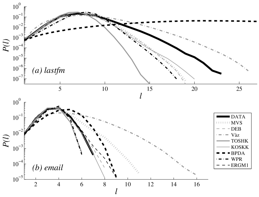
Figure 6: Distributions $P(l)$ of geodesic path lengths $l$ in models fitted to (a) the lastfm data, and (b) the email data. The data is shown as a thick black line in each panel. Averaged over $100$ network realizations.

4.4 Community structure

Cliques

Finally, we assess the community structure of the networks. Perhaps the simplest possible measure of community structure is the number of cliques (Fig. 8a), or fully connected subgraphs, of different sizes. Figure 7 displays the average numbers of cliques in the model networks. Because each network has roughly an equal number of nodes and links, the different numbers of cliques are due to the arrangement of links within the network and not to differences in global link density. It turns out that the NAMs produce clique size distributions that match the data sets fairly well in both fits. The WPR model, fitted to the email data, is shown in Fig. 7. The KOSKK and DEB models also produce distributions roughly comparable to the empirical data, and the Váz model in fact produces far too many large cliques when link density is high (Fig. 7). The MVS and TOSHK models have trouble producing large enough cliques when link density is low (the lastfm fits). A possible explanation of why the MVS model produces very few cliques is indicated by the comparison of Section 4.5, where node deletion is seen to preserve more cliques than link deletion. The parametrization of the TOSHK model, requiring that the number of secondary contacts be drawn from a uniform distribution, severely limits the number of coincident triangles and hence cliques which can be formed. The ERGM1 model produces the fewest cliques of all the models.

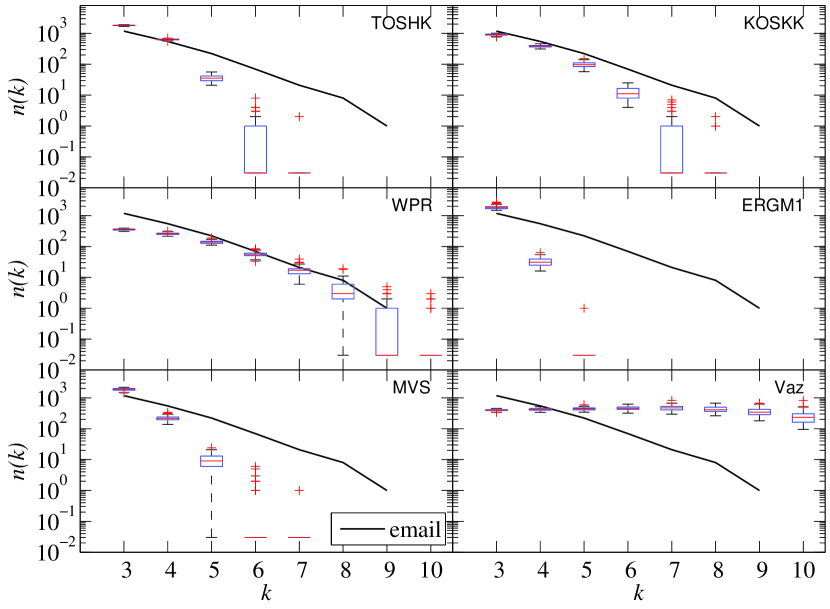
Figure 7: Number $n(k)$ of cliques of size $k$ in the model networks fitted to the email data, shown as a solid line in each panel for reference. Cliques within larger cliques, such as triangles within a $4$-clique, are not counted. Averaged over $100$ network realizations.

k-clusters

We also identify communities using the k-clique-percolation method developed by Palla et al. (2005). The method defines a k-cluster as a subgraph within which all nodes can be reached by ’rolling’ a $k$-clique such that all except one of its nodes are fixed (see Fig. 8b). Figure 9 displays the size distributions of $k$-clusters with $k=4$ and $k=5$ for several models fitted to the email data. As the ERGM1 model produced very few cliques apart from triangles, it cannot generate large $k$-clusters for $k>3$. The other models generally produce $4$-cluster size distributions roughly matching the data, but large $5$-clusters are relatively few. The Váz model generates networks containing very large $k$-clusters with high values of $k$. These are likely due to an extremely dense ’core’ formed around nodes that joined the network early on. For example, each of the $100$ network realizations contained $10$-cluster of size $s=72\pm 15$ (not shown). Such dense clusters are not generally observed in empirical data. For example, in the lastfm and email data sets, the largest $10$-clusters are of sizes $10$ and $12$, respectively.

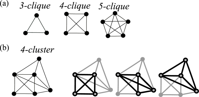
Figure 8: (a) $k$-cliques for $k=3,4,5$. (b) An example of a $4$-cluster with $6$ nodes, highlighting the $4$-cliques from which it is formed.

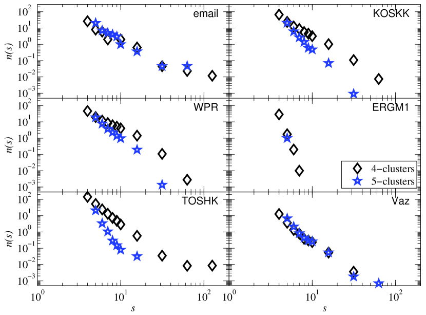
Figure 9: Average number $n(s)$ of $k$-clusters of size $s$ in a network, for $k=4$ ($\diamond$) and $k=5$ ($\star$), in the email data, and in models fitted to it. Averaged over $100$ network realizations.

Role of links with low overlap

In both of our empirical networks, as well as in the networks generated by the studied models, a rather large fraction of edges does not participate in any triangles. In the lastfm and email data, the fraction of such edges is $31.2\%$ and $22.4\%$ respectively. The DEB, TOSHK, Váz, and ERGM1 models produce slightly too few such links ($20$ to $22\%$ in the the lastfm fits and $4$ to $5\%$ in the email fits, except $12,6\%$ in the email fit of ERGM1), whereas the nodal attribute models and KOSKK tend to generate slightly too many of them ($35$ to $40\%$ in the the lastfm fits and $27$ to $41\%$ in the email fits).

We can ask what structural role is played by links that do not participate in triangles, or more generally, by links whose end nodes share only a small fraction of their neighbors. Within a community, adjacent nodes tend to share many neighbors, while for edges between communities, the neighborhoods of the end nodes will not overlap much. This can be quantified using a measure called the overlap $O_{ij}$ (Onnela et al., 2007b), which could be interpreted as a modification of the edgewise shared partners measure (Hunter, 2007), measuring the fraction instead of the number of edgewise shared partners for the end nodes of an edge. The measure also bears resemblance to the Jaccard coefficient (Jaccard, 1901). The overlap is defined as $O_{ij}=\frac{n_{ij}}{(k_{i}-1)+(k_{j}-1)-n_{ij}}$, where $n_{ij}$ is the number of neighbors common to both nodes $i$ and $j$, and $k_{i}$ and $k_{j}$ are their degrees (Fig. 10).

Figure 10: Overlap $O_{ij}$ of edge $e_{ij}$.

Removing low-overlap-links will separate dense, loosely interconnected communities from one another. This turns out to discern the nodal attribute models and the KOSKK model from the other models and our empirical data. Figure 11(a) displays the relative sizes of the largest component after removing links that do not participate in triangles for the lastfm data and the models fitted to it. The nodal attribute models break down to small clusters, whereas in the other models a large core remains.

As noted earlier, the NAMs contain more zero-overlap links than the other models. Hence, it is useful to check whether their breakdown was due to a larger fraction of removed links. We can test this by removing an equal fraction of links from all networks ($41\%$, the maximum fraction of links removed from any network when only non-triangle-links were removed) (Fig. 11b). We remove links in increasing order of overlap $O_{ij}$. Again, a core remains intact in most of the NEMs, whereas the NAMs and the KOSKK network break down, indicating in these models the absence of a core, and the role of low overlap links as bridges between clusters.

The link densities of the remaining components, $d=2\;l/s(s-1)$, where $s$ is the number of nodes in the component and $l$ the number of links, are moreover observed to be slightly higher in the NAMs than in the other models, despite the fact that more links were removed from them (not shown). The above findings show that these networks consist of very clear communities that are loosely interconnected. The other NEMs and ERGM1 on the other hand contain a core that does not consist of such loosely connected clusters. This difference is depicted schematically in Fig. 11(c,d).

Figure 11: (a) Relative size $R_{LC}$ of the largest connected component in the models fitted to the lastfm data after removing links with overlap $O=0$. (b) To show that the breakdown of the nodal attribute models was not simply due to a larger number of links removed, we now remove the same fraction of the lowest overlap links from all models and data ($41\%$, the maximum fraction removed in Fig. 11(a)). Data averaged over $100$ network realizations. (c and d) Schematic depiction of the structural differences related to links with low overlap (links whose end nodes share only a small fraction of their neighbors). (c) Low overlap links connect small, relatively tightly bound clusters together. (d) The network contains a core that does not disintegrate when low overlap links are removed.

In the email fits, link density in the network is higher, and for all networks slightly larger overlap links need to be removed in order to decompose them to small clusters (not shown), but the general difference between the NEMs and NAMs remains. As the ERGM1 model was only fitted to the email data, it is not displayed in Fig. 11. Removing low overlap links did not reduce the largest component of the ERGM1 networks practically at all - even after removing $50$ percent of links beginning with lowest overlap, a core containing on average $93.6$ percent of the nodes remains intact - consistently with the finding that the networks did not contain many denser substructures such as cliques or $k$-clusters.

4.5 Differences in network structure resulting from choice of mechanisms for triadic closure and link deletion

Here, we will examine the differences in network structure resulting from combinations of the mechanisms of link generation (T1,T2) and deletion (ND,LD) emplyed in dynamical network evolution models. Taking as a starting point the simplest of the dynamical models (DEB), in which a newcomer will link to exactly two uniformly randomly chosen nodes, after which it will only initiate triadic closure steps, we study all four combinations of the mechanisms (Fig. 12, a). Two findings speak in favor of using the node deletion mechanism: The model variants using T1 show a clearly assortative relation, suitable for social network models, whereas the T2 networks are dissortative or very weakly assortative (Fig. 12, b). Node deletion also preserves more cliques in the network, a desirable feature for social networks (Fig. 12, c). The larger number of cliques preserved by node deletion is not explained by the clustering coefficients, which turned out to be similar in all networks. The parameters were selected such that $N_{LC}$ and $\bar{k}$ matched the lastfm data.

The choice of triangle generation mechanism, on the other hand, is seen to affect the degree distribution. Networks generated with the T1 mechanism have higher degree nodes than those using the T2 mechanism (Fig. 12, d). This is because following a link is more likely to lead to a high degree node than picking a node randomly. Because in T1 both of the nodes gaining a link in the triad formation step are chosen by following a link, high degree nodes obtain more additional links than when the T2 mechanism is used, in which one of the nodes is chosen randomly. The choice of T1 or T2 does not seem to have an effect on the number or size of cliques generated, nor on degree-degree correlations.

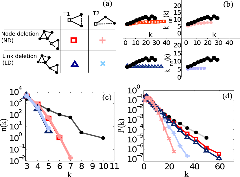
Figure 12: Comparison of mechanisms employed in dynamical network evolution models. (a) Two mechanisms of triadic closure (T1 and T2) are combined with two ways of deleting links (node deletion refers to deleting all links of a node, and link deletion refers to deleting randomly selected links). The same symbols are used in panels (b)-(d). (b) Average nearest neighbor degree $\overline{k_{nn}}$ with respect to node degree $k$, variants arranged as in the schematic figure. The lastfm data is also shown in each panel. (c) Number $n(k)$ of cliques of each size $k$. Smaller cliques within larger cliques are not counted. (d) Degree distribution $P(k)$. Averaged over $100$ network realizations.

5 Summary and discussion

In order to assess the resemblance to empirical networks of the many models for social networks that have been published in recent years in the physics-oriented complex networks literature, we have fitted these models to empirical data and assessed their structure. We have also compared these models with an exponential random graph model that incorporates recently proposed specifications, in the first systematic comparison between models from these families. In addition to comparing structural features of networks produced by the models, we have discussed the different philosophies underlying the model types.

The structural features we focused on are similar in the two included empirical data sets as in numerous other large empirical social networks (Onnela et al., 2007b; Seshadri et al., 2008; Leskovec and Horvitz, 2008) in that they have highly skewed degree distributions, high average clustering coefficients, decreasing clustering spectra $c(k)$, and positive degree-degree-correlations $r$. Therefore, any widely applicable model for social networks should be able to approximately reproduce the average values and distributions of their main characteristic features. However, as the philosophy behind the NEMs studied here is to explain the emergence of common structural features of social networks, we shouldn’t expect them to capture perfectly all features of particular empirical data sets. Our main motivation for fitting the models to the selected target features was to unify approximately some of their properties, in order to compare meaningfully their higher order properties, such as the degree distribution and community structure. These are not likely to be drastically altered by small differences in the average values. Hence, we do not consider an accurate fit in the average quantities of extreme importance.

For almost all models, we saw that average largest component size $\overline{N_{LC}}$ and average degrees $\bar{k}$ could be fitted closely to both empirical data sets. In the ERGM1 model, we compromized matching average degree in order to obtain a reasonable clustering coefficient. Adaptability was limited by the number of free parameters. The models DEB and Váz, which had only one free parameter in addition to network size, turned out to have excessively high average clustering coefficients even for the moderate average degrees displayed by our two data sets. For most of the other models, clustering could be tuned rather closely. Being able to match the targeted average values of these two data sets does not guarantee that a model is able to match those features in other empirical data, however. In this sense, the generalisability of conclusions based on only two data sets is limited.

Table 7: Summary of structural properties of networks generated with the studied models.

Property	lastfm and email	NAMs	dynamical NEMs	growing NEMs	ERGM1
degree distribution	relatively broad	peaked	relatively broad	broad	relatively broad
clustering spectrum	decreasing	flat	decreasing	decreasing	decreasing
assortativity	yes	yes (high)	yes (weak)	yes (moderate/high)	yes (weak)
geodesic path lengths	-	in 1D, too long longest paths	reasonable	reasonable	reasonable
cliques	many large cliques	many large cliques	many in KOSKK, fewest in MVS	too few in TOSHK, exceedingly in Váz	very few
$k$-clusters	many large $k$-clusters for $k=4$ and $k=5$	reasonable	reasonable in DEB and KOSKK, too few in MVS	in Váz, exceedingly large $k$-clusters with large $k$	no large $k$-clusters
consisting of dense clusters interconnected by low-overlap links	no	yes	yes (KOSKK), no (DEB and MVS)	no	no

Table 7 summarizes the structural features in networks resulting from the different model types. Nodal attribute models (NAMs) in which the nodes are located with uniform probability in the underlying social space and links are based solely on homophily, produce a clustering spectrum $c(k)$ strikingly different from observed data, indicating that it is not a sufficient description of the mechanisms at play in the formation of social networks. They also produce peaked degree distributions without very high degree nodes that do no agree with empirical data on large scale social networks. The homophily principle employed in the nodal attribute models is seen to be sufficient for producing strong positive degree-degree correlations. This is a direct result of the dependence of link probability on distance: because high degree nodes appear in locations with a dense population of nodes, their neighbors will also tend to have high degree. The NAMs also generate networks containing a large number of cliques and consisting of dense clusters loosely connected with low overlap links. Their clustered structure appears more pronounced than in the data.

We find that many of the studied network evolution models (NEMs) produce broader degree distributions and decreasing clustering spectra that agree more closely with empirical data. Most of them also generate assortative networks, although typically not to the same extent as in the data, and many large cliques and $k$-clusters. In the dynamical NEMs, node deletion is seen to produce more assortative networks than link deletion. With respect to thresholding by overlap, the dynamical KOSKK model displayed the clearest clustered structure of all the NEMs. This shows that the weights employed in tie formation in the KOSKK model play an important role in the formation of community structure, as the authors observed (Kumpula et al., 2007). The other NEMs produced networks which, in accordance with the data, contained a large core that did not break apart when low overlap links were removed.

The exponential random graph model ERGM1 incorporating recently proposed terms for structural dependencies (Snijders et al., 2006; Hunter et al., 2008; Robins et al., 2007b) was seen to generate very few large cliques. It did produce assortative networks, although with relatively low assortativity. These terms had earlier been employed without difficulty when fitting ERGMs to a large social network (Goodreau, 2007). However, we encountered problems of multimodality with the model.

Very large social networks of millions of individuals, within a country or worldwide, can be assessed with data provided by modern electronic communications, such as mobile phone calls (Onnela et al., 2007a) or instant messaging (Leskovec and Horvitz, 2008). The data have revealed features of large scale networks of human interaction that could not be discerned from a small subnetwork. These include the tails of highly skewed distributions as well as distributions of mesoscale structures, such as the size distribution of communities. Modeling the structure observed in large networks benefits from the ability to generate networks of comparable size. NEMs and NAMs fulfill this requirement.

Using realistic models for social networks in simulation studies of social processes is essential in light of the knowledge that network structure influences many processes (Castellano et al., 2007), such as the emergence and survival of cooperation (Lozano et al., 2008), spreading of information (Onnela et al., 2007a; Moreno et al., 2004) or epidemics (ná and Pastor-Satorras, 2002), and coexistence of opinions (Lambiotte et al., 2007).

Many structural characteristics of social networks were attained even with very simple mechanisms. However, neither the nodal attribute models based on homophily, nor the network evolution models based on triadic closure and global connections, were able to reproduce all important features of social networks. As both mechanisms obviously are present in the evolution social networks, a combination of the model types could yield more realistic network models.

Appendix A Appendix

A.1 Basic network measures

The network representation of social contacts consists of nodes representing the individuals, and links representing the ties between them. An overline is used to denote averaging over all nodes (or links) within the network, or across several networks. We denote by $N$ the number of nodes in a network, i.e. network size. A component of a network is a connected subset of nodes. In this paper, we study the largest component LC of each network. We denote its size by $N_{LC}$. The number of network neighbors of a node is called its degree $k$. An isolated node has degree zero.

A measure of local triangle density, the clustering coefficient, describes the extent to which the neighbors of node $i$ are acquainted with one another: if none on them know each other, $c_{i}$ is zero, while if all of them are acquainted, $c_{i}=1$. For a node $i$ with degree $k_{i}$ and belonging to $T_{i}$ triangles, the clustering coefficient is defined as

$$c_{i}=\frac{T_{i}}{k_{i}(k_{i}-1)/2},$$ (4)

where the denominator ${k_{i}(k_{i}-1)/2}$ expresses the maximum possible number of triangles $i$ could belong to given its degree. The clustering coefficient is not defined for nodes with degree $k<2$. The average clustering coefficient, averaged over all nodes with $k\geq 2$ in the network, is denoted $\bar{c}$. $c(k)$ denotes the average clustering coefficient of nodes with degree $k$. The curve $c(k)$ is called the clustering spectrum.

In large empirical social networks, typically high degree nodes tend to be linked to other high-degree nodes, and low-degree nodes tend to be linked among themselves. One way of quantifying this effect is using linear correlation, or the Pearson correlation coefficient, between the degrees $k_{i}$ and $k_{j}$ of pairs of connected nodes. This is also called the assortativity coefficient $r$ (Newman, 2002):

$$r=\frac{\sum_{e}k_{i}k_{j}/E-\left[\sum_{e}\frac{1}{2}(k_{i}+k_{j})\right]^{2}/E^{2}}{\sum_{e}\frac{1}{2}(k_{i}^{2}+k_{j}^{2})/E-\left[\sum_{e}\frac{1}{2}(k_{i}+k_{j})\right]^{2}/E^{2}},$$

where $E$ is the total number of links in the network. Assortativity can also be quantified using the measure average nearest neighbor degree $\overline{k_{nn}}(k)$, found by taking all nodes with degree $k$, and averaging the degrees of their neighbors. If the curve $\overline{k_{nn}}(k)$ plotted against $k$ has a positive trend, nodes with high degree typically also have high-degree neighbors, and hence the network is assortative.

The geodesic path length $l_{ij}$ between nodes $i$ and $j$ in a network means the minimum number of links that need to be traversed in order to get from $i$ to $j$. The average length $\bar{l}$ of geodesic paths between nodes describes the compactness of the network.

A.2 Determining optimal network parameters

Our fitting method consists of simulating network realizations with different values of the model parameters, and finding the values (points in the parameter space) that produce the best match to the following features of the empirical data sets: average degree $\bar{k}$, average clustering coefficient $\bar{c}$, and average geodesic path lengths $\bar{l}$ (in this order of importance, depending on the number of model parameters). This approach deviates from the tradition of maximum likelihood estimation for fitting probabilistic models.

We attempt to minimize the relative error in each chosen feature. For example, for average degree $\bar{k}$ in a model with given parameter values p, being fitted to a data set with average degree $\overline{k}^{target}$, the relative error is

$$|{\bf\epsilon}_{\overline{k}(\textbf{p})}|=\left|\frac{\overline{k}(\textbf{p})-\overline{k}^{target}}{\overline{k}^{target}}\right|.$$ (5)

The errors for each feature are combined in the error function $f(\textbf{p})$, whose norm $|f(\textbf{p})|$ is minimized. For example, if fitting to $N_{LC}$, $\bar{k}$ and $\bar{c}$, the error function and its norm take the shape

$$f(\textbf{p})=\left[w_{N_{LC}}\epsilon_{N_{LC}}\quad w_{\bar{k}}\epsilon_{\bar{k}}\quad w_{\bar{c}}\epsilon_{\bar{c}}\right],$$ (6)

and its norm

$$|f(\textbf{p})|=\sqrt{w_{N_{LC}}^{2}\epsilon_{N_{LC}}^{2}+w_{\bar{k}}^{2}\epsilon_{\bar{k}}^{2}+w_{\bar{c}}^{2}\epsilon_{\bar{c}}^{2}.}$$ (7)

The error function should have equally many components as there are network parameters. We chose weights that reflected the order of importance given to the targeted features, putting the most emphasis on matching the number of nodes and links, less on clustering, and least on average geodesic path lengths. It turned out that for nearly all of the models (DEB, MVS, KOSKK, Vaz, BPDA, email fit of WPR) the result was insensitive to weights, because the models were able to match the target values closely (up to the number of model parameters). In optimizing the models DEB and KOSKK, we used a linear approximation for the components of the error function, iteratively refining the approximation close to the optimum. For MVS, we used the the well established Nelder-Mead method (Nelder and Mead, 1965), which involves calculating values of the error function at the corners of a simplex (a triangle in 2-dimensional space, a tetrahedron in 3D). The optimal value of the error function is iteratively approached by rolling one corner of the simplex over the others such that the object moves towards the region where the function gets optimal values. The diameter of the simplex is adjusted during iteration to increase accuracy.

Optimization algorithms were not needed for the Váz and BPDA models and the email fit of WPR. For the Váz model, a very good approximation for the optimal value of $u$ can be obtained analytically. This estimate could be refined manually. For the BPDA model, the analytical estimates for $\bar{k}$ and $\bar{c}$ derived by the authors could be used as a starting point in optimization. We refined the initial estimates by first adjusting $\alpha$ to find the correct value for the clustering coefficient, and then changing $b$ until the correct mean degree was found. For small enough adjustments, the latter corrections did not affect the value of $\bar{c}$. The adjustments were done by trial and error, but it was not difficult to get an accurate fit for mean degree and clustering in this manner. For the email fit of WPR, it turned out that $N_{LC}\approx N$, and hence the number of free parameters was reduced. $p$ was set to obtain desired average degree, and the two remaining parameters were optimized by generating networks with a grid of their values.

Exact fits could not be obtained for TOSHK, ERGM1, and the lastfm fit of WPR. For WPR, we used weights $[w_{N_{LC}},w_{k},w_{c},w_{l}]=[4\;4\;2\;1]$ and grid optimization similarly as in the email case, although it was costly in four dimensions. Obtaining values in a grid enabled us to visulize the dependence of the targeted features on the model parameters. It turned out that assortativity and clustering varied closely together, rendering assortativity useless as a fitting target if clustering was used; hence we used average geodesic path lengths, which enabled an optimum to be determined. As the TOSHK model has only one continuous parameter $p$, it suffices to optimize $p$ for all values of the discrete parameter $k$ below some $k_{\max}$, making sure that $k_{\max}$ is large enough. The parameter $p$ was optimized to reach the desired mean degree for each $k$, and the pair $(k,p^{\textrm{opt}}(k))$ that provided the best match to the desired $\bar{c}$ was selected as the optimum. Optimization was carried out with the Matlab optimization toolbox function fminbnd.m, which is based on golden section search and parabolic interpolation.

For the remaining case in which no exact match was found (ERGM1), we attempted using the linear approximation method and Nelder-Mead algorithm described above, as well as other, potentially more robust methods (Elster and Neumaier, 1995; Huyer and Neumaier, 2008), but these failed likely due to multimodality of the probability distribution. Figure 13 illustrates the instability we encountered when attempting to fit the ERGM1 model to the email data. The panels display average degree $\bar{k}$ (a) and average clustering coefficient $\bar{c}$ (b) in networks generated with various values of $\theta_{L}$, with the other parameters kept constant at the values listed in Table 5. For each value of $\theta_{L}$, $60$ network realizations are shown (drawn from MCMC chains with burn-in $5\times 10^{7}$ steps, and 5 realizations taken from each chain at intervals of $10^{7}$). Because $\theta_{L}$ controls the number of random links, an increase in $\theta_{L}$ generally increases average degree and decreases average clustering. However, at roughly $\theta_{L}=-6.961$ we observe a sudden transition into a much denser, less clustered network.

Figure 13: (a) Average degree $\bar{k}$ and (b) average clustering coefficient $\bar{c}$ in networks generated from the model ERGM1 with different values of $\theta_{L}$.

References

- Boguña et al. (2004) Boguña, M., Pastor-Satorras, R., Díaz-Guilera, A., Arenas, A., 2004. Emergence of clustering, correlations, and communities in a social network model. Physical Review E 70, 056122.
- Castellano et al. (2007) Castellano, C., Fortunato, S., Loreto, V., 2007. Statistical physics of social dynamics. Reviews of Modern Physics (in press) (arXiv:0710.3256).
- Davidsen et al. (2002) Davidsen, J., Ebel, H., Bornholdt, S., 2002. Emergence of a small world from local interaction: Modeling acquaintance networks. Physical Review Letters 88, 128701.
- Elster and Neumaier (1995) Elster, C., Neumaier, A., 1995. A grid algorithm for bound constrained optimization of noisy functions. The IMA Journal of Numerical Analysis (IMAJNA) 15, 585–608.
-
Fortunato and Castellano (2008)
Fortunato, S., Castellano, C., 2008. Community structure in graphs. In: Meyers,
R. A. (Ed.), Encyclopedia of Complexity and System Science. Springer.
URL arXiv:0712.2716 - Frank (1991) Frank, O., 1991. Statistical analysis of change in networks. Statistica Neerlandica 45(3), 283 – 293.
- Frank and Strauss (1986) Frank, O., Strauss, D., 1986. Markov graphs. Journal of the American Statistical Association (JASA) 81(395), 832.
- Geyer and Thompson (1992) Geyer, C. J., Thompson, E. A., 1992. Monte carlo maximum likelihood for dependent data. Journal of the American Statistical Association (JASA), Series B (Methodological) 54(3), 657–699.
- Goodreau (2007) Goodreau, S. M., 2007. Advances in exponential random graph (p*) models applied to a large social network. Social Networks 29(2), 231–248.
- Granovetter (1973) Granovetter, M., 1973. The strength of weak ties. American Journal of Sociology 78, 1360–1380.
- Guimerà et al. (2003) Guimerà, R., Danon, L., Díaz-Guilera, A., Giralt, F., Arenas, A., 2003. Self-similar community structure in a network of human interactions. Physical Review E 68, 065103(R).
- Handcock (2003) Handcock, M. S., 2003. Assessing degeneracy in statistical models of social networks. Working Paper no. 39.
-
Handcock et al. (2003)
Handcock, M. S., Hunter, D. R., Butts, C. T., Goodreau, S. M., Morris, M.,
2003. statnet: Software tools for the statistical modeling of network data.
URL http://statnetproject.org -
Handcock et al. (2007)
Handcock, M. S., Hunter, D. R., Butts, C. T., Goodreau, S. M., Morris, M., 12
2007. statnet: Software tools for the representation, visualization, analysis
and simulation of network data. Journal of Statistical Software 24 (1),
1–11.
URL http://www.jstatsoft.org/v24/i01 - Hunter (2007) Hunter, D., 2007. Curved exponential family of models for social networks. Social Networks 29, 216–230.
- Hunter et al. (2008) Hunter, D., Goodreau, S., Handcock, M., 2008. Goodness of fit of social network models. Journal of the American Statistical Association (JASA) 103(481), 248–258.
- Huyer and Neumaier (2008) Huyer, W., Neumaier, A., 2008. Snobfit – stable noisy optimization by branch and fit. ACM Transactions on Mathematical Software 35 (2), 1–25.
- Jaccard (1901) Jaccard, P., 1901. Distribution de la flore alpine dans le bassin des dranses et dans quelques régions voisines. Bulletin de la Société Vaudoise des Sciences Naturelles 37, 241–272.
- Jonasson (1999) Jonasson, J., 1999. The random triangle model. Journal of Applied Probability 36, 852–867.
- Kumpula et al. (2007) Kumpula, J., Onnela, J.-P., Saramäki, J., Kaski, K., Kertész, J., 2007. Emergence of communities in weighted networks. Physical Review Letters 99, 228701.
- Lambiotte et al. (2007) Lambiotte, R., Ausloos, M., Holyst, J., 2007. Majority model on a network with communities. Physical Review E 75, 030101(R).
- Lambiotte et al. (2008) Lambiotte, R., Blondel, V. D., de Kerchove, C., Huens, E., Prieur, C., Smoreda, Z., Dooren, P. V., 2008. Geographical dispersal of mobile communication networks. Physica A 387, 5317–5325.
- Leskovec and Horvitz (2008) Leskovec, J., Horvitz, E., 2008. Planetary-scale views on an instant-messaging network. arXiv:0803.0939.
- Lozano et al. (2008) Lozano, S., Arenas, A., Sánchez, A., 2008. Mesoscopic structure conditions the emergence of cooperation on social networks. Public Library of Science one 3, e1892.
- Marsili et al. (2004) Marsili, M., Vega-Redondo, F., Slanina, F., 2004. The rise and fall of a networked society: A formal model. Proceedings of the National Academy of Sciences (PNAS) (USA) 101, 1439–1442.
- Masuda and Konno (2006) Masuda, N., Konno, N., 2006. Vip-club phenomenon: Emergence of elites and masterminds in social networks. Social Networks 28, 297–309.
- McPherson et al. (2001) McPherson, M., Smith-Lovin, L., Cook, J., 2001. Birds of a feather: Homophily in social networks. Annual Reviews of Sociology 27, 415–444.
- Milgram (1967) Milgram, S., 1967. The small world problem. Psychology Today 2, 60–67.
- Moreno et al. (2004) Moreno, Y., Nekovee, M., Pacheco, A. F., 2004. Dynamics of rumor spreading in complex networks. Physical Review E 69, 066130.
- ná and Pastor-Satorras (2002) ná, M. B., Pastor-Satorras, R., 2002. Epidemic spreading in complex correlated networks. Physical Review E 66, 047104.
- Nelder and Mead (1965) Nelder, J., Mead, R., 1965. A simplex algorithm for function minimization. The Computer Journal 7, 308–313.
- Newman (2001) Newman, M., 2001. The structure of scientific collaboration networks. Proceedings of the National Academy of Sciences (PNAS) (USA) 98, 404.
- Newman (2002) Newman, M., 2002. Assortative mixing in networks. Physical Review Letters 89, 208701.
- Onnela et al. (2007a) Onnela, J.-P., Saramäki, J., Hyvönen, J., Szabó, G., Lazer, D., Kaski, K., Kertész, J., Barabási, A.-L., 2007a. Structure and tie strengths in mobile communication networks. Proceedings of the National Academy of Sciences (PNAS) (USA) 104, 7332.
- Onnela et al. (2007b) Onnela, J.-P., Saramäki, J., Hyvönen, J., Szabó, G., de Menezes, M. A., Kaski, K., Barabási, A.-L., Kertész, J., 2007b. Analysis of a large-scale weighted network of one-to-one human communication. New Journal of Physics 9, 179.
- Palla et al. (2005) Palla, G., Derényi, I., Farkas, I., Vicsek, T., 2005. Uncovering the overlapping community structure of complex networks in nature and society. Nature 435, 814–818.
- Robins et al. (2007a) Robins, G., Pattison, P., Kalish, Y., Lusher, D., 2007a. An introduction to exponential random graph (p*) models for social networks. Social Networks 29, 173–191.
- Robins et al. (2007b) Robins, G., Snijders, T., Wang, P., Handcock, M., Pattison, P., 2007b. Recent developments in exponential random graph (p*) models for social networks. Social Networks 29, 192–215.
- Seshadri et al. (2008) Seshadri, M., Machiraju, S., Sridharan, A., Bolot, J., Faloutsos, C., Leskovec, J., 2008. Mobile call graphs: beyond power-law and lognormal distributions. Proceedings of the 14th ACM SIGKDD international conference on Knowledge discovery and data mining, Las Vegas, Nevada, USA, 596–604.
- Snijders et al. (2006) Snijders, T., Pattison, P., Robins, G., Handcock, M., 2006. New specifications for exponential random graph models. Sociological Methodology 36(1), 99–153.
- Snijders (1996) Snijders, T. A. B., 1996. Stochastic actor-oriented dynamic network analysis. Journal of Mathematical Sociology 21, 149–172.
- Snijders (2001) Snijders, T. A. B., 2001. The statistical evaluation of social network dynamics. In: Sobel, M., Becker, M. (Eds.), Sociological Methodology. Boston and London: Basil Blackwell.
- Snijders (2002) Snijders, T. A. B., 2002. Markov chain monte carlo estimation of exponential random graph models. Journal of Social Structure 3 (2).
- Toivonen et al. (2006) Toivonen, R., Onnela, J.-P., Saramäki, J., Hyvönen, J., Kaski, K., 2006. A model for social networks. Physica A 371(2), 851–860.
- Vázquez (2003) Vázquez, A., 2003. Growing networks with local rules: Preferential attachment, clustering hierarchy, and degree correlations. Physical Review E 67, 056104.
- Wasserman and Pattison (1996) Wasserman, S., Pattison, P., 1996. Logit models and logistic regressions for social networks, i. an introduction to markov graphs and p *. Psychometrika 61, 401–425.
- Wong et al. (2006) Wong, L. H., Pattison, P., Robins, G., 2006. A spatial model for social networks. Physica A 360, 99–120.