Inferring coupling strength from event-related dynamics

Abstract

We propose an approach for inferring strength of coupling between two systems from their transient dynamics. This is of vital importance in cases where most information is carried by the transients, for instance in evoked potentials measured commonly in electrophysiology. We show viability of our approach using nonlinear and linear measures of synchronization on a population model of thalamocortical loop and on a system of two coupled Rössler-type oscillators in non-chaotic regime.

I Introduction

Coherent actions of apparently distinct physical systems often provoke questions of their possible interactions. Such coherence in interacting systems is often a result of their synchronization Pikovsky et al. (2001). It became a popular topic with the discovery of synchronization of non-identical chaotic oscillators Pecora and Carroll (1990). Over the years different types of synchrony were studied, notably phase synchronization Rosenblum et al. (1996). There were also numerous attempts to study more complicated interactions under the names of generalized synchronization or interdependence Rulkov et al. (1995); Pecora et al. (1995); Kocarev and Parlitz (1996); Schiff et al. (1996); Wójcik et al. (2001). In biological context synchronization is expected to play a major role in cognitive processes in the brain Rosenblum et al. (2001); Singer and Gray (1995); Varela et al. (2001) such as visual binding Singer and Gray (1995) and large-scale integration Varela et al. (2001). Various synchronization measures were successfully applied to electrophysiological signals Arnhold (1999); Kamiński et al. (2001); Varela et al. (2001); Quiroga et al. (2002); Niebur et al. (2002); Angelini et al. (2004); Lai et al. (2007); Korzeniewska et al. (2007). In this work we concentrate on nonlinear interdependence Arnhold (1999); Quiroga et al. (2002).

For an experimentalist it is often interesting to know how two systems synchronize during short periods of evoked activity Fell et al. (2001); Kramer et al. (2004). Such questions arise naturally in analysing data from animal experiments Kublik et al. (2003); Kublik (2004); Świejkowski (2007); Wróbel et al. (2007). One measures there electrical activity on different levels of sensory information processing and aims at relating changes in synchrony to the behavioral contex, such as attention or arousal. It may be the case that the stationary dynamics (with no sensory stimulation) corresponds to a fixed point. For instance, when one measures the activity in the barrel cortex of a restrained and habituated rat, the recorded signals seem to be noise Kublik et al. (2003); Kublik (2004); Świejkowski (2007). On the other hand transient activity evoked by specific stimuli seems to provide useful information. For example, bending a bunch of whiskers triggers non-trivial patterns of activity (evoked potentials, EPs) in both the somatosensory thalamic nuclei and the barrel cortex Świejkowski (2007); Łęski et al. (2007).

Explorations described in this paper aim at solving the following problem. Suppose we have two pairs of transient signals, for example recordings of evoked potentials from thalamus and cerebral cortex in two behavioral situations Kublik et al. (2003); Świejkowski (2007). Can we tell in which of the two situations the strength of coupling between the structures is higher? Thus we investigate if one can measure differences in the strength of coupling between two structures using nonlinear interdependence measures on an ensemble of EPs. Since EPs are short, transient signals, straightforward application of the measures motivated by studies of systems moving on the attractors (stationary dynamics) is rather doubtful and a more sophisticated treatment is needed Andrzejak et al. (2006); Kramer et al. (2004). Our approach is similar in spirit to that advocated by Janosi and Tel for the reconstruction of chaotic saddles from transient time series Jánosi and Tél (1994). (Note that the transients we study should not be confused with the transient chaos studied by Janosi and Tel.) Thus we cut pieces of the recordings corresponding to well-localized EPs and paste them together one after another. Since we are interested in the coupled systems, unlike Janosi and Tel, we obtain two artificial time-series to which we then apply nonlinear interdependence measures and linear correlations. It turns out that this approach allows to extract the information about the strength of the coupling between the two systems.

We test our method on a population model of information processing in

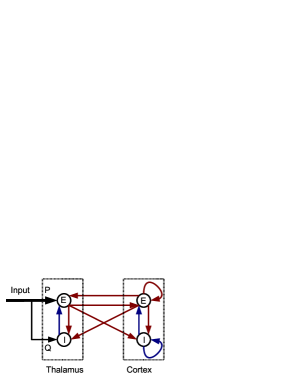
Figure 1: Structure of the model of the thalamocortical loop used in the simulations.

thalamocortical loop (Figure 1) consisting of two coupled Wilson-Cowan structures Wilson and Cowan (1972, 1973). Sensory information is relayed through thalamic nuclei to cortical fields, which in return send feedback connections to the thalamus. This basic framework of the early stages of sensory systems is to a large extent universal across different species and modalities Shepherd (2004). To check that the results are not specific to this particular system we also study evoked dynamics of two coupled Rössler-type oscillators in non-chaotic regime.

The paper is organized as follows. In Sec. II we define the measures to be used. In Sec. III we describe the models used to test our method. Our model of thalamocortical loop is discussed in Sec. III.1 and a system of two coupled Rössler-type oscillators is described in Sec. III.2. In Sec. IV we present the results. In Sec. IV.1 we show how various interdependence measures calculated on the transients are related to the coupling between the systems, while in Sec. IV.2 we study how the resolution of our methods degrades with noise. Finally, in Sec. IV.3, we apply time-resolved interdependence measure $H_{i}$ Andrzejak et al. (2006) and compare its utility with our approach. We summarize our observations in Sec. V.

II Synchronization measures

In the present paper we mainly study the applicability of nonlinear interdependence measures on the transients. These measures, proposed in Arnhold (1999), are non-symmetric and therefore can provide information about the direction of driving, even if the interpretation in terms of causal relations is not straightforward Quiroga et al. (2000).

These measures are constructed as follows. We start with two time series $x_{n}$ and $y_{n}$, $n=1,\ldots,N$, measured in systems $\mathrm{X}$ and $\mathrm{Y}$. We then construct $m$-dimensional delay-vector embeddings Takens (1980) $\mathbf{x}_{n}=(x_{n},\ldots,x_{n-(m-1)\tau})$, similarly for $\mathbf{y}_{n}$, where $\tau$ is the time lag. The information about the synchrony is inferred from comparing the size of a neighborhood of a point in $m$-dimensional space in one subsystem to the spread of its equal-time counterpart in the other subsystem. The idea behind it is that if the systems are highly interdependent then the partners of close neighbors in one system should be close in the other system. Several different measures exploring this idea can be considered depending on how one measures the size of the neighborhood. These variants include measures denoted by $S$, $H$ Arnhold (1999), $N$ Quiroga et al. (2002), $M$ Andrzejak et al. (2003). We have studied the properties of most of these measures but for the sake of clarity here we report only the results for the “robust” variant $H$ and a normalized measure $N$, as they proved most useful for our purposes.

Let us, following Arnhold (1999), for each $\mathbf{x}_{n}$ define a measure of the spread of its neighborhood equal to the mean squared Euclidean distance:

$$R^{(k)}_{n}(\mathrm{X})=\frac{1}{k}\sum_{j=1}^{k}(\mathbf{x}_{n}-\mathbf{x}_{r_{n,j}})^{2},$$

where $r_{n,j}$ are the time indices of the $k$ nearest neighbors of $\mathbf{x}_{n}$, analogously, $s_{n,j}$ denotes the time indices of the $k$ nearest neighbors of $\mathbf{y}_{n}$. To avoid problems related to temporal correlations Theiler (1986), points closer in time to the current point $\mathbf{x}_{n}$ than a certain threshold are typically excluded from the nearest-neighbor search (Theiler correction). Then we define the $\mathbf{y}$-conditioned mean

$$R^{(k)}_{n}(\mathrm{X}|\mathrm{Y})=\frac{1}{k}\sum_{j=1}^{k}(\mathbf{x}_{n}-\mathbf{x}_{s_{n,j}})^{2},$$

where the indices $r_{n,j}$ of the nearest neighbors of $\mathbf{x}_{n}$ are replaced with the indices $s_{n,j}$ of the nearest neighbors of $\mathbf{y}_{n}$. The definitions of $R^{(k)}_{n}(\mathrm{Y})$ and $R^{(k)}_{n}(\mathrm{Y}|\mathrm{X})$ are analogous. The measures $H$ and $N$ use the mean squared distance to random points:

$$R_{n}(\mathrm{X})=\frac{1}{N-1}\sum_{j\neq n}(\mathbf{x}_{n}-\mathbf{x}_{j})^{2},$$

and are defined as

$$H^{(k)}(\mathrm{X}|\mathrm{Y}) = \frac{1}{N}\sum_{n=1}^{N}\log\frac{R_{n}(\mathrm{X})}{R^{(k)}_{n}(\mathrm{X}|\mathrm{Y})},$$

$$N^{(k)}(\mathrm{X}|\mathrm{Y}) = \frac{1}{N}\sum_{n=1}^{N}\frac{R_{n}(\mathrm{X})-R^{(k)}_{n}(\mathrm{X}|\mathrm{Y})}{R_{n}(\mathrm{X})}.$$

The interdependencies in the other direction $H^{(k)}(\mathrm{Y}|\mathrm{X})$, $N^{(k)}(\mathrm{Y}|\mathrm{X})$ are defined analogously and need not be equal $H^{(k)}(\mathrm{X}|\mathrm{Y})$, $N^{(k)}(\mathrm{X}|\mathrm{Y})$.

Such measures base on repetitiveness of the dynamics: one expects that if the system moves on the attractor the observed trajectory visits neigborhoods of every point many times given sufficiently long recording. The same holds for the reconstructed dynamics. However, if the stationary part of the signal is short or missing, especially if we observe a transient such as evoked potential, this is not the case. Still, if we have noisy dynamics, every repetition of the experiment leads to a slightly different probing of the neighborhood of the noise-free trajectory. This observation led us to an idea of gluing a number of repetitions of the same evoked activity (with different noise realizations) together and using such pseudo-periodic signals as we would use trajectories on a chaotic attractor. A similar idea was used by Janosi and Tel in a different context for a different purpose Jánosi and Tél (1994). An example of a delay embedding of a signal obtained this way is presented in Fig. 2. Note that artifacts may emerge at the gluing points. This is discussed in Jánosi and Tél (1994), and some countermeasures are proposed. For simplicity we proceed with just gluing as we expect that the artifacts only increase the effective noise level. The influence of noise is studied in Sec. IV.2.

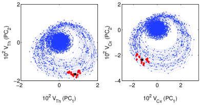
Figure 2: Delay-vector embeddings (shown in planes defined by the first two principal components) of pseudo-periodic signals obtained by gluing 50 evoked potentials generated in a model of thalamocortical loop. On the left (signal from “thalamus”) a point is chosen (black square) and its 15 nearest neighbors are marked with red (gray) diamonds. On the right (“cortex”) the equal-time partners of the marked points from the left picture are shown.

Recently, time-resolved variants of the methods described above were studied Kramer et al. (2004); Andrzejak et al. (2006). They are applied to ensembles of simultaneous recordings, each consisting of many different realizations of the same (presumably short) process. Let us denote the $n$-th state vector in $j$-th realization of the time-series by $\mathbf{x}^{j}_{n}$ ($\mathbf{y}^{j}_{n}$, respectively), $j=1,\ldots,J$. The idea in Kramer et al. (2004) is, for given $\mathbf{x}^{j}_{n}$ to find one neighbor in each of the ensembles. Then a measure (denoted $T$) based on distances to these neighbors is constructed. The proposition of Andrzejak et al. (2006) is to look not at the nearest neighbors of a given $\mathbf{x}_{n}$ no matter what time they occur at, but rather at the spread of state-vectors at the same latency across the ensemble. In Sec. IV.3 we study the measure $H_{i}$ as defined in Andrzejak et al. (2006). Let $r_{i}^{j,l}$ denote the ensemble index of the $l$-th nearest neighboor of $\mathbf{y}_{n}^{j}$ among the whole ensemble $\{\mathbf{y}^{j}_{n}\}^{j=1,\ldots J}$. Define the quantities

$$R^{j,(k)}_{i}(\mathrm{X}|\mathrm{Y}) = \frac{1}{k}\sum_{l=1}^{k}(\mathbf{x}_{i}^{j}-\mathbf{x}_{i}^{r^{j,l}_{i}})^{2},$$

$$R^{j,(k)}_{i}(\mathrm{X}) = \frac{1}{J-1}\sum_{s\neq j}(\mathbf{x}_{i}^{j}-\mathbf{x}_{i}^{s})^{2}.$$

The time-resolved interdependence measure is further defined as

$$H^{(k)}_{i}(\mathrm{X}|\mathrm{Y})=\frac{1}{J}\sum_{j=1}^{J}\log\frac{R^{j,(k)}_{i}(\mathrm{X})}{R^{j,(k)}_{i}(\mathrm{X}|\mathrm{Y})}.$$

Analogously one can define $H^{(k)}_{i}(\mathrm{Y}|\mathrm{X})$ and also time-resolved variants of other interdependence measures.

In the numerical experiments described in this paper we use the following parameters of the nonlinear interdependence measures: time lag for construction of delay-vectors: $\tau=1$, embedding dimension $m=10$, number of nearest neighbors $k=15$, Theiler correction $T=5$. To calculate the interdependencies we used the code by Rodrigo Quian Quiroga and Chee Seng Koh available at http://www.vis.caltech.edu/~rodri/Synchro/Synchro_home.htm. In case of the measure $H_{i}$ we use the same embedding dimension and time lag; here $k=1$. To calculate this measure we used the code provided in supplementary material to Andrzejak et al. (2006). To compare the linear and nonlinear analysis methods we calculated the cross-correlation coefficients using Matlab.

While in numerical studies the correctness of reconstruction can often be easily checked by comparison with original dynamics, in analysis of experimental data it can be a complex issue. Correct reconstruction is a prerequisite for application of our technique. For technical details on best practices of delay embedding reconstructions, pitfalls and caveats, see Kantz and Schreiber (2004).

III Model data

III.1 Connected Wilson-Cowan aggregates

Our model of the thalamocortical loop was based on the Wilson and Cowan mean-field description of interacting populations of excitatory and inhibitory neural cells Wilson and Cowan (1972, 1973). In the simplest version, which we used, each population is described by a single variable standing for its mean level of activity

$$\begin{split}\tau_{E}\frac{\mathrm{d}E}{\mathrm{d}t}&=-E+(k_{E}-r_{E}E)\mathcal{S}_{E}(c_{EE}E-c_{IE}I+P),\\ \tau_{I}\frac{\mathrm{d}I}{\mathrm{d}t}&=-I+(k_{I}-r_{I}I)\mathcal{S}_{I}(c_{EI}E-c_{II}I+Q).\end{split}$$ (1)

The variables $E$ and $I$ are the mean activities of excitatory and inhibitory populations, respectively, and form the phase space of a localized neuronal aggregate. The symbols $\tau$, $k$, $r$, $c$ denote parameters of the model, $\mathcal{S}$ are sigmoidal functions, $P$ and $Q$ are input signals to excitatory and inhibitory populations, respectively. These equations take into account the absolute refractory period of neurons which is a short period after activation in which a cell cannot be activated again. Such models exhibit a number of different behaviors (stable points, hysteresis, limit cycles) depending on the exact choice of parameters Wilson and Cowan (1972, 1973). To relate the simulation results to the experiment Kublik et al. (2003); Świejkowski (2007) we considered the observable $V=E-I$, since the electric potential measured in experiments is related to the difference between excitatory and inhibitory postsynaptic potentials (see the discussion in Wilson and Cowan (1972)).

We studied a model composed of two such mutually connected aggregates, which we call “thalamus” and “cortex” (Figure 1). Note that the parameters characterizing the two parts are different (see the Appendix A for a complete specification of the model). Specifically, there are no excitatory-excitatory nor inhibitory-inhibitory connections in the thalamus. Only the thalamus receives sensory input, and we assume that $Q$ is always a constant fraction of $P$. The connections between two subsystems are excitatory only.

To model the stimulus we assumed that the input ($P,Q$) switches at some point from 0 to a constant value ($P_{C},Q_{C}$), and after a short time (on the time-scale of relaxation to the fixed point) switches back to zero. This is clearly another simplification, as the real input, which could be induced by bending a bunch of whiskers Kublik et al. (2003); Kublik (2004); Świejkowski (2007), would be a more complex function of time. However, the transient nature of the stimulus is preserved. In this simple setting we can understand that the “evoked potential” corresponds to a trajectory approaching the asymptotic solution of the “excited” system (with the non-zero input $P_{C},Q_{C}$), followed by a relaxation to the “spontaneous activity” in the system with null input.

The model parameters were chosen so that its response to brief stimulation were damped oscillations of $V$ both in the thalamus and the cortex similar to those observed in the experiments, both in terms of shape and time duration Kublik et al. (2003); Kublik (2004); Świejkowski (2007) (Figure 3). However, apart from that, we exercised little effort to match the response of the model to the actual activity of somatosensory tract in the rat brain. Our main goal in the present work was establishing a method of inferring coupling strength from transients and not a study of the rat somatosensory system. For this reason it was convenient to use a very simplified, qualitative model. Interestingly, the response of the model, measured for example as the activity of excitatory cells in the thalamus, extends in time well beyond the end of the stimulation (Figure 3). Such behavior is not observed in a single aggregate and requires at least two interconnected structures Wilson and Cowan (1973).

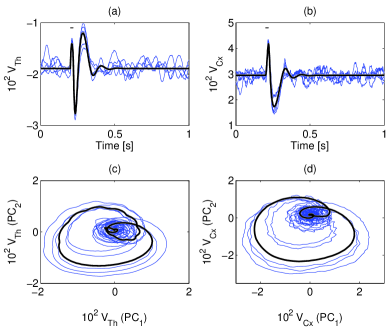
Figure 3: “Evoked potentials” ($V=E-I$), (a), (b) and their delay-vector embeddings shown in a plane defined by the first two principal components (c), (d). Plots (a) and (c): thalamus, (b) and (d): cortex. The intervals above the EP indicate the duration of the non-zero stimulus. Black (thick) lines are solutions for the system without noise, blue (thin) curves are five different realisations of noisy dynamics.

We performed numerical simulations in three modes: either stationary (null or constant input), or not (transient input). The dynamics of the model is presented in Figure 4.

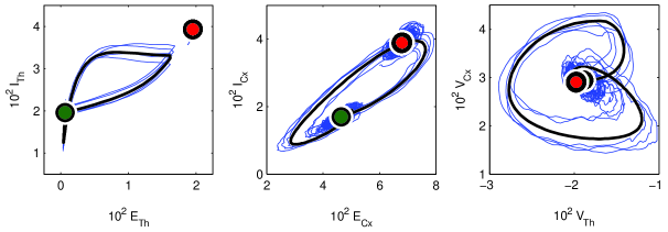
Figure 4: Dynamics of the model. The green (lower left) and red (upper right) dots are fixed points in case of null or constant stimulation respectively, the black (thick) line is the noise-free transient dynamics. Blue (thin) lines are example trajectories of the model in the presence of noise. The plots show projections of the same dynamics to different planes.

In case of transient input the simulation was done for $-1000\leq t\leq 1000$ms. We used the stimulus $P$ and $Q$ which was 0 except for the time $200<t<220$ when it was $P_{C}=3.5$ and $Q_{C}=0.3$. The system settled in the stationary state during the initial segment ($t<195$) which was discarded from the analysis. The noise was simulated as additional input to each of the four populations, see the Appendix A for the equations. For each population we used different Gaussian (mean $\mu=0$, standard deviation $\sigma=0.025$) white noise, sampled at 1kHz and interpolated linearly to obtain values for intermediate time points. In case of stationary dynamics we simulated longer periods, $-1000\leq t\leq 20000$ms. The signals were sampled at 100Hz before the synchronization measures were applied.

In case of constant or null stimulation the system approaches one of the two fixed-point solutions which are marked by large dots in Figure 4. For the amount of noise used here the dynamics of the system changes as expected: the fixed points become diffused clouds (Figure 4). During the transient — “evoked potential” — the switching input forces the system to leave the null-input fixed point, approach the constant-input attractor, and then relax back to its original state (Figure 4). Of course, in the presence of noise the shape of the transient is affected (Figure 4). Observe the similarity between the embedding reconstructions of the evoked potentials (Figure 3, bottom row) and the actual behavior in $V_{\text{Th}}$-$V_{\text{Cx}}$ coordinates (Figure 4, bottom row).

III.2 Coupled Rössler-type oscillators

While we are specifically interested in the dynamics of thalamocortical loop which dictated our choice of the studied system, we checked if our approach is not specific to this model. Our second model of choice consisted of two coupled Rössler-type oscillators Rosenblum et al. (1996); Letellier and Rössler (2006)

$$\frac{\mathrm{d}x_{1}}{\mathrm{d}t} = -(1+\Delta\omega)y_{1}-z_{1}+\alpha C(x_{2}-x_{1})+\xi_{1},$$

$$\frac{\mathrm{d}y_{1}}{\mathrm{d}t} = (1+\Delta\omega)x_{1}-0.15y_{1}+P+\xi_{2},$$

$$\frac{\mathrm{d}z_{1}}{\mathrm{d}t} = 0.2+z_{1}(x_{1}-10)+\xi_{3},$$

$$\frac{\mathrm{d}x_{2}}{\mathrm{d}t} = -(1-\Delta\omega)y_{2}-z_{2}+\alpha C(x_{1}-x_{2})+\xi_{4},$$

$$\frac{\mathrm{d}y_{2}}{\mathrm{d}t} = (1-\Delta\omega)x_{2}-0.15y_{2}+\xi_{5},$$

$$\frac{\mathrm{d}z_{2}}{\mathrm{d}t} = 0.2+z_{2}(x_{2}-10)+\xi_{6}.$$

We used the frequency detuning parameter $\Delta\omega=0.05$ and the maximum coupling constant $C=0.06$. The scaling parameter $\alpha$ took values from $0$ to $1$. The stimulation parameter $P$ was $0$ except for $200<t<250$ where it was set to $0.8$; the noise inputs $\xi_{i}$, $i=1\ldots 6$ were Gaussian white noise with parameters as for the Wilson-Cowan model. The simulation was done for $t\in[0,300]$ and segments from $t=195$ to $t=300$, sampled every $\Delta t=0.125$, were used for the analysis of the transients. The synchronization was measured between $x_{1}$ and $x_{2}$. Parameters of the system were chosen so that asymptotically it moved into a stable fixed point (note the signs in the equations for ${y_{1}}$ and ${y_{2}}$) for both $P=0$ and $P=0.8$. Therefore the transient dynamics (Fig. 5)

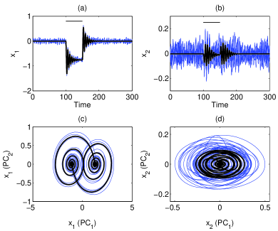
Figure 5: (a), (b): signals ($x$ coordinate) from coupled Rössler-type oscillators; (c), (d): their delay-vector embeddings, shown in a plane defined by the first two principal components. The intervals in (a) and (b) indicate the duration of non-zero input $P$. Black (thick) lines are solutions for the system without noise, blue (thin) curves are five different realisations of noisy dynamics.

is of the same type as in the model of thalamocortical loop: the system switches briefly to the second stable point and then returns. Note that the level of noise in the second subsystem is quite high and the evoked activity is barely visible at the single trial level (Fig. 5, right column).

IV Results

IV.1 Inferring connection strength

We aim at solving the following problem: suppose we have two pairs of signals, for example recordings from thalamus and cerebral cortex in two behavioral situations Świejkowski (2007); Wróbel et al. (2007); Kublik et al. (2003); Kublik (2004). Can we tell in which of the two situations the strength of connections between the structures is higher? Thus we need to find a measure being a monotonic function of the coupling strength. We have studied this problem in our model of thalamocortical loop (Section III.1). We scaled the strength of connections from thalamus to cortex by changing $\alpha$ between 0 and 1, and calculated synchrony measures on signals from these structures. The strength of connections from cortex to thalamus was constant ($\beta=1$); see the Appendix A for the details.

(a)

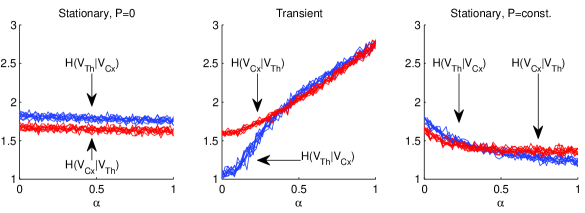
(b)

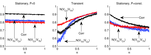
Figure 6: Nonlinear interdependence measures (a) $H$, (b) $N$ and maximum of absolute value of cross-correlation coefficients for varying coupling constants. Each measure is calculated for 10 independent realizations with different seeds. The parameter $\alpha$ scales the strength of connections from thalamus to cortex.

Consider first stationary signals with $P=0$ or $P=\mathrm{const}$. Without noise the system is in a fixed point and obviously it is impossible to obtain the connection strength. However, given the noise, in principle the dynamics in the neighborhood of the fixed point is also probed. Thus there is a possibility that the interdependence and the strength of the coupling could be established during stationary parts of the dynamics. It turns out that for null stimulation neither the interdependence measures nor the linear correlations detect any changes in the coupling strength (Figure 6, left column). For constant non-zero input there is a connection between the coupling strength and the values of the measure but they are anti-correlated and the dependence is not very pronounced (Figure 6, right column). One must also bear in mind that while it is possible to have no stimulation, in brain studies prolonged and constant stimulation in the present sense cannot be experimentally realized (at least for most sensory systems) because of the adaptation of receptors. The natural stimuli are necessarily transient.

To use the synchrony measures on the transient we cut out pieces of signal corresponding to the evoked potential, and pasted them one after another. Thus obtained pseudo-periodic signal contained the same underlying dynamics with each piece differing due to the noise. We then applied the same measures as we did for the stationary signals. In the simulations we calculated 50 “evoked potentials” (Figure 3) for each value of $\alpha$. Plots in the middle column of Figure 6 show the values of the synchronization measures evaluated for different coupling strengths. It can be seen that they are increasing functions of the coupling strength between the subsystems. Therefore, our approach is indeed a viable solution to the problem of data-based quantification of the coupling strength.

It is interesting to study the values of these interdependence measures in different cases. Observe that $H(V_{\text{Th}}|V_{\text{Cx}})>H(V_{\text{Cx}}|V_{\text{Th}})$ for $P=0$. The opposite is true for transients (for small $\alpha$). This is even more clearly visible for $N$. In all the cases linear correlations showed similar trends to the nonlinear measures $N(V_{\text{Th}}|V_{\text{Cx}}),N(V_{\text{Cx}}|V_{\text{Th}})$.

The asymmetry in the interdependence measures was originally intended to be used for inferring the direction of the coupling or driving. However, the inference of specific driving structure in every case must follow a careful analysis of underlying dynamics (see, for example, discussions in Quiroga et al. (2000) and Arnhold (1999)). Let us consider the plots in the middle column of Figure 6. For small $\alpha$ the dominant connections are from the cortex to the thalamus so one might expect that the state of the thalamus might be easier predictable from the states of the cortex than the other way round. Thus one would intuitively expect $H(V_{\text{Th}}|V_{\text{Cx}})>H(V_{\text{Cx}}|V_{\text{Th}})$. However, we observe the opposite. The reason is that the measures used are related to the relative number of degrees of freedom Arnhold (1999). Loosely speaking, as discussed Quiroga et al. (2000), the effective dimension of the driven system (thalamus for small $\alpha$) is usually higher than the dimension of the driver (which means that the response — the dynamics of the thalamus — is “more complex”). This effect is further enhanced by the fact that we stimulate the thalamus in moments unpredictable from the point of view of the cortex. Summarizing, the result is compatible with the analysis in Quiroga et al. (2000). What happens for higher $\alpha$ when the two measures become equal is probably the coupling between the two subsystems becoming so strong that the quality of prediction in any direction is comparable.

In the stationary case the situation is different as we observe the asymptotic behavior. It turns out that for $P=0$ for every $\alpha$, and for $P=\mathrm{const}>0$ for small $\alpha$ we have $H(V_{\text{Th}}|V_{\text{Cx}})>H(V_{\text{Cx}}|V_{\text{Th}})$. But it seems that another effect also plays a role here. The noise in the cortex has a higher amplitude than in the thalamus and as a consequence it is easier to predict the state of the thalamus from that of the cortex than in the other direction. The reason for this disparity in the amplitudes is the difference in the shape of the sigmoidal functions $\mathcal{S}_{q}$. To summarize, here, the asymmetry of the measures reflects internal properties of the two subsystems and not the symmetry properties of the coupling between them.

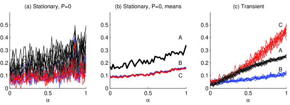
Figure 7: Nonlinear interdependence measures $H(\mathrm{X}_{1}|\mathrm{X}_{2})$, $H(\mathrm{X}_{2}|\mathrm{X}_{1})$ and maximum of absolute value of cross-correlation coefficients between signals from two symmetrically coupled Rössler-type systems with noise. Coupling strength is proportional to $\alpha$. The panels (a) and (c) present results of 10 simulations with different seeds. Additionally in stationary situation the means across repetitions are plotted for clarity in (b), the top curve (A) is cross-correlation. In stationary situation both nonlinear measures (B), (C) take similar values. On transients (c) $H(\mathrm{X}_{2}|\mathrm{X}_{1})$ (C) is higher than $H(\mathrm{X}_{1}|\mathrm{X}_{2})$ (B). The intermediate curves (A) are cross-correlation.

Figure 7 shows similar results obtained for two coupled Rössler-type systems. In stationary situation the interdependence measures are very noisy. Although a weak trend is visible, one would not be able to reliably discriminate between, say, $\alpha=0.25$ and $\alpha=0.75$. The equality of the measures in two directions is due to the fact that the systems are almost identical and symmetrically coupled.

If the interdependence is quantified on transient parts of the dynamics, the situation improves considerably. $H(\mathrm{X}_{2}|\mathrm{X}_{1})$ has a high slope and is a very good measure of the coupling strength between the systems. Although $H(\mathrm{X}_{1}|\mathrm{X}_{2})$ has a slope comparable to that in the stationary case for $P=0$, the variability of the results is much smaller, compared to the size of the fluctuation in the ensemble mean in the stationary case. The difference between $H(\mathrm{X}_{2}|\mathrm{X}_{1})$ and $H(\mathrm{X}_{1}|\mathrm{X}_{2})$ reflects the asymmetry of the driving (which makes the dynamics of $\mathrm{X}_{1}$ “more complex” than the dynamics of $\mathrm{X}_{2}$), not of the coupling (which is symmetric).

IV.2 Influence of noise

The performance of the procedure described above depends on the level of noise present in the system. To study this dependence we performed the simulations of the thalamocortical model (the case of transient dynamics) for 25%, 50%, 100% and 200% of the original noise level. We found that for increasing level of noise the dynamics of the system may change qualitatively: if the noise level is large enough the system may be kicked out of the basin of attraction of the fixed point and would not return there after $P$ is reset to $0$. Instead it may fall into the basin of attraction of another stable orbit or switch between the basins repeatedly. We observed such behavior only once for 2500 simulations performed with 200% of the original noise and this trial was excluded from the analysis. Such behavior becomes more frequent with increasing noise (e.g. 400%) and so we did not study this situation as it was very different from the original dynamics of the system.

As one would expect, the higher the noise, the less sensitive the measures are (Fig. 8). However, even for twice the original level of noise a weak trend in the interdependence is clearly visible.

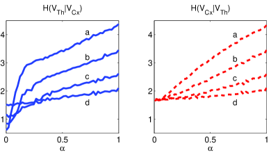
Figure 8: Nonlinear interdependence $H$ in thalamocortical loop model for varying level of noise. The curves represent the values of the measure on transients. Noise level are 25% (a), 50% (b), 100% (c) and 200% (d) of the original noise.

IV.3 Time-resolved measure $H_{i}$

Since we are interested in the dynamics of non-autonomous systems one might wonder if time-resolved measures, such as $H_{i}$ introduced in Andrzejak et al. (2006), would not perform better in the problem of inferring connection strength. We performed tests on cut-and-pasted transient signals. This problem is different from the one studied in Andrzejak et al. (2006).

(a)

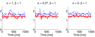
(b)

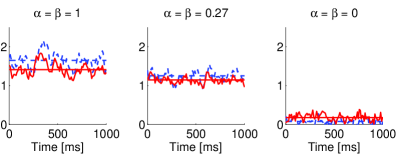
Figure 9: Time-resolved nonlinear interdependence measure $H_{i}(V_{\text{Th}}|V_{\text{Cx}})$ (dashed lines) and $H_{i}(V_{\text{Cx}}|V_{\text{Th}})$ (solid lines) for 3 different values of the coupling $\alpha$. The means are shown with horizontal lines. (a) $\beta=1$, (b) $\beta=\alpha$.

There, two Lorenz systems were coupled for short periods of time and $H_{i}$ was shown to identify these times of coupling well. In our problem the coupling is constant in time, it is only the input to the system that is varying. For the problem at hand the values of $H_{i}$ do not seem to change with varying coupling constant $\alpha$ (Fig. 9, (a)) when $\beta$ is constant, $\beta=1$. The reason for this may be that even for $\alpha=0$ the subsystems are coupled through the connections from cortex to thalamus. This hypothesis can be tested in another experiment, where all the connections between the subsystems are scaled and $\alpha=\beta$.

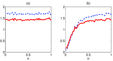
Figure 10: Mean value of the time-resolved interdependence measure $H_{i}(V_{\text{Th}}|V_{\text{Cx}})$ (dashed lines) and $H_{i}(V_{\text{Cx}}|V_{\text{Th}})$ (solid lines). (a) $\beta=1$, (b) $\beta=\alpha$

Indeed, in this setup the measure $H_{i}$ is sensitive to the coupling strength (Fig. 9, (b); Fig. 10).

One may also note that $H_{i}(V_{\text{Th}}|V_{\text{Cx}})$ is on average higher than $H_{i}(V_{\text{Cx}}|V_{\text{Th}})$, exactly as for $H$ in case of $P=0$ and contrary to what is observed using $H$ on transients (Fig. 6 (a)). Thus it seems that for the problem of inferring coupling strength between two systems the optimal approach is to use $H$ or $N$, or linear correlations, on the transients, as described in Section IV.1.

V Conclusions

To summarize, we have proposed a general approach for inference of the coupling strength using transient parts of dynamics. We have shown that our approach gives more information about the coupling between subsystems than the approach using the stationary part of dynamics in case when the asymptotic dynamics is on a fixed point. We have checked the validity of this approach on a model of a thalamocortical loop of sensory systems and on two coupled Rössler-type oscillators. We showed that our method is quite robust with respect to increasing level of noise as long as the dynamics does not change qualitatively. We have also shown that this method measures different aspects of coupling than a time-resolved measure $H_{i}$ and than linear correlations. We believe that our approach will be of use in many other physical systems studied in the stimulus-response paradigm, especially in the experimental context.

The results of Section IV.1 are compatible with our preliminary studies of data from real neurophysiological experiments Świejkowski (2007). There one cannot discern coupling strength in two contextual situations basing on stationary recordings, but the analysis of transients leads to clear differences between two variants of experiment. The results of this analysis will be published elsewhere.

*

Appendix A Parameters of the models

We use the following equations for the model of thalamocortical loop:

$$\tau\frac{\mathrm{d}E_{\text{Th}}}{\mathrm{d}t} = -E_{\text{Th}}+(k_{E_{\text{Th}}}-r{E_{\text{Th}}})$$

$$\times\mathcal{S}_{E_{\text{Th}}}(P-c_{1}I_{\text{Th}}+\beta e_{1}E_{\text{Cx}}+\xi_{1}),$$

$$\tau\frac{\mathrm{d}I_{\text{Th}}}{\mathrm{d}t} = -I_{Th}+(k_{I_{\text{Th}}}-r{I_{\text{Th}}})$$

$$\times\mathcal{S}_{I_{Th}}(Q+c_{2}{E_{\text{Th}}+\beta e_{2}E_{\text{Cx}}}+\xi_{2}),$$

$$\tau\frac{\mathrm{d}E_{\text{Cx}}}{\mathrm{d}t} = -E_{Cx}+(k_{E_{\text{Cx}}}-rE_{\text{Cx}})$$

$$\times\mathcal{S}_{E_{\text{Cx}}}(c_{3}E_{\text{Cx}}-c_{4}I_{\text{Cx}}+\alpha e_{3}E_{\text{Th}}+\xi_{3}),$$

$$\tau\frac{\mathrm{d}I_{\text{Cx}}}{\mathrm{d}t} = -I_{\text{Cx}}+(k_{I_{\text{Cx}}}-r{I_{\text{Cx}}})$$

$$\times\mathcal{S}_{I_{\text{Cx}}}(c_{5}E_{\text{Cx}}-c_{6}{I_{\text{Cx}}}+\alpha e_{4}E_{\text{Th}}+\xi_{4}),$$

where

$$\mathcal{S}_{q}(x)=\frac{1}{1+e^{-a_{q}(x-\vartheta_{q})}}-\frac{1}{1+e^{a_{q}\vartheta_{q}}},$$

$q$ standing for $E_{\text{Th}},I_{\text{Th}},E_{\text{Cx}},I_{\text{Cx}},$ and $\xi_{i}$, $i=1\ldots 4$ are noise inputs. The normalizing constants $k_{q}$ are defined as $k_{q}=1-\frac{1}{1+e^{a_{q}\vartheta_{q}}}$.

In the numerical experiments we used the following parameter values:

$$c_{1} =1.35 c_{2} =5.35 c_{3} =15$$

$$c_{4} =15 c_{5} =15 c_{6} =3$$

$$e_{1} =10 e_{2} =20 e_{3} =10$$

$$e_{4} =5 \tau =10\mathrm{ms} r =1$$

$$a_{E_{\text{Th}}} =0.55 \vartheta_{E_{\text{Th}}} =11 a_{I_{\text{Th}}} =0.25$$

$$\vartheta_{I_{\text{Th}}} =9 a_{E_{\text{Cx}}} =1 \vartheta_{E_{\text{Cx}}} =2$$

$$a_{I_{\text{Cx}}} =2 \vartheta_{I_{\text{Cx}}} =2.5$$

The strength of connections was scaled by $\alpha\in[0,1]$. Everywhere except in Section IV.3 we used $\beta=1$. In Section IV.3 we used either $\alpha\in[0,1]$ and $\beta=1$, or $\alpha\in[0,1]$ and $\beta=\alpha$.

References

- Pikovsky et al. (2001) A. Pikovsky, M. Rosenblum, and J. Kurths, Synchronization. A universal concept in nonlinear sciences (Cambridge Univ. Press, 2001).
- Pecora and Carroll (1990) L. M. Pecora and T. L. Carroll, Phys. Rev. Lett. 64, 821 (1990).
- Rosenblum et al. (1996) M. G. Rosenblum, A. S. Pikovsky, and J. Kurths, Phys. Rev. Lett. 76, 1804 (1996).
- Rulkov et al. (1995) N. F. Rulkov, M. M. Sushchik, L. S. Tsimring, and H. D. I. Abarbanel, Phys. Rev. E 51, 980 (1995).
- Pecora et al. (1995) L. M. Pecora, T. L. Carroll, and J. F. Heagy, Phys. Rev. E 52, 3420 (1995).
- Kocarev and Parlitz (1996) L. Kocarev and U. Parlitz, Phys. Rev. Lett. 76, 1816 (1996).
- Schiff et al. (1996) S. J. Schiff, P. So, T. Chang, R. E. Burke, and T. Sauer, Phys. Rev. E 54, 6708 (1996).
- Wójcik et al. (2001) D. Wójcik, A. Nowak, and M. Kuś, Phys. Rev. E 63, 36221 (2001).
- Rosenblum et al. (2001) M. Rosenblum, A. Pikovsky, J. Kürths, C. Schäfer, and P. A. Tass, in Handbook of Biological Physics, vol. 4 edited by F. Moss and S. Gielen (Elsevier, 2001), p. 279.
- Singer and Gray (1995) W. Singer and C. M. Gray, Ann. Rev. Neurosci. 18, 555 (1995).
- Varela et al. (2001) F. Varela, J. P. Lachaux, E. Rodriguez, and J. Martinerie, Nat. Rev. Neurosci. 2, 229 (2001).
- Arnhold (1999) J. Arnhold, Physica D 134, 419 (1999).
- Kamiński et al. (2001) M. Kamiński, M. Ding, W. A. Truccolo, and S. L. Bressler, Biol. Cybern. 85, 145 (2001).
- Quiroga et al. (2002) R. Quian Quiroga, A. Kraskov, T. Kreuz, and P. Grassberger, Phys. Rev. E 65, 041903 (2002).
- Niebur et al. (2002) E. Niebur, S. S. Hsiao, and K. O. Johnson, Curr. Opin. Neurobiol. 12, 190 (2002).
- Angelini et al. (2004) L. Angelini, M. D. Tommaso, M. Guido, K. Hu, P. C. Ivanov, D. Marinazzo, G. Nardulli, L. Nitti, M. Pellicoro, C. Pierro, et al., Phys. Rev. Lett. 93, 038103 (2004).
- Lai et al. (2007) Y. C. Lai, M. G. Frei, I. Osorio, and L. Huang, Phys. Rev. Lett. 98, 108102 (2007).
- Korzeniewska et al. (2007) A. Korzeniewska, C. M. Crainiceanu, R. Kuś, P. J. Franaszczuk, and N. E. Crone, Hum. Brain Mapp. (2007).
- Fell et al. (2001) J. Fell, P. Klaver, K. Lehnertz, T. Grunwald, C. Schaller, C. E. Elger, and G. Fernández, Nat. Neurosci. 4, 1259 (2001).
- Kramer et al. (2004) M. A. Kramer, E. Edwards, M. Soltani, M. S. Berger, R. T. Knight, and A. J. Szeri, Phys. Rev. E 70, 011914 (2004).
- Kublik et al. (2003) E. Kublik, D. A. Świejkowski, and A. Wróbel, Acta Neurobiol. Exp. (Wars) 63, 377 (2003).
- Kublik (2004) E. Kublik, Acta Neurobiol. Exp. (Wars) 64, 229 (2004).
- Świejkowski (2007) D. Świejkowski, Ph.D. thesis, Nencki Institute of Experimental Biology (2007).
- Wróbel et al. (2007) A. Wróbel, A. Ghazaryan, M. Bekisz, W. Bogdan, and J. Kamiński, J. Neurosci. 27, 2230 (2007).
- Łęski et al. (2007) S. Łęski, D. K. Wójcik, J. Tereszczuk, D. A. Świejkowski, E. Kublik, and A. Wróbel, Neuroinformatics 5, 207 (2007).
- Andrzejak et al. (2006) R. G. Andrzejak, A. Ledberg, and G. Deco, New Journal of Physics 8, 6 (2006).
- Jánosi and Tél (1994) Jánosi and Tél, Phys. Rev. E 49, 2756 (1994).
- Wilson and Cowan (1972) H. R. Wilson and J. D. Cowan, Biophys. J. 12, 1 (1972).
- Wilson and Cowan (1973) H. R. Wilson and J. D. Cowan, Kybernetik 13, 55 (1973).
- Shepherd (2004) G. M. Shepherd, ed., The Synaptic organization of the brain (Oxford Univ. Press, 2004), 5th ed.
- Quiroga et al. (2000) R. Q. Quiroga, J. Arnhold, and P. Grassberger, Phys. Rev. E 61, 5142 (2000).
- Takens (1980) F. Takens, in Dynamical Systems and Turbulence (Warwick 1980), edited by D. A. Rand and L.-S. Young (Springer-Verlag, Berlin, 1980), vol. 898 of Lecture Notes in Mathematics , pp. 366–381.
- Andrzejak et al. (2003) R. G. Andrzejak, A. Kraskov, H. Stögbauer, F. Mormann, and T. Kreuz, Phys. Rev. E 68, 066202 (2003).
- Theiler (1986) J. Theiler, Phys. Rev. A 34, 2427 (1986).
- Kantz and Schreiber (2004) H. Kantz and T. Schreiber, Nonlinear Time Series Analysis (Cambridge Univ. Press, Cambridge, UK, 2004).
- Letellier and Rössler (2006) C. Letellier and O. E. Rössler, Scholarpedia (2006), 1(10):1721, URL www.scholarpedia.org/article/Rossler_attractor.