Cascaded Orthogonal Space-Time Block Codes for Wireless Multi-Hop Relay Networks

Abstract

Distributed space-time block coding is a diversity technique to mitigate the effects of fading in multi-hop wireless networks, where multiple relay stages are used by a source to communicate with its destination. This paper proposes a new distributed space-time block code called the cascaded orthogonal space-time block code (COSTBC) for the case where the source and destination are equipped with multiple antennas and each relay stage has one or more single antenna relays. Each relay stage is assumed to have receive channel state information (CSI) for all the channels from the source to itself, while the destination is assumed to have receive CSI for all the channels. To construct the COSTBC, multiple orthogonal space-time block codes are used in cascade by the source and each relay stage. In the COSTBC, each relay stage separates the constellation symbols of the orthogonal space-time block code sent by the preceding relay stage using its CSI, and then transmits another orthogonal space-time block code to the next relay stage. COSTBCs are shown to achieve the maximum diversity gain in a multi-hop wireless network with flat Rayleigh fading channels. Several explicit constructions of COSTBCs are also provided for two-hop wireless networks with two and four source antennas and relay nodes. It is also shown that COSTBCs require minimum decoding complexity thanks to the connection to orthogonal space-time block codes.

I Introduction

It is well known that for point-to-point multiple antenna wireless channels, space-time block codes (STBCs) [1, 2] improve the bit error rate performance by introducing redundancy across multiple antennas and time. Through special designs, STBCs increase the diversity gain, defined as the negative of the exponent of the signal-to-noise ratio (SNR) in the pairwise error probability expression at high SNR [2]. Recently, the concept of STBC has been extended to wireless networks, where the antennas of other nodes in the network (called relays) are used to construct STBC in a distributed manner to improve the diversity gain between a particular source and its destination [3, 4, 5, 6, 7, 8, 9, 10].

Prior work on DSTBC [3, 5, 6, 7, 8] considers a two-hop wireless network, where in the first hop the source transmits the signal to all the relays and in the next hop, all relays simultaneously transmit a function of the received signal to the destination. If a decode and forward (DF) strategy is used, each relay decodes the incoming signal from the source and then transmits a vector or a matrix depending on whether it has one or more than one antenna [4, 3, 11]. The matrix obtained by stacking all the vectors or matrices transmitted by the relays is called a DSTBC. Since each relay decodes the received signal, the criteria for designing a DSTBC with DF is same as the criteria for designing STBCs in point-to-point channels [2]. Due to independent decoding at each relay, however, the diversity gain of DSTBC with DF is limited by the minimum of the diversity gains between the source and all the different relays.

If an amplify and forward (AF) strategy is used, each relay is only allowed to transmit a function of the received signal without any decoding, subject to its power constraint. A DSTBC design is proposed in [5, 7] using an AF strategy, where each relay transmits a relay specific unitary transformation of the received signal. This DSTBC construction, however, is limited to two-hop wireless networks where each relay is equipped with a single antenna. It was shown in [5, 7], that to maximize the diversity gain, the DSTBC transmitted by all relays using a unitary transformation should be a full-rank STBC. Algebraic constructions of maximum diversity gain achieving DSTBC for the two-hop wireless network are provided in [12, 13, 14, 15].

Recently, there has been growing interest in multi-hop wireless networks, where more than two hops are required for a source signal to reach its destination. Consequently, there is a strong case to construct DSTBCs that can achieve maximum diversity gain in a large wireless networks with multiple hops. Unfortunately, most prior work on constructing DSTBC for maximizing the diversity gain only considers a two-hop wireless network [4, 3, 11, 5, 7] and does not readily extends to more than two-hops.

In this paper we design maximum diversity gain achieving DSTBC’s for multi-hop wireless networks. We assume that the source and the destination terminals have multiple antennas while the relays in each stage have a single antenna. We also assume that all the nodes in the network (source, relays and destination) can only work in half-duplex mode (cannot transmit and receive at the same time) and each relay and the destination has perfect receive channel state information (CSI).

We propose an AF based multi-hop DSTBC, called the cascaded orthogonal space-time block code (COSTBC), where an orthogonal space-time code (OSTBC) [16] is used by the source and each relay stage to communicate with its adjacent relay stage. OSTBCs are considered because of their single symbol decodable property [1, 16], i.e. each constellation symbol of the OSTBC can be separated at the receiver with independent noise terms. To construct COSTBCs the single symbol decodable property of OSTBC is used by each relay stage to separate the constellation symbols of the OSTBC transmitted by the preceding stage and transmit another OSTBC to the next relay stage.

With our proposed COSTBC design, in the first time slot the source transmits an OSTBC to the first relay stage. Using the single symbol decodable property of the OSTBC, each relay of the first relay stage separates the different OSTBC constellation symbols from the received signal and transmits a codeword vector in the next time slot, such that the matrix obtained by stacking all the codeword vectors transmitted by the different relays of the first relay stage is an OSTBC. These operations are repeated by subsequent relay stages. It is worth noting that with COSTBC, no signal is decoded at any of the relays, therefore COSTBC construction with single antenna relays is equivalent to COSTBC construction with multiple antenna relays. Thus without loss of generality in this paper we only consider COSTBC construction for single antenna relays. The diversity gain analysis presented in this paper for COSTBC, however, is very general and applies to the multiple antenna relay case as well.

We prove that the COSTBCs achieve the maximum diversity gain in two or more hop wireless networks when CSI is available at each relay and the destination in the receive mode. We first show this for a two-hop wireless network and then using mathematical induction generalize it to the multi-hop case. We also give an explicit construction of COSTBCs for different source antennas and relay configurations. We prove that the COSTBCs have the single symbol decodable property similar to OSTBCs. We also show that cascading multiple OSTBCs to construct COSTBC preserves the single symbol decodable property of OSTBCs and as a result COSTBCs require minimum decoding complexity.

During the preparation of this manuscript we came across three related papers on DSTBC construction for multi-hop wireless networks [17, 18, 19] . We briefly review this work and compare them with the proposed COSTBCs.

Maximum diversity gain achieving DSTBCs are constructed in [17] for single antenna multi-hop wireless network, where each node (the source, each relay and the destination) has single antenna, by extending the AF strategy with unitary transformation for two-hop wireless networks [5]. It can be shown, however, that the AF strategy with unitary transformation to construct DSTBC does not extend easily to multi-hop wireless networks with multiple source or destination antennas. Thus, COSTBC is a more general solution than the one proposed in [17]. Moreover, to achieve the maximum diversity gain with the strategy proposed in [17], the coding block length, the time across which coding needs to be done, is proportional to the product of the number of relay nodes, whereas with COSTBC it is proportional to the number of relay nodes. This makes COSTBC more suited for low-latency applications, e.g. voice communication.

The focus of [18, 19] is on the construction of DSTBCs that can achieve the optimal diversity multiplexing (DM) tradeoff [20] in a multi-hop wireless network. In [18] a full-duplex multi-hop wireless network (each node can transmit and receive at the same time) is considered, whereas [19] mainly considers a half duplex multi-hop wireless network. In [18] a parallel AF strategy is proposed which divides the total number of paths from the source to the destination into non-overlapping groups and transmits an STBC with non-vanishing determinant property [21] through each group simultaneously. It is shown that this strategy achieves the maximum diversity gain and maximum multiplexing gain points of the optimal DM-tradeoff in a multi-hop wireless network for some special cases. An AF strategy similar to delay diversity strategy of [2] is proposed in [19] to achieve the DM-tradeoff for the half-duplex multi-hop wireless network where both the source and the destination are equipped with single antenna. In comparison to the strategies of [18, 19], COSTBC only achieves the maximum diversity gain and not the maximum multiplexing gain. Due to the use of OSTBCs, however, the decoding complexity of COSTBC is significantly less than the strategies of [18, 19] where STBCs with high decoding complexity are used. Thus COSTBCs are more suited for practical implementation than the strategies of [18, 19].

Notation: Let ${{\mathbf{A}}}$ denote a matrix, ${\bf a}$ a vector and $a_{i}$ the $i^{th}$ element of ${\bf a}$. The $i^{th}$ eigenvalue of ${\mathbf{A}}$ is denoted by $\lambda_{i}({\mathbf{A}})$ and the maximum and minimum eigenvalue of ${\mathbf{A}}$ by $\lambda_{max}({\mathbf{A}})$ and $\lambda_{min}({\mathbf{A}})$, respectively, if the eigenvalues of ${\mathbf{A}}$ are real. The determinant and trace of matrix ${\bf A}$ are denoted by $\det({{\mathbf{A}}})$ and ${\it{tr}}({{\mathbf{A}}})$, while ${\mathbf{A}}^{\frac{1}{2}}$ denotes the element wise square root of matrix ${\bf A}$ with all non-negative entries. The field of real and complex numbers is denoted by ${\mathbb{R}}$ and ${\mathbb{C}}$, respectively. The space of $M\times N$ matrices with complex entries is denoted by ${{\mathbb{C}}}^{M\times N}$. The Euclidean norm of a vector $\bf a$ is denoted by $|{\mathbf{a}}|$. An $m\times m$ identity matrix is denoted by ${\bf I}_{m}$ and ${\bf 0}_{m}$ is as an all zero $m\times m$ matrix. The superscripts ${}^{T},^{*},^{{\dagger}}$ represent the transpose, transpose conjugate and element wise conjugate. For matrices ${\mathbf{A}},{\mathbf{B}}$ by ${\mathbf{A}}\leq{\mathbf{B}},{\mathbf{A}},{\mathbf{B}}\in{{\mathbb{C}}}^{m\times m}$ we mean ${\mathbf{x}}{\mathbf{A}}{\mathbf{x}}^{*}\leq{\mathbf{x}}{\mathbf{B}}{\mathbf{x}}^{*},\ \forall{\mathbf{x}}\in{{\mathbb{C}}}^{1\times m}$. The expectation of function $f(x)$ with respect to $x$ is denoted by ${{\mathbb{E}}}_{\{x\}}f(x)$. The maximum and minimum value of the set $\{a_{1},a_{2},\ldots,a_{m}\}$ where $a_{i}\in{\mathbb{R}},\ i=1,2,\ldots,m$ are denoted by $\max\{a_{1},a_{2},\ldots,a_{m}\}$ and $\min\{a_{1},a_{2},\ldots,a_{m}\}$. A circularly symmetric complex Gaussian random variable $x$ with zero mean and variance $\sigma^{2}$ is denoted as $x\sim{\cal CN}(0,\sigma)$. We use the symbol $\stackrel{{\scriptstyle.}}{{=}}$ to represent exponential equality i.e., let $f(x)$ be a function of $x$, then $f(x)\stackrel{{\scriptstyle.}}{{=}}x^{a}$ if $\lim_{x\rightarrow\infty}\frac{\log(f(x))}{\log x}=a$ and similarly $\stackrel{{\scriptstyle.}}{{\leq}}$ and $\stackrel{{\scriptstyle.}}{{\geq}}$ denote the exponential less than or equal to and greater than or equal to relation, respectively. To define a variable we use the symbol $:=$.

Organization: The rest of the paper is organized as follows. In Section II, we describe the system model for the multi-hop wireless network and review the key assumptions. In Section III, COSTBC construction is described. A diversity gain analysis of COSTBCs is presented in Section IV for the $2$-hop case and generalized to $N$-hop network case in Section V. In Section VI, explicit constructions of COSTBCs are provided which achieve maximum diversity gain for different number of source antenna and relay node configurations. Some numerical results are provided in Section VII. Final conclusions are made in Section VIII.

II System Model

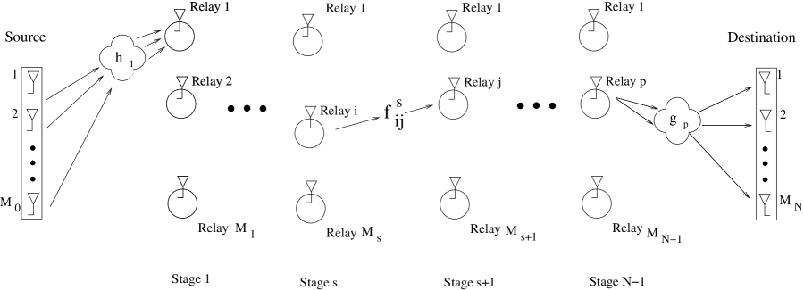
Figure 1: System Block Diagram of a N-hop Wireless Network

We consider a multi-hop wireless network where a source terminal with $M_{0}$ antennas wants to communicate with a destination terminal with $M_{N}$ antennas via $N-1$ relay stages as shown in Fig. 1. Each relay in any relay stage has a single antenna; $M_{n}$ denotes the number of relays in the $n^{th}$ relay stage. It is assumed that the relays do not generate their own data and only operate in half-duplex mode. A half-duplex assumption is made since full-duplex nodes are difficult to realize in practice. Similar to the model considered in [18], we assume that any relay of relay stage $n$ can only receive the signal from any relay of relay stage $n-1$, i.e. we consider a directed multi-hop wireless network. In a practical system this assumption can be realized by allowing every third relay stage to be active (transmit or receive) at the same time. To keep the relay functionality and relaying strategy simple we do not allow relay nodes to cooperate among themselves. We assume that there is no direct path between the source and the destination. This is a reasonable assumption for the case when relay stages are used for coverage improvement and the signal strength on the direct path is very weak. Throughout this paper we refer to this multi-hop wireless network with $N-1$ relay stages as an $N$-hop network.

As shown in Fig. 1, the channel between the source and the $i^{th}$ relay of the first stage of relays is denoted by ${\mathbf{h}}_{i}=[h_{1i}\ h_{2i}\ \ldots\ h_{M_{0}i}]^{T},\ i=1,2,\ldots,M_{1}$, between the $j^{th}$ relay of relay stage $s$ and the $k^{th}$ relay of relay stage $s+1$ by $f^{s}_{jk},\ s=0,1,\ldots,N-2,\ j=1,2,\ldots,M_{s},\ k=1,2,\ldots,M_{s+1}$ and the channel between the relay stage $N-1$ and the $\ell^{th}$ antenna of the destination by ${\mathbf{g}}_{\ell}=[g_{1\ell}\ g_{2\ell}\ \ldots\ g_{M_{N-1}\ell}]^{T},\ \ell=1,2,\ldots,M_{N}$. We assume that ${\mathbf{h}}_{i}\in{\mathbb{C}}^{M_{0}\times 1}$, $f^{s}_{jk}\in{\mathbb{C}}^{1\times 1}$, ${\mathbf{g}}_{l}\in{\mathbb{C}}^{M_{N-1}\times 1}$ with independent and identically distributed (i.i.d.) ${\cal CN}(0,1)$ entries for all $i,j,k,\ell,s$. We assume that the $m^{th}$ relay of $n^{th}$ stage knows ${\mathbf{h}}_{i},f^{s}_{jk},\ \forall\ i,\ j,\ k,s=1,2,\ldots,n-2,\ f^{n-1}_{jm}\ \forall j$ and the destination knows ${\mathbf{h}}_{i},f^{s}_{jk},{\mathbf{g}}_{l},\ \forall\ i,j,k,l,s$. We further assume that all these channels are frequency flat and block fading, where the channel coefficients remain constant in a block of time duration $T_{c}$ and change independently from block to block. We assume that the $T_{c}$ is at least $\max\{M_{0},M_{1},\ldots,M_{N-1}\}$.

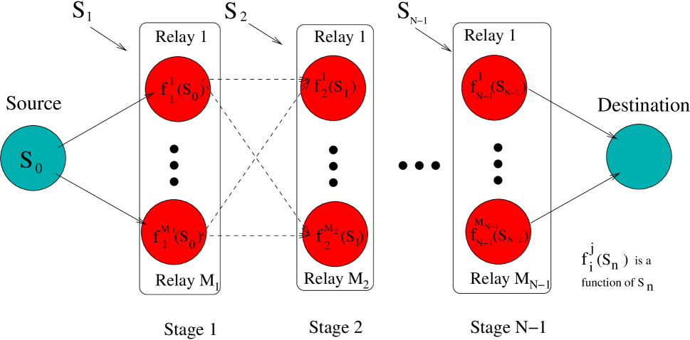
Figure 2: An Illustration Of The DSTBC Design Problem

II-A Problem Formulation

Definition 1

(STBC) [22] A rate-$L/T$ $T\times{N_{t}}$ design ${{\mathbf{D}}}$ is a $T\times{N_{t}}$ matrix with entries that are complex linear combinations of $L$ complex variables $s_{1},s_{2},\ldots,s_{L}$ and their complex conjugates. A rate-$L/T$ $T\times{N_{t}}$ STBC ${\bf S}$ is a set of $T\times{N_{t}}$ matrices that are obtained by allowing the $L$ variables $s_{1},s_{2},\ldots,s_{L}$ of the rate-$L/T$ $T\times{N_{t}}$ design ${\mathbf{D}}$ to take values from a finite subset ${{\mathbb{C}}}^{f}$ of the complex field ${{\mathbb{C}}}$. The cardinality of ${\bf S}=|{{\mathbb{C}}}^{f}|^{L}$, where $|{{\mathbb{C}}}^{f}|$ is the cardinality of ${\mathcal{C}}$. We refer to $s_{1},s_{2},\ldots,s_{L}$ as the constituent symbols of the STBC.

Definition 2

A DSTBC ${\cal C}$ for a $N$-hop network is a collection of codes $\left\{{\mathbf{S}}_{0},{\mathbf{S}}_{1},\ldots,{\mathbf{S}}_{N-1}\right\}$, where ${\mathbf{S}}_{0}$ is the STBC transmitted by the source and ${\mathbf{S}}_{n}=[{\bf f}^{1}_{n}({{\mathbf{S}}_{n-1}})\ldots{\bf f}^{M_{n}}_{n}({{\mathbf{S}}_{n-1}})]$ is the STBC transmitted by relay stage $n$, where ${\bf f}^{j}_{n}({{\mathbf{S}}_{n-1}})$ is the vector transmitted by the $j^{th}$ relay of stage $n$ which is a function of ${{\mathbf{S}}_{n-1}},\ j=0,\ldots,M_{n},n=1,\ldots,N-1$. An example of a DSTBC is illustrated in Fig. 2.

Definition 3

The diversity gain [2, 5] of a DSTBC ${\cal C}$ is defined as

$$d_{\cal C}=-\lim_{E\rightarrow\infty}\frac{\log{P_{e}\left(E\right)}}{\log{E}},$$

$P_{e}\left(E\right)$ is the pairwise error probability (PEP) using coding strategy ${\cal C}$, and $E$ is the sum of the transmit power used by each node in the network.

The problem we consider is in this paper is to design DSTBCs that achieve the maximum diversity gain in a $N$-hop network. To identify the limits on the maximum possible diversity gain in a $N$-hop network, an upper bound on the diversity gain achievable with any DSTBC is presented next.

Theorem 1

The diversity gain $d_{\cal C}$ of DSTBC ${\cal C}$ for an $N$-hop network is upper bounded by

$$\min\left\{M_{n}M_{n+1}\right\}\ \ n=0,1,\ldots,N-1.$$

Proof: Let $d_{\cal C}$ be the diversity gain of coding strategy ${\cal C}$ for an $N$-hop network. Let $d_{n}$ be the diversity gain of the best possible DSTBC ${\cal C}^{opt}$ that can be used between relay stage $n$ and $n+1$ when all the relays in relay stage $n$ and relay stage $n+1$ are allowed to collaborate, respectively, and the source message is known to all the relays of relay stage $n$ without any error and all the relays of the relay stage $n+1$ can send the received signal to the destination error free. Then, clearly, $d_{\cal C}\leq d_{n}$. Since the channel between the relay stage $n$ and $n+1$ is a multiple antenna channel with $M_{n}$ transmit and $M_{n+1}$ receive antennas, $d_{n}\leq M_{n}M_{n+1}$. Hence $d_{\cal C}\leq M_{n}M_{n+1}$. Since this is true for every $n=0,1,\ldots,N-1$, it follows that $d_{\cal C}\leq\min\{M_{n}M_{n+1}\},\ n=0,1,\ldots,N-1$.  ∎

Thus, Theorem 1 implies that the maximum diversity gain achievable in a $N$-hop network is equal to the minimum of the maximum diversity gain achievable between any two relay stages, when all the relays in each relay stage are allowed to collaborate. In our system model we do not allow any cooperation between relays, and hence designing a DSTBC that achieves the diversity gain upper bound without any cooperation is difficult.

For the case of $2$-hop networks, DSTBCs have been proposed to achieve the maximum diversity gain [5, 7]. It is worth noting that designing DSTBCs that achieve the maximum diversity gain in a $N$-hop network is a difficult problem. The difficulty is two-fold: proposing a “good” DSTBC and analyzing its diversity gain. In the next section we describe our novel COSTBC construction and prove that it achieves the maximum diversity gain in a $N$-hop network. As it will be clear in the next section, using OSTBCs to construct COSTBC simplifies the diversity gain analysis, significantly.

III Cascaded Orthogonal Space-Time Code

In this section we introduce the COSTBC design for a $N$-hop network. Before introducing COSTBC we need the following definitions.

Definition 4

With $T\geq{N_{t}}$, a rate $L/T$ $T\times{N_{t}}$ STBC ${\bf S}$ is called full-rank or fully-diverse or is said to achieve maximum diversity gain if the difference of any two matrices ${\mathbf{M}}_{1},{\mathbf{M}}_{2}\in{\bf S}$ is full-rank,

$$\min_{{\mathbf{M}}_{1}\neq{\mathbf{M}}_{2},\ {\mathbf{M}}_{1},{\mathbf{M}}_{2}\in{\bf S}}rank({\mathbf{M}}_{1}-{\mathbf{M}}_{2})={N_{t}}.$$

Definition 5

(OSTBC) A rate-$L/K$ $K\times K$ STBC ${\bf S}$ is called an orthogonal space-time block code (OSTBC) if the design ${\mathbf{D}}$ from which it is derived is orthogonal i.e. ${{\mathbf{D}}}{{\mathbf{D}}}^{*}=(|s_{1}|^{2}+\ldots+|s_{L}|^{2}){\bf I}_{K}$.

Definition 6

Let ${\bf S}$ be a rate-$L/K$ $K\times K$ STBC. Then, using CSI, if each of the constituent symbols $s_{i},\ i=1,\ldots,L$ of ${\bf S}$ can be separated/decoded independently of $s_{j}$ $\forall i\neq j\ i,j=1,\ldots,L$ with independent noise terms, then ${\bf S}$ is called a single symbol decodable STBC.

Remark 1

OSTBCs are single symbol decodable STBCs [16].

With these definitions we are now ready to describe COSTBC for a $N$-hop network.

COSTBC is a DSTBC where each ${\mathbf{S}}_{n},\ n=0,1,\ldots,N-1$ is an OSTBC. Thus, with COSTBC the source transmits a rate-$L/M_{0}$ $M_{0}\times M_{0}$ OSTBC ${\mathbf{S}}_{0}$ in time slot of duration $M_{0}$. How to construct OSTBCs ${\mathbf{S}}_{n},n=1,\ldots,N-1$ is detailed in the following. Let ${\mathbf{S}}_{0}$ be a rate-$L/M_{0}$ $M_{0}\times M_{0}$ OSTBC transmitted by the source OSTBC ${\bf S}_{0}\in{\mathbb{C}}^{M_{0}\times M_{0}}$ to all the relays of relay stage $1$. Then the received signal ${\mathbf{r}}_{k}^{1}\in{\mathbb{C}}^{M_{0}\times 1}$ at relay $k$ of relay stage $1$ can be written as

$${\mathbf{r}}_{k}^{1}=\sqrt{E_{0}}{\mathbf{S}}_{0}{\mathbf{h}}_{k}+{\mathbf{n}}_{k}^{1}$$ (1)

where ${{\mathbb{E}}}tr({\mathbf{S}}_{0}^{*}{\mathbf{S}}_{0})=M_{0}$ and $E_{0}$ is the power transmitted by the source at each time instant. The noise ${\mathbf{n}}_{k}^{1}$ is the $M_{0}\times 1$ spatio-temporal white complex Gaussian noise independent across relays with ${\mathbb{E}}{\mathbf{n}}_{k}^{1}{\mathbf{n}}_{k}^{1*}={\bf I}_{M_{0}}$. Since ${\bf S}_{0}$ is an OSTBC, using CSI, the received signal ${\mathbf{r}}_{k}^{1}$ can be transformed into ${\tilde{\mathbf{r}}}^{1}_{k}\in{\mathbb{C}}^{L\times 1}$, where

$${\tilde{\mathbf{r}}}_{k}^{1}=\sqrt{E_{0}}\underbrace{\left[\begin{array}[]{cccc}\sum_{m=1}^{M_{0}}|h_{mk}|^{2}&0&0\\ 0&\ddots&0\\ 0&0&\sum_{m=1}^{M_{0}}|h_{mk}|^{2}\\ \end{array}\right]}_{\mathsf{H}}{\mathbf{s}}+{\tilde{\mathbf{n}}}_{k}^{1}$$ (2)

and ${\mathbf{s}}=[s_{1},s_{2},\ \ldots,\ s_{L}]^{T}$ is the vector of the constituent symbols of the OSTBC ${\mathbf{S}}_{0}$, ${\mathsf{H}}$ is an $L\times L$ matrix and ${\tilde{\mathbf{n}}}_{k}^{1}$ is an $L\times 1$ vector with entries that are uncorrelated and ${\cal CN}(0,M_{0})$ distributed. This property is illustrated in the Appendix A for the case of the Alamouti code [1] which is an OSTBC for $M_{0}=2$. Then we normalize ${\tilde{r}}_{k}^{1}$ by $\mathsf{H}^{-\frac{1}{2}}$ to obtain ${\hat{r}}_{k}^{1}$, where

$${\hat{\mathbf{r}}}_{k}^{1} := \mathsf{H}^{-\frac{1}{2}}{\tilde{\mathbf{r}}}_{k}^{1}$$ (3)

$$= \sqrt{E_{0}}\mathsf{H}^{\frac{1}{2}}{\mathbf{s}}+\underbrace{\mathsf{H}^{-\frac{1}{2}}{\tilde{\mathbf{n}}}_{k}^{1}}_{{\hat{\mathbf{n}}}_{k}^{1}},$$

where ${\hat{\mathbf{n}}}_{k}^{1}$ is an $L\times 1$ vector with entries that are uncorrelated and ${\cal CN}(0,1)$ distributed.

Then, in the second time slot of duration $M_{1}$, relay $k$ of relay stage $1$ transmits ${\mathbf{t}}_{k}^{1}$, constructed from the signal (3)

$${\mathbf{t}}_{k}^{1}=\sqrt{\frac{E_{1}M_{1}}{L\gamma}}\left({\mathbf{A}}_{k}\hat{{\mathbf{r}}}_{k}^{1}+{\mathbf{B}}_{k}\hat{{\mathbf{r}}}^{1{\dagger}}_{k}\right),$$ (4)

where $\gamma={\mathbb{E}}\hat{{\mathbf{r}}}_{k}^{1*}\hat{{\mathbf{r}}}_{k}^{1}$ to ensure that the average power transmitted by each relay at any time instant is $E_{1}$, i.e.

$${\mathbb{E}}\left({\mathbf{t}}_{k}^{1}\right)^{{\dagger}}\left({\mathbf{t}}_{k}^{1}\right)=E_{1}$$

and ${\mathbf{A}}_{k}$, ${\mathbf{B}}_{k}$ are $M_{1}\times L$ matrices such that

$${\mathbf{A}}_{k}^{*}{\mathbf{B}}_{k} = -{\mathbf{B}}_{k}^{*}{\mathbf{A}}_{k}\ \ \text{and}$$

$${\it{tr}}{\left({\mathbf{A}}_{k}^{*}(l){\mathbf{A}}_{k}(l)+{\mathbf{B}}_{k}^{*}(l){\mathbf{B}}_{k}(l)\right)} = 1\ \ \forall\ k=1,2\ldots,M_{1},\ l=1,2,\ldots L,$$ (5)

where ${\mathbf{A}}_{k}(l)$ and ${\mathbf{B}}_{k}(l)$ denote the $l^{th}$ column of ${\mathbf{A}}_{k}$ and ${\mathbf{B}}_{k}$, respectively and

$${\mathbf{S}}_{1}:=[{\mathbf{A}}_{1}{\mathbf{s}}+{\mathbf{B}}_{1}{\mathbf{s}}^{{\dagger}}\ldots{\mathbf{A}}_{M_{1}}{\mathbf{s}}+{\mathbf{B}}_{M_{1}}{\mathbf{s}}^{{\dagger}}]$$

is an OSTBC.

Under these assumptions, the $M_{1}\times 1$ received signal at the $i^{th}$ relay of relay stage $2$ is

$${\mathbf{y}}_{i} = \sum_{k=1}^{M_{1}}{\mathbf{t}}_{k}g_{ki}+{\mathbf{z}}_{i}$$

$$= \sqrt{\frac{E_{0}E_{1}M_{1}}{L\gamma}}\underbrace{[{\mathbf{A}}_{1}{\mathbf{s}}+{\mathbf{B}}_{1}{\mathbf{s}}^{{\dagger}}\ {\mathbf{A}}_{2}{\mathbf{s}}+{\mathbf{B}}_{2}{\mathbf{s}}^{{\dagger}}\ \ldots\ {\mathbf{A}}_{M_{1}}{\mathbf{s}}+{\mathbf{B}}_{M_{1}}{\mathbf{s}}^{{\dagger}}]}_{{\mathbf{S}}_{1}}{\hat{\mathbf{H}}}^{\frac{1}{2}}{\mathbf{g}}_{i}$$

$$+\sqrt{\frac{E_{1}M_{1}}{L\gamma}}[{\mathbf{A}}_{1}\hat{{\mathbf{n}}}^{1}_{1}+{\mathbf{B}}_{1}\hat{{\mathbf{n}}}^{1{\dagger}}_{1}\ \ \ldots\ {\mathbf{A}}_{M_{1}}\hat{{\mathbf{n}}}^{1}_{M_{1}}+{\mathbf{B}}_{M_{1}}\hat{{\mathbf{n}}}^{1{\dagger}}_{M_{1}}]{\mathbf{g}}_{i}+{\mathbf{z}}_{i}$$

for $i=1,2,\ldots M_{2}$, where ${\mathbf{z}}_{i}$ is the $M_{1}\times 1$ spatio-temporal white complex Gaussian noise independent across $M_{2}$ receive antennas with i.i.d. ${\cal CN}(0,1)$ entries and

$${\hat{\mathbf{H}}}^{\frac{1}{2}}=\left[\begin{array}[]{cccc}\sqrt{\sum_{m=1}^{M_{0}}|h_{m1}|^{2}}&0&0&0\\ 0&\sqrt{\sum_{m=1}^{M_{0}}|h_{m2}|^{2}}&0&0\\ 0&0&\ddots&0\\ 0&0&0&\sqrt{\sum_{m=1}^{M_{0}}|h_{mM_{1}}|^{2}}\\ \end{array}\right].$$

Thus, an OSTBC ${\mathbf{S}}_{1}$ is transmitted by relay stage $1$ to the relay stage $2$ in a distributed manner. To construct the COSTBC, the strategy of transmitting an OSTBC from relay stage $1$ is repeated at each relay stage, i.e. each relay of relay stage $n$ transforms the received signal as in (3) for the OSTBC transmitted from the relay stage $n-1$ and transmits an OSTBC in time duration $M_{n}$ using $A_{k},B_{k},k=1,\ldots,M_{n}$ together with all the other relays in relay stage $n$ to the relay stage $n+1$. The power used up at each relay of relay stage $n$ is $E_{n}$ such that $E_{0}+\sum_{n=1}^{N-1}M_{n}E_{n}=E$, where $E$ is the total power available in the network. In the $N^{th}$ time slot of duration $M_{N-1}$ the receiver receives an OSTBC from relay stage $N-1$.

The properties of the COSTBC are summarized in the next two Theorems.

Theorem 2

COSTBCs achieve the maximum diversity gain in a $N$-hop network given by Theorem 1.

We prove this Theorem in the next two sections. We start with the $N=2$ case and show that the COSTBCs achieve the maximum diversity gain for $2$-hop network in Section IV and then generalize the result to an arbitrary $N$-hop network using mathematical induction in Section V.

Theorem 3

COSTBCs are single symbol decodable STBCs.

The Theorem is proved in Appendix A for a special case of $M_{n}=2,\ n=1,2,\ldots,N-1$ and in Appendix B for the general case. Recall that with COSTBCs, OSTBCs are transmitted in cascade by each relay stage, thus the single symbol decodable property of the COSTBCs implies that by cascading OSTBCs, the single symbol decodable property of OSTBC is preserved. We also make use of the single symbol decodable property of COSTBC to show that it achieves the maximum diversity gain for $N$-hop networks.

IV Diversity Gain Analysis of COSTBC For $2$-Hop Network

In this section we prove that the COSTBCs achieve the maximum diversity gain in a $2$-hop network.

Theorem 4

COSTBCs achieve a diversity gain of $\min\{M_{0}M_{1},\ M_{1}M_{2}\}$ in a $2$-hop network.

Proof: Using a COSTBC in a $2$-hop network, from (IV), the received signal at the $i^{th}$ antenna of destination is

$${\mathbf{y}}_{i}=\sum_{k=1}^{M_{1}}{\mathbf{t}}_{k}g_{ki}+{\mathbf{z}}_{i}.$$ (6)

Then the received signal ${\mathbf{Y}}:=[{\mathbf{y}}_{1}\ldots{\mathbf{y}}_{M_{2}}]$ at the destination, received in time slots $M_{0}+1$ to $M_{0}+M_{1}+1$ can be written as

$${\mathbf{Y}} = \sqrt{\frac{E_{0}E_{1}M_{1}}{L\gamma}}\underbrace{[{\mathbf{A}}_{1}{\mathbf{s}}+{\mathbf{B}}_{1}{\mathbf{s}}^{{\dagger}}\ {\mathbf{A}}_{2}{\mathbf{s}}+{\mathbf{B}}_{2}{\mathbf{s}}^{{\dagger}}\ \ldots\ {\mathbf{A}}_{M_{1}}{\mathbf{s}}+{\mathbf{B}}_{M_{1}}{\mathbf{s}}^{{\dagger}}]}_{{\mathbf{S}}_{1}}{\hat{\mathbf{H}}}{\mathbf{G}}$$

$$+\underbrace{\sqrt{\frac{E_{1}M_{1}}{L\gamma}}[{\mathbf{A}}_{1}\hat{{\mathbf{n}}}^{1}_{1}+{\mathbf{B}}_{1}\hat{{\mathbf{n}}}^{1{\dagger}}_{1}\ \ \ldots\ {\mathbf{A}}_{M_{1}}\hat{{\mathbf{n}}}^{1}_{M_{1}}+{\mathbf{B}}_{M_{1}}\hat{{\mathbf{n}}}^{1{\dagger}}_{M_{1}}]{\mathbf{G}}+{\mathbf{Z}}}_{{\mathbf{W}}}$$

where

$${\mathbf{G}}=[{\mathbf{g}}_{1}\ldots{\mathbf{g}}_{M_{2}}]=\left(\begin{array}[]{cccc}g_{11}&g_{12}&\ldots&g_{1M_{2}}\\ g_{21}&g_{22}&\ldots&g_{2M_{2}}\\ \vdots&\vdots&\ldots&\vdots\\ g_{M_{1}1}&g_{M_{1}2}&\ldots&g_{M_{1}M_{2}}\\ \end{array}\right)$$

and the noise ${\mathbf{Z}}=[{\mathbf{z}}_{1}\ {\mathbf{z}}_{2}\ \ldots\ {\mathbf{z}}_{M_{2}}]$.

Concisely, we can write

$${\mathbf{Y}}=\sqrt{\frac{E_{0}E_{1}M_{1}}{L\gamma}}{\mathbf{S}}_{1}{\hat{\mathbf{H}}}^{\frac{1}{2}}{\mathbf{G}}+{\mathbf{W}}.$$ (7)

With channel coefficients ${\mathbf{h}}_{k}$ and ${\mathbf{g}}_{k}$ known at the receiver $\forall\ k=1,2,\dots,M_{1}$, ${\mathbf{W}}$ is Gaussian distributed with an all zero mean vector and entries of $Y$ are Gaussian distributed. Moreover it can be shown that any two rows of ${\mathbf{Y}}$ are uncorrelated and hence independent.

Using the definition of ${\mathbf{A}}_{k}$ and ${\mathbf{B}}_{k}$ and the fact that $\hat{{\mathbf{n}}}^{1}_{k}$ is $L\times 1$ vectors with ${\cal CN}\left(0,\sum_{i=1}^{M_{0}}|h_{im}|^{2}\right)$ entries $\forall\ k=1,2,\ldots,M_{1}$, it can be shown that the covariance matrix ${\mathbf{R}}_{{\mathbf{W}}}$ of each row of ${\mathbf{W}}$ is

$${\mathbf{R}}_{{\mathbf{W}}}=\frac{E_{1}M_{1}}{\gamma}{\mathbf{G}}^{*}{\mathbf{G}}+{\bf I}_{M_{2}}.$$

Defining $\Phi=\hat{{\mathbf{H}}}^{\frac{1}{2}}{\mathbf{G}}$,

$$P\left({\mathbf{Y}}|{{\mathbf{S}}_{1}}{\hat{\mathbf{H}}},{\mathbf{G}}\right) = \prod_{t=1}^{M_{1}}P\left([{\mathbf{Y}}]_{t}|{{\mathbf{S}}_{1}}{\hat{\mathbf{H}}},{\mathbf{G}}\right)$$

$$= \left(\frac{1}{{(2\pi)}^{M_{2}}\det\left({{\mathbf{R}}_{{\mathbf{W}}}}\right)}\right)^{\frac{M_{1}}{2}}e^{-tr\left(\left[{\mathbf{Y}}-\sqrt{\frac{E_{0}E_{1}M_{1}}{L\gamma}}{{\mathbf{S}}_{1}}\Phi\right]{\mathbf{R}}_{{\mathbf{W}}}^{-1}\left[{\mathbf{Y}}-\sqrt{\frac{E_{0}E_{1}M_{1}}{L\gamma}}{{\mathbf{S}}_{1}}\Phi\right]^{*}\right)}$$

where $P({\mathbf{Y}}|{{\mathbf{S}}_{1}},{\hat{\mathbf{H}}},{\mathbf{G}})$ is the conditional probability of ${\mathbf{Y}}$ given ${{\mathbf{S}}_{1}},\ {\hat{\mathbf{H}}},\ {\mathbf{G}}$ and $P([{\mathbf{Y}}]_{t}|{{\mathbf{S}}_{1}},{\hat{\mathbf{H}}},{\mathbf{G}})$ is the conditional probability of $t^{th}$ row of ${\mathbf{Y}}$ given ${{\mathbf{S}}_{1}},\ {\hat{\mathbf{H}}},\ {\mathbf{G}}$. Assuming ${{\mathbf{S}}_{1}}_{l}$ is the transmitted codeword, then for any $\lambda>0$, the PEP $P\left({{\mathbf{S}}_{1}}_{l}\rightarrow{{\mathbf{S}}_{1}}_{m}\right)$ of decoding a codeword ${{\mathbf{S}}_{1}}_{m},\ m\neq l$, has the Chernoff bound [23]

$$P\left({{\mathbf{S}}_{1}}_{l}\rightarrow{{\mathbf{S}}_{1}}_{m}\right)\leq{{\mathbb{E}}}_{\{{\hat{\mathbf{H}}},{\mathbf{G}},{\mathbf{W}}\}}e^{\lambda\left(\log{P({\mathbf{Y}}|{{\mathbf{S}}_{1}}_{l},{\hat{\mathbf{H}}},{\mathbf{G}})}-\log{P({\mathbf{Y}}|{{\mathbf{S}}_{1}}_{m},{\hat{\mathbf{H}}},{\mathbf{G}})}\right)}.$$

Since ${{\mathbf{S}}_{1}}_{l}$ is the correct transmitted codeword,

$${\mathbf{Y}}=\sqrt{\frac{E_{0}E_{1}M_{1}}{L\gamma}}{{\mathbf{S}}_{1}}_{l}\Phi+{\mathbf{W}}$$

and

$$\log{P({\mathbf{Y}}|{{\mathbf{S}}_{1}}_{l},{\hat{\mathbf{H}}},{\mathbf{G}})}-\log{P({\mathbf{Y}}|{{\mathbf{S}}_{1}}_{m},{\hat{\mathbf{H}}},{\mathbf{G}})} = -{\it{tr}}\left[\frac{E_{0}E_{1}M_{1}}{L\gamma}\left({{\mathbf{S}}_{1}}_{l}-{{\mathbf{S}}_{1}}_{m}\right)\Phi{\mathbf{R}}_{{\mathbf{W}}}^{-1}\Phi^{*}\left({{\mathbf{S}}_{1}}_{l}-{{\mathbf{S}}_{1}}_{m}\right)\right.$$

$$+\sqrt{\frac{E_{0}E_{1}M_{1}}{L\gamma}}\left({{\mathbf{S}}_{1}}_{l}-{{\mathbf{S}}_{1}}_{m}\right)\Phi{\mathbf{R}}_{{\mathbf{W}}}^{-1}{\mathbf{W}}^{*}$$

$$+\left.\sqrt{\frac{E_{0}E_{1}M_{1}}{L\gamma}}{\mathbf{W}}{\mathbf{R}}_{{\mathbf{W}}}^{-1}\Phi^{*}\left({{\mathbf{S}}_{1}}_{l}-{{\mathbf{S}}_{1}}_{m}\right)^{*}\right].$$

Therefore,

$$P\left({{\mathbf{S}}_{1}}_{l}\rightarrow{{\mathbf{S}}_{1}}_{m}\right)$$

$$\leq{{\mathbb{E}}}_{\{{\hat{\mathbf{H}}},{\mathbf{G}}\,{\mathbf{W}}\}}e^{-\lambda{\it{tr}}\left(\frac{E_{0}E_{1}M_{1}}{L\gamma}\left({{\mathbf{S}}_{1}}_{l}-{{\mathbf{S}}_{1}}_{m}\right)\Phi{\mathbf{R}}_{{\mathbf{W}}}^{-1}\Phi^{*}\left({{\mathbf{S}}_{1}}_{l}-{{\mathbf{S}}_{1}}_{m}\right)+\sqrt{\frac{E_{0}E_{1}M_{1}}{L\gamma}}\left({{\mathbf{S}}_{1}}_{l}-{{\mathbf{S}}_{1}}_{m}\right)\Phi{\mathbf{R}}_{{\mathbf{W}}}^{-1}{\mathbf{W}}^{*}+\sqrt{\frac{E_{0}E_{1}M_{1}}{L\gamma}}{\mathbf{W}}{\mathbf{R}}_{{\mathbf{W}}}^{-1}\Phi^{*}\left({{\mathbf{S}}_{1}}_{l}-{{\mathbf{S}}_{1}}_{m}\right)^{*}\right)}$$

$$\leq{\mathbb{E}}_{\{{\hat{\mathbf{H}}},{\mathbf{G}}\}}e^{-\lambda(1-\lambda)\frac{E_{0}E_{1}M_{1}}{L\gamma}{\it{tr}}\left(\left({{\mathbf{S}}_{1}}_{l}-{{\mathbf{S}}_{1}}_{m}\right)\Phi{\mathbf{R}}_{{\mathbf{W}}}^{-1}\Phi^{*}\left({{\mathbf{S}}_{1}}_{l}-{{\mathbf{S}}_{1}}_{m}\right)^{*}\right)}$$

$$\int{\frac{e^{-{\it{tr}}\left(\left(\lambda\sqrt{\frac{E_{0}E_{1}M_{1}}{L\gamma}}\left({{\mathbf{S}}_{1}}_{l}-{{\mathbf{S}}_{1}}_{m}\right)\Phi+{\mathbf{W}}\right){\mathbf{R}}_{{\mathbf{W}}}^{-1}\left(\lambda\sqrt{\frac{E_{0}E_{1}M_{1}}{L\gamma}}\left({{\mathbf{S}}_{1}}_{l}-{{\mathbf{S}}_{1}}_{m}\right)\Phi+{\mathbf{W}}\right)^{*}\right)}}{\pi^{M_{2}T}\det^{-1}({\mathbf{R}}_{{\mathbf{W}}})}d{\mathbf{W}}}$$

$$\leq{{\mathbb{E}}}_{\{{\hat{\mathbf{H}}},{\mathbf{G}}\}}e^{-\lambda(1-\lambda)\frac{E_{0}E_{1}M_{1}}{L\gamma}{\it{tr}}\left(\left({{\mathbf{S}}_{1}}_{l}-{{\mathbf{S}}_{1}}_{m}\right)\left({{\mathbf{S}}_{1}}_{l}-{{\mathbf{S}}_{1}}_{m}\right)^{*}\Phi{\mathbf{R}}_{{\mathbf{W}}}^{-1}\Phi^{*}\right)}.$$ (8)

Clearly $\lambda=\frac{1}{2}$ maximizes $\lambda(1-\lambda)$ for $\lambda>0$, and therefore minimizes the above expression and it follows that

$$P\left({{\mathbf{S}}_{1}}_{l}\rightarrow{{\mathbf{S}}_{1}}_{m}\right)\leq{{\mathbb{E}}}_{\{{\hat{\mathbf{H}}},{\mathbf{G}}\}}e^{-\frac{E_{0}E_{1}M_{1}}{4L\gamma}tr\left[\left({{\mathbf{S}}_{1}}_{l}-{{\mathbf{S}}_{1}}_{m}\right)\left({{\mathbf{S}}_{1}}_{l}-{{\mathbf{S}}_{1}}_{m}\right)^{*}\Phi{\mathbf{R}}_{{\mathbf{W}}}^{-1}\Phi^{*}\right]}.$$ (9)

The difficulty in evaluating the expectation in (9) is the fact that the noise covariance matrix ${\mathbf{R}}_{{\mathbf{W}}}$ is not diagonal. To simplify the PEP analysis we use an upper bound on the eigenvalues of ${\mathbf{R}}_{{\mathbf{W}}}$, derived in the next lemma.

Lemma 1

${\mathbf{R}}_{{\mathbf{W}}}\leq\left(1+\frac{E_{1}M_{1}^{2}}{\gamma}\lambda_{max}\left(\frac{{\mathbf{G}}^{*}{\mathbf{G}}}{M_{1}}\right)\right){\bf I}_{M_{2}}$.

Proof: Recall that ${\mathbf{R}}_{{\mathbf{W}}}={\bf I}_{M_{2}}+\frac{E_{1}M_{1}}{\gamma}{\mathbf{G}}^{*}{\mathbf{G}}$. Thus the eigenvalues $\lambda_{i}\left({\mathbf{R}}_{{\mathbf{W}}}\right)=1+\frac{E_{1}M_{1}^{2}}{\gamma}\lambda_{i}\left(\frac{{\mathbf{G}}^{*}{\mathbf{G}}}{M_{1}}\right),\ \forall\ i=1,2\ldots,M_{2}$ and clearly

$${\mathbf{R}}_{{\mathbf{W}}}\leq\left(1+\frac{E_{1}M_{1}^{2}}{\gamma}\lambda_{max}\left(\frac{{\mathbf{G}}^{*}{\mathbf{G}}}{M_{1}}\right)\right){\bf I}_{M_{2}}.$$

∎

From here on in this paper we refer to $\lambda_{max}\left(\frac{{\mathbf{G}}^{*}{\mathbf{G}}}{M_{1}}\right)$ as $\lambda_{{\mathbf{G}}}$ for notational simplicity. Using Lemma 1, (9) simplifies to

$$P\left({{\mathbf{S}}}_{1l}\rightarrow{{\mathbf{S}}}_{1m}|\lambda_{{\mathbf{G}}}=\lambda_{0}\right)\leq{{\mathbb{E}}}_{\{{\hat{\mathbf{H}}},{\mathbf{G}}\}}e^{-\frac{E_{0}E_{1}M_{1}}{4M_{0}L\left(\gamma+E_{1}M_{1}^{2}\lambda_{0}\right)}tr\left[\left({{\mathbf{S}}}_{1l}-{{\mathbf{S}}}_{1m}\right)\left({{\mathbf{S}}}_{1l}-{{\mathbf{S}}}_{1m}\right)^{*}\Phi\Phi^{*}\right]},$$ (10)

where

$$P\left({{\mathbf{S}}}_{1l}\rightarrow{{\mathbf{S}}}_{1m}\right)={\mathbb{E}}_{\{\lambda_{{\mathbf{G}}}\}}P\left({{\mathbf{S}}}_{1l}\rightarrow{{\mathbf{S}}}_{1m}|\lambda_{{\mathbf{G}}}=\lambda_{0}\right).$$

Recall that there is a power constraint of $E_{0}+E_{1}M_{1}=E$. Therefore to minimize the upper bound on the PEP (10), the term $\frac{E_{0}E_{1}M_{1}}{4M_{0}L\left(\gamma+E_{1}M_{1}^{2}\lambda_{0}\right)}$ should be maximized over $E_{0},E_{1}$ satisfying the power constraint. The optimal values of $E_{0}$ and $E_{1}$ to maximize $\frac{E_{0}E_{1}M_{1}}{4M_{0}L\left(\gamma+E_{1}M_{1}^{2}\lambda_{0}\right)}$ can be found explicitly, however, they can complicate the diversity gain analysis. To simplify the diversity gain analysis of COSTBC, we consider a particular choice of $E_{0}=\frac{E}{2}$ and $E_{1}=\frac{E}{2M_{1}}$ (half the total power is used by the transmitter and half is equally distributed among all the relays). In the following, we show that with this power allocation, the diversity gain of COSTBC is equal to the upper bound (Theorem 1) and thus we do not lose any diversity gain by restricting the calculation to this particular power allocation. Moreover, this power allocation also satisfies the power constraint and therefore provides us with a upper bound on the PEP. Using this power allocation and the value of $\gamma=E_{0}M_{0}L+L$,

$$\frac{E_{0}E_{1}M_{1}}{4M_{0}L\left(\gamma+E_{1}M_{1}^{2}\lambda_{0}\right)}\geq\frac{E}{8M_{1}M_{0}L(\frac{L(M_{0}+1)}{M_{1}}+\lambda_{0}))}$$

for $E>1$, which implies

$$P\left({{\mathbf{S}}}_{1l}\rightarrow{{\mathbf{S}}}_{1m}|\lambda_{{\mathbf{G}}}=\lambda_{0}\right)\leq{{\mathbb{E}}}_{\{{\hat{\mathbf{H}}},{\mathbf{G}}\}}e^{-\frac{E}{8M_{1}M_{0}L(\mu+\lambda_{0})}{\it{tr}}\left(\left({{\mathbf{S}}}_{1l}-{{\mathbf{S}}}_{1m}\right)\left({{\mathbf{S}}}_{1l}-{{\mathbf{S}}}_{1m}\right)^{*}\Phi\Phi^{*}\right)}$$ (11)

where $\mu=\frac{L(M_{0}+1)}{M_{1}}$.

Recall that $\Phi={\hat{\mathbf{H}}}^{\frac{1}{2}}{{\mathbf{G}}}$. Let $\phi_{j}$ be the $j^{th}$ column of $\Phi$, then

$${\it{tr}}\left(\left({{\mathbf{S}}}_{1l}-{{\mathbf{S}}}_{1m}\right)\left({{\mathbf{S}}}_{1l}-{{\mathbf{S}}}_{1m}\right)^{*}\Phi\Phi^{*}\right) = {\it{tr}}\left(\Phi^{*}\left({{\mathbf{S}}}_{1l}-{{\mathbf{S}}}_{1m}\right)^{*}\left({{\mathbf{S}}}_{1m}-{{\mathbf{S}}}_{1l}\right)\Phi\right)$$

$$= \sum_{j=1}^{M_{2}}\phi_{j}^{*}\left({{\mathbf{S}}}_{1l}-{{\mathbf{S}}}_{1m}\right)^{*}\left({{\mathbf{S}}}_{1l}-{{\mathbf{S}}}_{1m}\right)\phi_{j}.$$

Thus, from (11)

$$P\left({{\mathbf{S}}}_{1l}\rightarrow{{\mathbf{S}}}_{1m}|\lambda_{{\mathbf{G}}}=\lambda_{0}\right) \leq {{\mathbb{E}}}_{\{{\hat{\mathbf{H}}},{\mathbf{G}}\}}e^{-\frac{E}{8M_{1}M_{0}L(\mu+\lambda_{0})}\sum_{j=1}^{M_{2}}\phi_{j}^{*}\left({{\mathbf{S}}}_{1l}-{{\mathbf{S}}}_{1m}\right)^{*}\left({{\mathbf{S}}}_{1l}-{{\mathbf{S}}}_{1m}\right)\phi_{j}}$$

$$\leq {{\mathbb{E}}}_{\{{\hat{\mathbf{H}}},{\mathbf{G}}\}}e^{-\frac{E}{8M_{1}M_{0}L(\mu+\lambda_{0})}\sum_{j=1}^{M_{2}}{\mathbf{g}}_{j}^{*}{\hat{\mathbf{H}}}^{\frac{1}{2}*}\left({{\mathbf{S}}}_{1l}-{{\mathbf{S}}}_{1m}\right)^{*}\left({{\mathbf{S}}}_{1l}-{{\mathbf{S}}}_{1m}\right){\hat{\mathbf{H}}}^{\frac{1}{2}}{\mathbf{g}}_{j}}$$

$$\leq {{\mathbb{E}}}_{\{{\hat{\mathbf{H}}},{\mathbf{G}}\}}\prod_{j=1}^{M_{2}}e^{-\frac{E}{8M_{1}M_{0}L(\mu+\lambda_{0})}{\mathbf{g}}_{j}^{*}{\hat{\mathbf{H}}}^{\frac{1}{2}*}\left({{\mathbf{S}}}_{1l}-{{\mathbf{S}}}_{1m}\right)^{*}\left({{\mathbf{S}}}_{1l}-{{\mathbf{S}}}_{1m}\right){\hat{\mathbf{H}}}^{\frac{1}{2}}{\mathbf{g}}_{j}}$$

where ${\mathbf{g}}_{j}$ is the $j^{th}$ column of ${\mathbf{G}}$. Since ${\mathbf{g}}_{j}$ is a $M_{1}$ dimensional Gaussian vector $\forall j=1,2,\ldots,M_{2}$, it follows that

$$P\left({{\mathbf{S}}}_{1l}\rightarrow{{\mathbf{S}}}_{1m}|\lambda_{{\mathbf{G}}}=\lambda_{0}\right)\leq{{\mathbb{E}}}_{\{{\hat{\mathbf{H}}}\}}\left[\det\left({\bf I}_{M_{1}}+\frac{E}{8M_{1}M_{0}L(\mu+\lambda_{0})}{\hat{\mathbf{H}}}^{\frac{1}{2}*}\Delta{\mathbf{S}}_{1lm}{\hat{\mathbf{H}}}^{\frac{1}{2}}\right)\right]^{-M_{2}}$$

where $\Delta{\mathbf{S}}_{1lm}:=\left({{\mathbf{S}}}_{1l}-{{\mathbf{S}}}_{1m}\right)^{*}\left({{\mathbf{S}}}_{1l}-{{\mathbf{S}}}_{1m}\right)$. Since ${{\mathbf{S}}}_{1}$ is an OSTBC the minimum singular value $\sigma_{min}$ of $\Delta{\mathbf{S}}_{1lm}$ is $>0$, which implies

$$P\left({{\mathbf{S}}}_{1l}\rightarrow{{\mathbf{S}}}_{1m}|\lambda_{{\mathbf{G}}}=\lambda_{0}\right)\leq{{\mathbb{E}}}_{\{{\hat{\mathbf{H}}}\}}\left[\det\left({\bf I}_{M_{1}}+\frac{E\sigma_{min}}{8M_{1}M_{0}L(\mu+\lambda_{0})}{\hat{\mathbf{H}}}\right)\right]^{-M_{2}}.$$ (12)

Now we are left with computing the expectation in (12) with respect to ${\hat{\mathbf{H}}}$. Towards that end, recall that ${\hat{\mathbf{H}}}$ is a diagonal matrix with each entry $\sum_{m=1}^{M_{0}}|h_{mk}|^{2}$, which is gamma distributed with probability density function PDF $\frac{1}{(M_{0}-1)!}{x}^{M_{0}-1}e^{-{x}}$.

Therefore,

$$P\left({{\mathbf{S}}}_{1l}\rightarrow{{\mathbf{S}}}_{1m}|\lambda_{{\mathbf{G}}}=\lambda_{0}\right)\leq\frac{1}{(M_{0}-1)!}\left[\int_{0}^{\infty}\left(1+\frac{E\sigma_{min}}{8M_{1}M_{0}L(\mu+\lambda_{0})}x\right)^{-M_{2}}x^{M_{0}-1}e^{-x}dx\right]^{M_{1}}.$$

Using an integration result from Theorem 3 [5], it follows that

$$P\left({{\mathbf{S}}}_{1l}\rightarrow{{\mathbf{S}}}_{1m}|\lambda_{{\mathbf{G}}}=\lambda_{0}\right) \leq \frac{1}{(M_{0}-1)!}\left(\frac{8M_{1}M_{0}L(\mu+\lambda_{0})}{\sigma_{min}}\right)^{\min{\{M_{0},M_{2}\}}M_{1}}$$ (16)

$$\times\left\{\begin{array}[]{cc}\frac{(2^{M_{0}}-1)}{M_{2}-M_{0}}E^{-M_{0}M_{1}}&\ \text{if}\ \ M_{2}\geq M_{0}\\ \left(\frac{{\log E}^{\frac{1}{M_{0}}}}{E}\right)^{-M_{0}M_{1}}&\ \text{if}\ \ M_{2}=M_{0}\\ (M_{0}-M_{2}-1)^{M_{1}}E^{-M_{2}M_{1}}&\ \text{if}\ \ M_{2}\leq M_{0}\end{array}\right.$$

for large transmit power $E$ and considering only the highest order terms of $E$. Recall that

$$P\left({{\mathbf{S}}}_{1l}\rightarrow{{\mathbf{S}}}_{1m}\right)={\mathbb{E}}_{\{\lambda_{{\mathbf{G}}}\}}P\left({{\mathbf{S}}}_{1l}\rightarrow{{\mathbf{S}}}_{1m}|\lambda_{{\mathbf{G}}}=\lambda_{0}\right).$$ (17)

To evaluate this expectation we need to find the PDF of $\lambda_{{\mathbf{G}}}$. It turns out that explicitly finding the PDF of $\lambda_{{\mathbf{G}}}$ is quite difficult. To simplify the problem we use an upper bound on the PDF of $\lambda_{{\mathbf{G}}}$ which is summarized in the next lemma.

Lemma 2

For $M_{1}\geq M_{2}$, the PDF of the maximum eigenvalue $\lambda_{{\mathbf{G}}}$ of $\frac{1}{M_{1}}{\mathbf{G}}^{*}{\mathbf{G}}$ can be upper bounded as

$$f_{\lambda_{{\mathbf{G}}}}(\lambda_{0})\leq k_{1}\lambda_{0}^{M_{1}M_{2}-1}e^{-M_{1}\lambda_{0}}\$$

where

$$k_{1}=\frac{2^{M_{2}-1}M_{1}^{M_{1}M_{2}}}{\prod_{j=1}^{M_{2}}\Gamma(M_{1}-M_{2}+1)\Gamma(j)\prod_{j=1}^{M_{2}}(M_{1}-M_{2}+2j-1)(M_{1}-M_{2}+2j(M_{1}-M_{2}+2j+1))}.$$

Proof: Follows from Corollary $1$ [5].  ∎

Remark 2

From here on we evaluate the expectation in PEP upper bound for the case of $M_{1}\geq M_{2}$ only. For the other case, the analysis follows similarly, since the PDF of $\lambda_{max}\left(\frac{{\mathbf{G}}^{*}{\mathbf{G}}}{M_{1}}\right)$, for $M_{2}<M_{1}$, can be obtained from Lemma 2 by switching the roles of $M_{1}$ and $M_{2}$ and using the fact that $\lambda_{max}\left(\frac{{\mathbf{G}}^{*}{\mathbf{G}}}{M_{1}}\right)=\lambda_{max}\left(\frac{{\mathbf{G}}{\mathbf{G}}^{*}}{M_{1}}\right)$.

From (17),

$$P\left({{\mathbf{S}}}_{1l}\rightarrow{{\mathbf{S}}}_{1m}\right) = \int_{0}^{\infty}P\left({{\mathbf{S}}}_{1l}\rightarrow{{\mathbf{S}}}_{1m}|\lambda_{{\mathbf{G}}}=\lambda_{0}\right)f_{\lambda_{{\mathbf{G}}}}(\lambda_{0})d\lambda_{0}.$$

Using Lemma 2 and (16),

$$P\left({{\mathbf{S}}}_{1l}\rightarrow{{\mathbf{S}}}_{1m}\right) \leq \int_{0}^{\infty}\left(\frac{8M_{1}M_{0}L(\mu+\lambda_{0})}{\sigma_{min}}\right)^{\min{\{M_{0},M_{2}\}}M_{1}}$$ (21)

$$\lambda_{0}^{M_{1}M_{2}-1}e^{-M_{1}\lambda_{0}}d\lambda_{0}\times\left\{\begin{array}[]{cc}\frac{(2^{M_{0}}-1)}{M_{2}-M_{0}}E^{-M_{0}M_{1}}&\ \text{if}\ \ M_{2}\geq M_{0}\\ \left(\frac{{\log E}^{\frac{1}{M_{0}}}}{E}\right)^{-M_{0}M_{1}}&\ \text{if}\ \ M_{2}=M_{0}\\ (M_{0}-M_{2}-1)^{M_{1}}E^{-M_{2}M_{1}}&\ \text{if}\ \ M_{2}\leq M_{0}\end{array}\right..$$

Moreover, defining

$$k_{2} := \int_{0}^{\infty}(\mu+\lambda_{0})^{\min{\{M_{0},M_{2}\}}M_{1}}\lambda_{0}^{M_{1}M_{2}-1}e^{-M_{1}\lambda_{0}}\ d\lambda_{0}$$

$$= \frac{c^{i}\sum_{i=0}^{\min\{M_{0},M_{2}\}M_{1}}{\min\{M_{0},M_{2}\}M_{1}\choose i}(\min\{M_{0},M_{2}\}M_{1}+M_{0}-(i+1))!}{M_{1}^{-\left(\min\{M_{0},M_{2}\}M_{1}+M_{2}M_{1}-i\right)}}$$

the upper bound on PEP (21) simplifies to

$$P\left({{\mathbf{S}}}_{1l}\rightarrow{{\mathbf{S}}}_{1m}\right)\leq k_{3}\times\left\{\begin{array}[]{cc}\frac{(2^{M_{0}}-1)}{M_{2}-M_{0}}E^{-M_{0}M_{1}}&\ \text{if}\ \ M_{2}\geq M_{0}\\ \left(\frac{{\log E}^{\frac{1}{M_{0}}}}{E}\right)^{-M_{0}M_{1}}&\ \text{if}\ \ M_{2}=M_{0}\\ (M_{0}-M_{2}-1)^{M_{1}}E^{-M_{2}M_{1}}&\ \text{if}\ \ M_{2}\leq M_{0}\end{array}\right.,$$ (22)

where $k_{3}=\frac{k_{1}k_{2}}{\left((M_{0}-1)!\right)}\left(\frac{8M_{1}M_{0}L}{\sigma_{min}}\right)^{\min{\{M_{0},M_{2}\}}M_{1}}$. By the definition of diversity gain, from (22) it is clear that diversity gain of COSTBC is $\min{\{M_{0},M_{2}\}}M_{1}$, which equals the upper bound from Theorem 1.  ∎

Next we provide an alternate and simpler proof of Theorem 4. The outage probability formulation [20] and the single symbol decodable property of COSTBCs is used to derive this proof. The purpose of this alternative proof is to highlight the fact that the single symbol decodable property of COSTBCs not only minimizes the decoding complexity but also improves analytical tractability.

Proof: (Theorem 4) The outage probability $P_{out}(R)$ is defined as

$$P_{out}(R):=P\left(I({\mathbf{s}};{\mathbf{r}})\leq R\right),$$

where ${\mathbf{s}}$ is the input and ${\mathbf{r}}$ is the output of the channel and $I({\mathbf{s}};{\mathbf{r}})$ is the mutual information between ${\mathbf{s}}$ and ${\mathbf{r}}$ [24].

Let ${\mathsf{SNR}}:=\frac{E}{\sigma^{2}}$. Following [20], let ${\cal C}({\mathsf{SNR}})$ be a family of codes one for each ${\mathsf{SNR}}$. We define $r$ as the spatial multiplexing gain of ${\cal C}({\mathsf{SNR}})$ if the data rate $R({\mathsf{SNR}})$ scales as $r$ with respect to $\log{\mathsf{SNR}}$, i.e.

$$\lim_{{\mathsf{SNR}}\rightarrow\infty}\frac{R({\mathsf{SNR}})}{\log{\mathsf{SNR}}}=r$$

and $d$ as the rate of fall of probability of error $P_{e}$ of ${\cal C}({\mathsf{SNR}})$ with respect to ${\mathsf{SNR}}$, i.e.

$$P_{e}({\mathsf{SNR}})\stackrel{{\scriptstyle.}}{{=}}{\mathsf{SNR}}^{-d}.$$

Let $d_{out}(r)$ be the ${\mathsf{SNR}}$ exponent of $P_{out}$ with rate of transmission $R$ scaling as $r\log{\mathsf{SNR}}$, i.e.

$$\log P_{out}(r\log{\mathsf{SNR}})\stackrel{{\scriptstyle.}}{{=}}{\mathsf{SNR}}^{-d_{out}(r)},$$

then it is shown in [20] that

$$P_{e}({\mathsf{SNR}})\stackrel{{\scriptstyle.}}{{=}}P_{out}(r\log{\mathsf{SNR}})\stackrel{{\scriptstyle.}}{{=}}{\mathsf{SNR}}^{-d_{out}(r)}.$$

Thus, to compute the diversity gain of any coding scheme it is sufficient to compute $d_{out}(r)$. In the following we compute $d_{out}(r)$ for the COSTBC with a $2$-hop network.

For the $2$-hop network, using the single symbol decodable property of COSTBCs (Appendix B), the received signal can be separated in terms of the individual constituent symbols of the OSTBC transmitted by the source. Therefore, the received signal can be written as

$$r_{l}=\sqrt{\theta E}\sum_{j=1}^{M_{2}}\sum_{k=1}^{M_{1}}|g_{kj}|^{2}\left(\sum_{m=1}^{M_{0}}|h_{mk}|^{2}\right)s_{l}+z_{l}$$ (23)

where $\theta$ is the normalization constant so as to ensure the total power constraint of $E$ in the network, $s_{l}$ is the $l^{th},\ \ l=1,2,\ldots,L$ symbol transmitted from the source and $z_{l}$ is the additive white Gaussian noise (AWGN) with variance $\sigma^{2}$. Let ${\mathsf{SNR}}:=\frac{\theta E}{\sigma^{2}}$, then

$$P_{out}(r\log{\mathsf{SNR}}) = P\left(1+{\mathsf{SNR}}\sum_{j=1}^{M_{2}}\sum_{k=1}^{M_{1}}|g_{kj}|^{2}\left(\sum_{m=1}^{M_{0}}|h_{mk}|^{2}\right)\leq r\log{\mathsf{SNR}}\right)$$

$$\stackrel{{\scriptstyle.}}{{\leq}} P\left(\sum_{k=1}^{M_{1}}\sum_{j=1}^{\min\{M_{0},M_{2}\}}|g_{kj}|^{2}|h_{jk}|^{2}\leq{\mathsf{SNR}}^{-(1-r)}\right)$$

$$\leq P\left(\max_{\{j=1,\ldots,\min\{M_{0},M_{2}\},\ k=1,\ldots,M_{1}\}}|g_{kj}|^{2}|h_{jk}|^{2}\leq{\mathsf{SNR}}^{-(1-r)}\right).$$

Since $|g_{kj}|^{2}|h_{jk}|^{2}$ are i.i.d. for $j=1,\ldots,\min\{M_{0},M_{2}\},\ k=1,\ldots,M_{1}$ and the total number of terms are $\min\{M_{0}M_{1},\ M_{1}M_{2}\}$,

$$P_{out}(r\log{\mathsf{SNR}}) \stackrel{{\scriptstyle.}}{{=}} P\left(|g_{11}|^{2}|h_{11}|^{2}\leq{\mathsf{SNR}}^{-(1-r)}\right)^{\min\{M_{0}M_{1},\ M_{1}M_{2}\}}.$$

Note that $P\left(|g_{11}|^{2}|h_{11}|^{2}\leq{\mathsf{SNR}}^{-(1-r)}\right)$ is the outage probability of a single input single output system which can be computed easily using [20] and is given by

$$P\left(|g_{11}|^{2}|h_{11}|^{2}\leq{\mathsf{SNR}}^{-(1-r)}\right)\stackrel{{\scriptstyle.}}{{=}}{\mathsf{SNR}}^{-(1-r)},\ r\leq 1.$$

Thus,

$$P_{out}(r\log{\mathsf{SNR}})\stackrel{{\scriptstyle.}}{{=}}{\mathsf{SNR}}^{-\min\{M_{0}M_{1},\ M_{1}M_{2}\}(1-r)},\ r\leq 1,$$

and we have shown that $d_{out}(r)=\min\{M_{0}M_{1},\ M_{1}M_{2}\}(1-r),\ r\leq 1$, from which it follows that the diversity gain of COSTBC is $d_{out}(0)=\min\{M_{0}M_{1},\ M_{1}M_{2}\}$ as required.  ∎

Discussion: In this section we derived an upper bound on the PEP of COSTBCs for a $2$-hop network from which we lower bounded the diversity gain of COSTBCs for a $2$-hop network. We showed that the lower bound on the diversity gain of COSTBCs equals the upper bound from Theorem 1 and thus concluded that COSTBCs achieve the maximum diversity gain in a $2$-hop network.

We presented two different proofs that show the optimality of COSTBCs in the sense of achieving the maximum diversity gain in $2$-hop network. In the first proof we directly worked with the PEP using maximum likelihood detection while in the second proof we used the outage probability formulation [20]. The purpose of giving two proofs is to highlight the different ideas one can use to upper bound the PEP of multi-antenna multi-hop communication systems for possible extensions to more complex channels.

The main difficulty in upper bounding the PEP of COSTBCs was due to the fact that the covariance matrix ${\mathbf{R}}_{{\mathbf{W}}}$ of noise received at the destination is not a diagonal matrix. In the first proof we simplified the problem by upper bounding the maximum eigenvalue of ${\mathbf{R}}_{{\mathbf{W}}}$ by the eigenvalues of $\frac{{\mathbf{G}}{\mathbf{G}}^{*}}{M}$ and then used standard techniques to upper bound the PEP. In the second proof we used the outage probability formulation [20] to lower bound the diversity gain of COSTBCs for $2$-hop network. To upper bound the outage probability, we used the single symbol decodable property of COSTBCs and showed that the exponent of the outage probability with COSTBCs is $\min\{M_{0}M_{1},M_{1}M_{2}\}$ times the exponent of the outage probability of SISO system whose diversity gain is $1$. Thus we concluded that the diversity gain of COSTBCs is $\min\{M_{0}M_{1},M_{1}M_{2}\}$.

V Diversity Gain Analysis of COSTBC for Multi-Hop Case

In this section we show that COSTBCs achieve the maximum diversity for a $N$-hop network where $N\geq 2$. Recall that with COSTBC the source and each relay stage use an OSTBC to communicate with the following relay stage. With CSI available at each relay, in Appendix B we show that COSTBCs have the single symbol decodability property similar to OSTBC. Thus, with the COSTBCs each of the constituent symbols of the OSTBC transmitted by the source can be decoded independently of all the other symbols at any relay of any relay stage or at the destination without any loss in performance compared to joint decoding. We use this property to show that the COSTBCs achieve the upper bound on the diversity gain of an $N$-hop network given by Theorem 1.

Theorem 5

With COSTBCs, a diversity gain of $\min\{M_{n}M_{n+1}\}\ \ n=0,1,\ldots,N-1$ is achievable for a $N$-hop network.

Proof: We use induction to prove the Theorem. From Section IV the result is true for a $2$-hop network, and hence we can start the induction. Now assume that the result is true for a $k$-hop network $(k\geq 2)$ and we will prove that it is true for a $k+1$-hop network.

For a $k$-hop network using the single symbol decodable property of COSTBCs as shown in Appendix B, at the destination the received signal can be separated in terms of the individual constituent symbols of the OSTBC transmitted by the source. Thus the received signal can be written as

$$r_{\ell}=\sqrt{\theta E}\sum_{i=1}^{M_{k}}c_{i}s_{\ell}+z_{\ell},$$ (24)

where $\theta$ is the normalization constant so as to ensure the total power constraint of $E$ in the network, $s_{\ell}$ is the ${\ell}^{th},\ \ \ell=1,2,\ldots,L$ symbol transmitted from the source, $c_{i}$ is the channel gain experienced by $s_{\ell}$ at the $i^{th}$ antenna of the destination, and $z_{l}$ is the additive white Gaussian noise (AWGN) with variance $\sigma_{k}^{2}$.

Now we extend the $k$-hop network to a $k+1$-hop network by assuming that the actual destination to be one more hop away and using the destination of the $k$-hop case as the $k^{th}$ relay stage with $M_{k}$ relays by separating the $M_{k}$ antennas into $M_{k}$ relays with single antenna each. Again using the single symbol decodable property of COSTBCs for the $k+1$-hop network, as shown in the Appendix B, the received signal at the destination can be separated in terms of individual constituent symbols of the OSTBC transmitted by the source, which is given by

$$y_{\ell}=\sqrt{\kappa E}\sum_{i=1}^{M_{k}}c_{i}\left(\sum_{j=1}^{M_{k+1}}|g_{ij}|^{2}\right)s_{\ell}+n_{\ell},\ \ \ell=1,\ldots,L$$

where $\kappa$ is a constant to ensure the power constraint of $E$ in the $k+1$-hop network, $g_{ij}$ is the channel between the $i^{th}$ relay of relay stage $k$ and the $j^{th}$ antenna of the destination and $n_{l}$ is the AWGN with variance $\sigma^{2}_{k+1}$.

Defining $q:=\sum_{i=1}^{M_{k}}q_{i}$ and $q_{i}:=c_{i}\left(\sum_{j=1}^{M_{k+1}}|g_{ij}|^{2}\right)$, we can write

$$y_{\ell}=\sqrt{\kappa E}qs_{\ell}+n_{\ell}$$ (25)

and

$$y_{\ell i}=\sqrt{\kappa E}q_{i}s_{\ell}+n_{\ell i}$$ (26)

for each $\ell=1,\ldots,L$, where $y_{\ell}=\sum_{i=1}^{M_{k}}y_{\ell i}$ and $n_{\ell i}=n_{\ell}/M_{k}$.

Recall from induction hypothesis that the diversity gain of COSTBCs with channel $c_{i},\ \forall i$ (24) is $\alpha:=\min\left\{\min\left\{M_{n}M_{n+1}\right\},\ M_{k-1}\right\},\ \ n=0,1,\ldots,k-2$, by restricting the destination of the $k$-hop network to have only single antenna, and with channel $\sum_{i=1}^{M_{k}}c_{i}$ is $\min\left\{M_{n}M_{n+1}\right\},\ n=0,1,\ldots,k-1$, respectively. Thus, if the diversity gain of COSTBCs with channel $q_{i}$ (26) is $\min\left\{\min\left\{M_{n}M_{n+1}\right\},\ M_{k-1},M_{k+1}\right\}$ $n=0,1,\ldots,k-2$, then, since $\sum_{j=1}^{M_{k+1}}|g_{ij}|^{2}$ are independent $\forall\ i$, it follows that the diversity gain of COSTBCs with channel $\sum_{i=1}^{M_{k}}q_{i}$ is $\min\left\{M_{n}M_{n+1}\right\},\ n=0,1,\ldots,k$. Next, we show that the diversity gain of COSTBCs with channel $q_{i}$ is $\min\left\{\min\left\{M_{n}M_{n+1}\right\},\ M_{k-1},M_{k+1}\right\},\ \ n=0,1,\ldots,k-2$.

To compute the diversity gain of COSTBCs with channel $q_{i}$ (26), we use the outage probability formulation [20] as follows. Let $\sigma^{2}$ be the variance of $n_{\ell i}$ (26), $\sigma^{2}=\frac{\sigma^{2}_{k+1}}{M_{k}^{2}}$, and as before ${\mathsf{SNR}}:=\frac{\kappa E}{\sigma^{2}}$, then the outage probability of (26) is

$$P_{out}(r\log{\mathsf{SNR}}) := P\left(\log\left(1+{\mathsf{SNR}}c_{i}\sum_{j=1}^{M_{k+1}}|g_{ij}|^{2}\right)\leq r\log{\mathsf{SNR}})\right).$$

$$P_{out}(r\log{\mathsf{SNR}}) \stackrel{{\scriptstyle.}}{{=}} P\left(c_{i}\sum_{j=1}^{M_{k+1}}|g_{ij}|^{2}\leq{\mathsf{SNR}}^{-(1-r)}\right)$$

$$= P\left(\sum_{j=1}^{M_{k+1}}|g_{ij}|^{2}\leq{\mathsf{SNR}}^{-(1-r)}\right)P\left(c_{i}\sum_{j=1}^{M_{k+1}}|g_{ij}|^{2}\leq{\mathsf{SNR}}^{-(1-r)}|\sum_{j=1}^{M_{k+1}}|g_{ij}|^{2}\leq{\mathsf{SNR}}^{-(1-r)}\right)$$

$$+\ P\left(\sum_{j=1}^{M_{k+1}}|g_{ij}|^{2}>{\mathsf{SNR}}^{-(1-r)}\right)P\left(c_{i}\sum_{j=1}^{M_{k+1}}|g_{ij}|^{2}\leq{\mathsf{SNR}}^{-(1-r)}|\sum_{j=1}^{M_{k+1}}|g_{ij}|^{2}>{\mathsf{SNR}}^{-(1-r)}\right)$$

$$\leq P\left(\sum_{j=1}^{M_{k+1}}|g_{ij}|^{2}\leq{\mathsf{SNR}}^{-(1-r)}\right)+P\left(c_{i}\sum_{j=1}^{M_{k+1}}|g_{ij}|^{2}\leq{\mathsf{SNR}}^{-(1-r)}|\sum_{j=1}^{M_{k+1}}|g_{ij}|^{2}>{\mathsf{SNR}}^{-(1-r)}\right).$$

Let $Z:=\sum_{j=1}^{M_{k+1}}|g_{ij}|^{2}$. Then

$$P_{out}(r\log{\mathsf{SNR}}) \stackrel{{\scriptstyle.}}{{\leq}} P\left(Z\leq{\mathsf{SNR}}^{-(1-r)}\right)+\int_{{\mathsf{SNR}}^{-(1-r)}}^{\infty}\int_{0}^{{\mathsf{SNR}}^{-(1-r)}/z}f_{c_{i}}(y)dyf_{Z}(z)dz.$$

By induction hypothesis, the diversity gain of COSTBCs with $c_{i}$ is $\alpha$, i.e.,

$$P\left(c_{i}\leq\frac{{\mathsf{SNR}}^{-(1-r)}}{z}\right)=\int_{0}^{{\mathsf{SNR}}^{-(1-r)}/z}f_{c_{i}}(y)dy\leq k_{4}\left(\frac{{\mathsf{SNR}}^{-(1-r)}}{z}\right)^{\alpha}$$

where $k_{4}$ is a constant. Thus,

$$P_{out}(r\log{\mathsf{SNR}}) \leq P\left(Z\leq{\mathsf{SNR}}^{-(1-r)}\right)+\int_{{\mathsf{SNR}}^{-(1-r)}}^{\infty}k_{4}{\mathsf{SNR}}^{-\alpha(1-r)}\left(\frac{1}{z}\right)^{\alpha}f_{Z}(z)dz.$$ (27)

Since $Z$ is a gamma distributed random variable with PDF $\frac{e^{-z}z^{M_{k+1}-1}}{M_{k+1}-1!}$, the first term in $P_{out}(r\log{\mathsf{SNR}})$ expression can be found in [20] and is given by

$$P\left(Z\leq{\mathsf{SNR}}^{-(1-r)}\right)\stackrel{{\scriptstyle.}}{{=}}{\mathsf{SNR}}^{-M_{k+1}(1-r)}.$$

Now we are left with computing the second term which can be done as follows.

$$\int_{{\mathsf{SNR}}^{-(1-r)}}^{\infty}k_{4}{\mathsf{SNR}}^{-\alpha(1-r)}\left(\frac{1}{z}\right)^{\alpha}f_{Z}(z)dz = k_{4}{\mathsf{SNR}}^{-\alpha(1-r)}\int_{{\mathsf{SNR}}^{-(1-r)}}^{\infty}z^{-\alpha}\frac{e^{-z}z^{M_{k+1}-1}}{M_{k+1}-1!}dz$$

$$= \frac{k_{4}}{M_{k+1}-1!}{\mathsf{SNR}}^{-\alpha(1-r)}c_{5},$$

where

$$c_{5}\leq\left\{\begin{array}[]{cc}M_{k+1}-\alpha-1!&\ \text{if}\ \ \alpha<M_{k+1}\\ (-1)^{\alpha-M_{k+1}+1}\frac{Ei(-{\mathsf{SNR}}^{-(1-r)})}{\alpha-M_{k+1}}+\sum_{k=0}^{\alpha-M_{k+1}-1}\frac{(-1)^{k}\exp^{(-{\mathsf{SNR}}^{-(1-r)})}{\mathsf{SNR}}^{-k(1-r)}}{(\alpha-M_{k+1})(\alpha-M_{k+1}-1)\ldots(\alpha-M_{k+1}-k)}&\ \text{if}\ \ \alpha\geq M_{k+1}\end{array}\right.\$$

from [25]. Thus, from (27) it follows that

$$P_{out}(r\log{\mathsf{SNR}})\stackrel{{\scriptstyle.}}{{=}}{\mathsf{SNR}}^{-M_{k+1}(1-r)}+{\mathsf{SNR}}^{-\alpha(1-r)}.$$

which implies that

$$P_{out}(r\log{\mathsf{SNR}})\stackrel{{\scriptstyle.}}{{=}}{\mathsf{SNR}}^{-\min\{M_{k+1},\alpha\}(1-r)}.$$

Using the definition of diversity gain, it follows that the diversity gain of COSTBCs with channel $q_{i}$ is equal to $\min\{\alpha,M_{k+1}\}$, which implies that the diversity gain of COSTBCs with channel $q$ (25) is $\min\{\alpha M_{k},M_{k}M_{k+1}\}$. Note that the upper bound on the diversity gain (Theorem 1) is also $\min\{\alpha M_{k},M_{k}M_{k+1}\}$ and we conclude that the COSTBCs achieve the maximum diversity gain in a $N$-hop network.

∎

Discussion: In this section we showed that COSTBCs achieve a diversity gain of $\min\left\{M_{n}M_{n+1}\right\}$ $n=0,1,\ldots,N-1$ in an $N$-hop network which equals the upper bound obtained in Theorem 1 for arbitrary integer $N$. Thus we showed that the COSTBCs are optimal in terms of achieving the maximum diversity gain of $N$-hop network.

To obtain this result we used the single symbol decodable property of COSTBCs and mathematical induction. Using the single symbol decodable property we were able to decouple the different constituent symbols of the OSTBC transmitted by the source, at the destination which made the diversity gain analysis easy.

VI Code Design

In this section, we explicitly construct COSTBCs that achieve maximum diversity gain in $N$-hop networks. We present examples of COSTBCs for $N=2$, $M_{0}=M_{1}=2$ using the Alamouti code [1], $N=2$, $M_{0}=M_{1}=4$ using the rate-$3/4$ $4$ antenna OSTBC [16] and $N=2$, $M_{0}=M_{1}=4$ using the rate-$3/4$ $4$ antenna OSTBC and the Alamouti code.

Example 1

(Cascaded Alamouti Code) We consider $N=2$, $M_{0}=M_{1}=2$ case and let ${\mathbf{S}}_{0}$ be the Alamouti code given by:$\left[\begin{array}[]{cc}s_{1}&s_{2}\\ -s_{2}^{*}&s_{1}^{*}\end{array}\right]$ where $s_{1}$ and $s_{2}$ are constituent symbols of the Alamouti code. The $2\times 1$ received signal at relay $m$ is

$$\left[\begin{array}[]{c}r_{1m}\\ r_{2m}\end{array}\right]=\sqrt{E_{0}}\left[\begin{array}[]{cc}s_{1}&s_{2}\\ -s_{2}^{*}&s_{1}^{*}\end{array}\right]\left[\begin{array}[]{c}h_{1m}\\ h_{2m}\end{array}\right]+\left[\begin{array}[]{c}n_{1m}\\ n_{2}m\end{array}\right]$$

for $m=1,2$. Transforming this in the usual way

$$\left[\begin{array}[]{c}r_{1m}\\ -r_{2m}^{*}\end{array}\right]=\sqrt{E_{0}}\underbrace{\left[\begin{array}[]{cc}h_{1m}&h_{2m}\\ -h_{2m}^{*}&h_{1m}^{*}\end{array}\right]}_{\tilde{\mathbf{H}}_{m}}\left[\begin{array}[]{c}s_{1}\\ s_{2}\end{array}\right]+\left[\begin{array}[]{c}n_{1m}\\ -n_{2m}^{*}\end{array}\right]$$

for $m=1,2$. We define ${\tilde{h}}_{m}:=|h_{1m}|^{2}+|h_{2m}|^{2}$, $\eta_{1m}:=(n_{1m}h_{1m}^{*}+n_{2m}^{*}h_{2m})$, and $\eta_{2m}:=(n_{1m}h_{2m}^{*}-n_{2m}^{*}h_{1m})$. Pre-multiplying by ${\tilde{\mathbf{H}}_{m}}^{*}$,

$$\left[\begin{array}[]{c}\hat{r}_{1m}\\ \hat{r}_{2m}^{*}\end{array}\right]:={\tilde{\mathbf{H}}_{m}}^{*}\left[\begin{array}[]{c}\hat{r}_{1m}\\ \hat{r}_{2m}^{*}\end{array}\right] = \sqrt{E_{0}}\left[\begin{array}[]{c}{\tilde{h}}_{m}s_{1}\\ {\tilde{h}}_{m}s_{2}\end{array}\right]+\left[\begin{array}[]{c}\eta_{1m}\\ \eta_{2m}\end{array}\right]$$

for $m=1,2$. Now using

$${\mathbf{A}}_{1}=\left[\begin{array}[]{cc}1&0\\ 0&1\end{array}\right],{\mathbf{B}}_{1}={\bf 0}_{2},\ \ {\mathbf{A}}_{2}={\bf 0}_{2},{\mathbf{B}}_{2}=\left[\begin{array}[]{cc}0&-1\\ 1&0\end{array}\right]$$

the STBC ${\mathbf{S}}_{1}$ formed by the two relays is of the form $\left[\begin{array}[]{cc}s_{1}&-s_{2}^{*}\\ s_{2}&s_{1}^{*}\end{array}\right]$ which is an Alamouti code and hence an OSTBC as required. Note that ${\mathbf{A}}_{i},{\mathbf{B}}_{i}\ i=1,2$ satisfy the requirements of (III). We call this the cascaded Alamouti code.

Example 2

In this example we consider the case $N=2$, $M_{0}=4$, $M_{1}=4$. We choose ${\mathbf{S}}_{0}$ to be the rate-$3/4$ OSTBC for $4$ transmit antennas given by

$$\left[\begin{array}[]{cccc}s_{1}&s_{2}&s_{3}&0\\ -s_{2}^{*}&s_{1}^{*}&0&s_{3}\\ s_{3}^{*}&0&-s_{1}^{*}&s_{2}\\ 0&s_{3}^{*}&-s_{2}^{*}&-s_{1}\end{array}\right]$$

and use

$${\mathbf{A}}_{1}=\left[\begin{array}[]{ccc}1&0&0\\ 0&0&0\\ 0&0&0\\ 0&0&0\\ \end{array}\right],{\mathbf{A}}_{2}=\left[\begin{array}[]{ccc}0&1&0\\ 0&0&0\\ 0&0&0\\ 0&0&0\\ \end{array}\right],\ \ {\mathbf{A}}_{3}=\left[\begin{array}[]{ccc}0&0&1\\ 0&0&0\\ 0&0&0\\ 0&0&0\\ \end{array}\right],\ \ {\mathbf{A}}_{4}=\left[\begin{array}[]{ccc}0&0&0\\ 0&0&1\\ 0&1&0\\ -1&0&0\\ \end{array}\right]$$

and

$${\mathbf{B}}_{1}=\left[\begin{array}[]{ccc}0&0&0\\ 0&-1&0\\ 0&0&1\\ 0&0&0\\ \end{array}\right],{\mathbf{B}}_{2}=\left[\begin{array}[]{ccc}0&0&0\\ 1&0&0\\ 0&0&0\\ 0&0&1\\ \end{array}\right],\ \ {\mathbf{B}}_{3}=\left[\begin{array}[]{ccc}0&0&0\\ 0&0&0\\ -1&0&0\\ 0&-1&0\\ \end{array}\right],\ \ {\mathbf{B}}_{4}=\left[\begin{array}[]{ccc}0&0&0\\ 0&0&0\\ 0&0&0\\ 0&0&0\\ \end{array}\right].$$

It is easy to verify that ${\it{tr}}{\left({\mathbf{A}}_{i}^{*}{\mathbf{A}}_{i}+{\mathbf{B}}_{i}^{*}{\mathbf{B}}_{i}\right)}=3$ and ${\mathbf{A}}_{i}^{*}{\mathbf{B}}_{i}=-{\mathbf{B}}_{i}^{*}{\mathbf{A}}_{i},\ \ i=1,2,3,4$ as required. The STBC ${\mathbf{S}}_{1}$ using these ${\mathbf{A}}_{i},{\mathbf{B}}_{i}\ i=1,2,3,4$ is

$$\left[\begin{array}[]{cccc}s_{1}&s_{2}&s_{3}&0\\ -s_{2}^{*}&s_{1}^{*}&0&s_{3}\\ -s_{3}^{*}&0&s_{1}^{*}&s_{2}\\ 0&-s_{3}^{*}&s_{2}^{*}&-s_{1}\end{array}\right]$$

which is a rate-$3/4$ OSTBC as described above.

In both the previous examples we constructed COSTBC for $N=2$-hop case by repeatedly using the same OSTBC at both the source and the relay stage. Using a similar procedure, it is easy to see that when $M_{i}=M_{j}\ \forall\ i,j=0,1,\ldots,N-1,\ i\neq j$ we can construct COSTBCs by using particular OSTBC for $M_{0}$ antennas at the source and each relay stage, e.g. if ${\cal O}$ is an OSTBC for $M_{0}$ antennas, then by using ${\mathbf{S}}_{n}={\cal O},\ n=0,1,\ldots,N-1$ we obtain a maximum diversity gain achieving COSTBCs. OSTBC constructions for different number of antennas can be found in [16].

In the next example we construct COSTBC for $M_{0}=4$ and $M_{1}=2$ by cascading the rate-$3/4$ $4$ antenna OSTBC with the Alamouti code.

Example 3

Let $N=2,\ M_{0}=4$ and $M_{1}=2$. We choose ${\mathbf{S}}_{0}$ to be the rate-$3/4$ $4$ antenna OSTBC. In this example each relay node accumulates $6$ constituent symbols from $2$ blocks of ${\mathbf{S}}_{0}$ and transmits them in $3$ blocks of Alamouti code to the destination as follows.

Let ${\mathbf{S}}_{0}^{t}$ be the transmitted rate-$3/4$ $4$ antenna OSTBC at time $t,\ t=1,5,11,14,20,24,\ldots$ from the source and $s_{j}^{t},\ j=1,2,3$ be the $j^{th}$ constituent symbol of ${\mathbf{S}}^{t}_{0}$, i.e.

$${\mathbf{S}}^{t}_{0}=\left[\begin{array}[]{cccc}s^{t}_{1}&s^{t}_{2}&s^{t}_{3}&0\\ -s_{2}^{t*}&s_{1}^{t*}&0&s^{t}_{3}\\ -s_{3}^{t*}&0&s_{1}^{t*}&s^{t}_{2}\\ 0&-s_{3}^{t*}&s_{2}^{t*}&-s^{t}_{1}\end{array}\right].$$

Then the received signal at relay node $m,\ m=1,2$ at time $t=1,5,11,14,20,24,\ldots$ is

$${\mathbf{r}}^{t}=\sqrt{E_{0}}{\mathbf{S}}_{0}^{t}\left[\begin{array}[]{c}h_{1m}\\ h_{2m}\\ h_{3m}\\ h_{4m}\end{array}\right]+\left[\begin{array}[]{c}{n}_{1}^{t}\\ {n}_{2}^{t}\\ {n}_{3}^{t}\\ {n}_{4}^{t}\end{array}\right].$$

Using CSI the received signal ${\mathbf{r}}^{t}$ can be transformed into ${\hat{\mathbf{r}}}^{t}$, where

$${\hat{\mathbf{r}}}^{t}:=\left[\begin{array}[]{c}{\hat{r}}_{1}^{t}\\ {\hat{r}}_{2}^{t}\\ {\hat{r}}_{3}^{t}\end{array}\right]=\sqrt{E_{0}}\left[\begin{array}[]{c}{\hat{h}}_{m}s^{t}_{1}\\ {\hat{h}}_{m}s^{t}_{2}\\ {\hat{h}}_{m}s^{t}_{3}\end{array}\right]+\left[\begin{array}[]{c}{\hat{n}}_{1}^{t}\\ {\hat{n}}_{2}^{t}\\ {\hat{n}}_{3}^{t}\end{array}\right]$$

and ${\hat{h}}_{m}=\sqrt{\sum_{i=1}^{M_{0}}|h_{im}|^{2}}$. Then as described before, each relay accumulates $6$ constituent symbols from $2$ consecutive transmissions of ${\mathbf{S}}_{0}$ from the source, i.e. from ${\mathbf{S}}_{0}^{1}$ and ${\mathbf{S}}_{0}^{5}$. Then at time $t=9$, the relay $m,\ m=1,2$ transmits

$${\mathbf{A}}_{m}\left[\begin{array}[]{c}{\hat{r}}_{1}^{1}\\ {\hat{r}}_{2}^{1}\end{array}\right]+{\mathbf{B}}_{m}\left[\begin{array}[]{c}{\hat{r}}_{1}^{1}\\ {\hat{r}}_{2}^{1}\end{array}\right]^{{\dagger}}$$

where

$${\mathbf{A}}_{1}=\left[\begin{array}[]{cc}1&0\\ 0&1\end{array}\right],{\mathbf{B}}_{1}={\bf 0}_{2},\ {\mathbf{A}}_{2}={\bf 0}_{2},\ {\mathbf{B}}_{2}=\left[\begin{array}[]{cc}0&-1\\ 1&0\end{array}\right].$$

Thus at time $t=9$,

$${\mathbf{S}}_{1}=\left[\begin{array}[]{cc}s^{1}_{1}&-s_{2}^{1*}\\ s_{2}^{1}&s_{1}^{1*}\end{array}\right]$$

which is an Alamouti code transmitted from the relay stage $1$ to the destination. Similarly, at time $t=11$, the relay $m$ transmits

$${\mathbf{A}}_{m}\left[\begin{array}[]{c}{\hat{r}}_{3}^{1}\\ {\hat{r}}_{1}^{5}\end{array}\right]+{\mathbf{B}}_{m}\left[\begin{array}[]{c}{\hat{r}}_{3}^{1}\\ {\hat{r}}_{1}^{5}\end{array}\right]^{{\dagger}},$$

and at time $t=13$, the relay $m$ transmits

$${\mathbf{A}}_{m}\left[\begin{array}[]{c}{\hat{r}}_{2}^{5}\\ {\hat{r}}_{3}^{5}\end{array}\right]+{\mathbf{B}}_{m}\left[\begin{array}[]{c}{\hat{r}}_{2}^{5}\\ {\hat{r}}_{3}^{5}\end{array}\right]^{{\dagger}}.$$

These operations are repeated at the source and each relay stage in subsequent time slots. Clearly, the relay stage transmits an Alamouti code which is an OSTBC and hence we get an COSTBC construction for $M_{0}=4,\ M_{1}=2$.

Using a similar technique as illustrated in this example, COSTBCs can be constructed for different number of source antenna and relay node configurations by suitably adapting different OSTBCs.

VII Simulation Results

In this section we provide some simulation results to illustrate the bit error rates (BER) of COSTBCs for $2$ and $3$-hop networks. In all the simulation plots, $E$ denotes the total power used by all nodes in the network, i.e. $E_{0}+\sum_{n=1}^{N-1}M_{n}E_{n}=E$ and the additive noise at each relay and the destination is complex Gaussian with zero mean and unit variance. By equal power allocation between the source and each relay stage we mean $E_{0}=M_{n}E_{n}=\frac{E}{N},\ \forall n=1,\ldots,N-1$.

In Fig. 3 we plot the bit error rates of a cascaded Alamouti code and the comparable DSTBC from [5] with $4$ QAM modulation for $N=2$, $M_{0}=M_{1}=2$ and $M_{2}=1,2,3$ with equal power allocation between the source and all the relays. It is easy to see that both the cascaded Alamouti code and the DSTBC from [5] achieves the maximum diversity gain of the $2$-hop network, however, COSTBCs require $1$ dB less power than the DSTBCs from [5], to achieve the same BER. The improved BER performance of COSTBCs over DSTBCs from [5], is due to fact that with COSTBCs, each relay coherently combines the signal received from the previous relay stage before forwarding it to the next relay stage, while no such combining is done in [5].

To understand the effect of power allocation between the source and the relays on the BER performance of cascaded Alamouti code, Fig. 4 compares the BER performance of cascaded Alamouti code for $N=2$, $M_{0}=M_{1}=2$ and $M_{2}=1$ with equal power allocation and with power allocation of $E_{0}=E/4$ at the source and $E_{1}=3E/8$ at each relay. It is clear that with unequal power allocation there is a gain of around $1$ dB but no extra diversity gain. It turns out that it is difficult to explicitly derive the best power allocation policy in terms of optimizing the BER.

Next we plot the BER curves for $N=2$, $M_{0}=M_{1}=4$, and $N=2$, $M_{0}=4,\ M_{1}=2$ configurations in Figs. 5 and 6 with different $M_{2}$ and using equal power allocation between the source and the relay stage. For the $M_{0}=M_{1}=4$ case we use the cascaded rate-$3/4$ $4$ antenna OSTBC and for the $M_{0}=4,\ M_{1}=2$ case we use a rate-$3/4$ $4$ antenna OSTBC at the source and the Alamouti code across both the relays as discussed in Section VI. In the $M_{0}=4,\ M_{1}=2$ case, both relays accumulate $6$ symbols from two blocks of rate-$3/4$ $4$ antenna OSTBC and then relay these $6$ symbols in three blocks of Alamouti code to the destination. From Figs. 5 and 6 it is clear that both these codes achieve maximum diversity gain for the respective network configurations.

Finally, in Fig. 7 we plot the bit error rates of a cascaded Alamouti code with $N=3$-hop network where $M_{0}=M_{1}=M_{2}=2$ with $M_{3}=1,2,3$, and the cascaded Alamouti code is generated by repeated use of the Alamouti code by each relay stage with equal power allocation between the source and the relay stages. In this case also it is clear that the cascaded Alamouti code achieves the maximum diversity gain but there is a SNR loss compared to $N=2$ case, because of the noise added by one extra relay stage.

From all the simulation plots, it is clear that COSTBCs require large transmit power to obtain reasonable BER’s with multi-hop wireless networks. This is a common phenomenon across all the maximum diversity gain achieving DSTBC’s for multi-hop wireless networks that use AF [5, 7, 12]. With AF, the noise received at each relay gets forwarded towards the destination and limits the received SNR at the destination, however, without using AF it is difficult to achieve maximum diversity gain in a multi-hop wireless network.

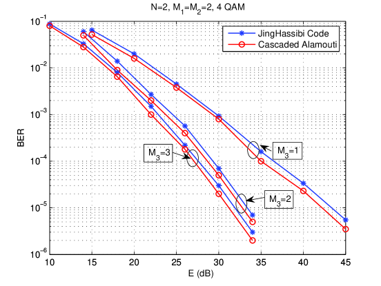
Figure 3: BER comparison of Cascaded Alamouti code with JingHassibi code for $N=2$-hop network

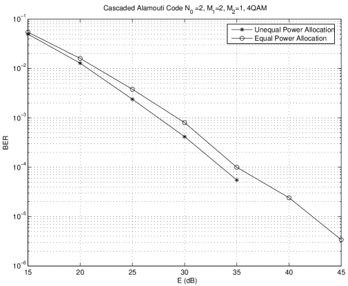
Figure 4: Performance of cascaded Alamouti with varying power allocation

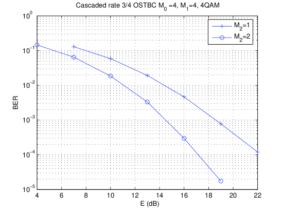
Figure 5: Cascaded rate 3/4 4 antenna OSTBC for $M_{0}=M_{1}=4$

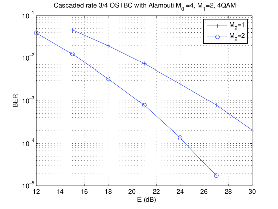
Figure 6: Cascaded rate 3/4 4 antenna OSTBC with Alamouti Code for $M_{0}=M_{1}=4$

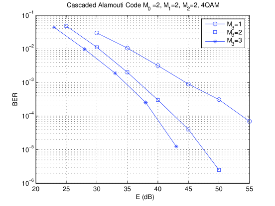
Figure 7: Cascaded Alamouti Code for $N=3$-hop network

VIII Conclusion

In this paper we designed DSTBC’s for multi-hop wireless network and analyzed their diversity gain. We assumed that receive CSI is known at each relay and the destination. We proposed an AF strategy called COSTBC to design DSTBC using OSTBC to communicate between adjacent relay stages when CSI is available at each relay. We showed that the COSTBCs achieve the maximum diversity gain in a multi-hop wireless network. We also showed that COSTBCs are single symbol decodable similar to OSTBC and thus incur minimum decoding complexity. We then gave an explicit construction of COSTBCs for various numbers of source, destination, and relay antennas that were shown to achieve maximum diversity gain with minimal encoding complexity. The only restriction that COSTBCs impose is that the source and all the relay stages have to use an OSTBC. It is well known that high rate OSTBC do not exist, therefore the COSTBCs have rate limitations. For future work it will be interesting to see whether the OSTBC requirement can be relaxed without sacrificing the maximum diversity gain and minimum decoding complexity of the COSTBCs.

Appendix A Single Symbol Decodable Property Of Cascaded Alamouti Code

In this section of the Appendix we show that COSTBCs (cascaded Alamouti code, Example 1) have the single symbol decodable property for a $N$-hop network when $M_{0}=\ldots=M_{N-1}=2$. We first establish this for $N=2$ and then generalize it to arbitrary $N$ using mathematical induction.

To construct COSTBC for $N=2,M_{0}=M_{1}=2$, let ${\mathbf{S}}_{0}$ be the Alamouti code which is given by:

$$\left[\begin{array}[]{cc}s_{1}&s_{2}\\ -s_{2}^{*}&s_{1}^{*}\end{array}\right]$$

where $s_{1}$ and $s_{2}$ are constituent symbols. Then the $2\times 1$ received signal at each relay is

$$\left[\begin{array}[]{c}r_{m}^{1}\\ r_{m}^{2}\end{array}\right]=\sqrt{E_{0}}\left[\begin{array}[]{cc}s_{1}&s_{2}\\ -s_{2}^{*}&s_{1}^{*}\end{array}\right]\left[\begin{array}[]{c}h_{1m}\\ h_{2m}\end{array}\right]+\left[\begin{array}[]{c}n_{m}^{1}\\ n_{m}^{2}\end{array}\right]$$

for $m=1,2$. Transforming

$$\left[\begin{array}[]{c}r_{m}^{1}\\ -r_{m}^{2*}\end{array}\right]=\sqrt{E_{0}}\underbrace{\left[\begin{array}[]{cc}h_{1m}&h_{2m}\\ -h_{2m}^{*}&h_{1m}^{*}\end{array}\right]}_{\tilde{{\mathbf{H}}}_{m}}\left[\begin{array}[]{c}s_{1}\\ s_{2}\end{array}\right]+\left[\begin{array}[]{c}n_{m}^{1}\\ -n_{m}^{2*}\end{array}\right]$$

for $m=1,2$. Premultiplying by ${\tilde{{\mathbf{H}}}^{*}_{m}}$

$$\left[\begin{array}[]{c}\tilde{r}_{m}^{1}\\ \tilde{r}_{m}^{2*}\end{array}\right]=\sqrt{E_{0}}\underbrace{\left[\begin{array}[]{cc}|h_{1m}|^{2}+|h_{2m}|^{2}&0\\ 0&|h_{1m}|^{2}+|h_{2m}|^{2}\end{array}\right]}_{{\mathsf{H}}_{m}}\left[\begin{array}[]{c}s_{1}\\ s_{2}\end{array}\right]+\underbrace{\left[\begin{array}[]{c}n_{m}^{1}h_{1m}^{*}+n_{m}^{2*}h_{2m}\\ n_{m}^{1}h_{2m}^{*}-n_{m}^{2*}h_{1m}\end{array}\right]}_{\tilde{{\mathbf{n}}}_{m}}$$ (29)

for $m=1,2$. Now premultiplying by $\mathsf{H}_{m}^{-\frac{1}{2}}$

$$\left[\begin{array}[]{c}\hat{r}_{m}^{1}\\ \hat{r}_{m}^{2*}\end{array}\right] = \sqrt{E_{0}}\underbrace{\left[\begin{array}[]{cc}\sqrt{|h_{1m}|^{2}+|h_{2m}|^{2}}&0\\ 0&\sqrt{|h_{1m}|^{2}+|h_{2m}|^{2}}\end{array}\right]}_{{\hat{\mathbf{H}}}_{m}}\left[\begin{array}[]{c}s_{1}\\ s_{2}\end{array}\right]$$ (38)

$$+\underbrace{\frac{1}{\sqrt{|h_{1m}|^{2}+|h_{2m}|^{2}}}\left[\begin{array}[]{c}n_{m}^{1}h_{1m}^{*}+n_{m}^{2*}h_{2m}\\ n_{m}^{1}h_{2m}^{*}-n_{m}^{2*}h_{1m}\end{array}\right]}_{\hat{{\mathbf{n}}}_{m}}$$

for $m=1,2$. It is easy to check that the entries of vector ${\hat{\mathbf{n}}}_{m}$ are ${\cal CN}(0,1)$ distributed and uncorrelated with each other from which it follows that entries of vector ${\hat{\mathbf{n}}}_{m}$ are independent. Using

$${\mathbf{A}}_{1}=\left[\begin{array}[]{cc}1&0\\ 0&1\end{array}\right],{\mathbf{B}}_{1}={\bf 0}_{2},\ {\mathbf{A}}_{2}={\bf 0}_{2},\ {\mathbf{B}}_{2}=\left[\begin{array}[]{cc}0&-1\\ 1&0\end{array}\right]$$

the $2\times 1$ transmitted signal from relay $1$ and $2$ is given by

$${\mathbf{t}}_{1} = \theta_{1}\left[\begin{array}[]{c}\sqrt{|h_{11}|^{2}+|h_{21}|^{2}}s_{1}\\ \sqrt{|h_{11}|^{2}+|h_{21}|^{2}}s_{2}\end{array}\right]+\frac{\theta_{2}}{\sqrt{|h_{11}|^{2}+|h_{21}|^{2}}}\left[\begin{array}[]{c}n_{1}^{1}h_{11}^{*}+n_{1}^{2*}h_{21}\\ n_{1}^{1}h_{21}^{*}-n_{1}^{2*}h_{11}\end{array}\right]$$ (43)

$${\mathbf{t}}_{2} = \theta_{1}\left[\begin{array}[]{c}-\sqrt{|h_{12}|^{2}+|h_{22}|^{2}}s_{2}^{*}\\ \sqrt{|h_{12}|^{2}+|h_{22}|^{2}}s_{1}^{*}\end{array}\right]+\frac{\theta_{2}}{\sqrt{|h_{12}|^{2}+|h_{22}|^{2}}}\left[\begin{array}[]{c}-(n_{2}^{1}h_{22}^{*}-n_{2}^{2*}h_{12})^{*}\\ (n_{2}^{1}h_{12}^{*}+n_{2}^{2*}h_{22})^{*}\end{array}\right],$$ (48)

where $\theta_{1}$ and $\theta_{2}$ are the scaling factors so that the power transmitted by each relay is $E_{1}$, ${\mathbb{E}}{\mathbf{t}}_{m}^{*}{\mathbf{t}}_{m}=E_{1}M_{1},\ m=1,2$. Recall from the COSTBC construction that ${\mathbf{S}}_{1}:=[{\mathbf{A}}_{1}{\mathbf{s}}+{\mathbf{B}}_{1}{\mathbf{s}}^{{\dagger}}\ \ {\mathbf{A}}_{2}{\mathbf{s}}+{\mathbf{B}}_{2}{\mathbf{s}}^{{\dagger}}]$, where ${\mathbf{s}}=[s_{1},s_{2},\ldots,s_{L}]$ is the vector of the constituent symbols of ${\mathbf{S}}_{0}$. In this case ${\mathbf{s}}=[s_{1},s_{2}]$ and ${\mathbf{S}}_{1}$ is

$$\left[\begin{array}[]{cc}s_{1}&-s_{2}^{*}\\ s_{2}&s_{1}^{*}\end{array}\right]$$

which is the Alamouti code and hence an OSTBC as required.

The $2\times 1$ received signal at the $j^{th}$ receive antenna of the destination is given by

$$\left[\begin{array}[]{c}y_{j}^{1}\\ y_{j}^{2}\end{array}\right] = \theta_{1}\left[\begin{array}[]{c}g_{1j}\sqrt{|h_{11}|^{2}+|h_{21}|^{2}}s_{1}-g_{2j}\sqrt{|h_{12}|^{2}+|h_{22}|^{2}}s_{2}^{*}\\ g_{1j}\sqrt{|h_{11}|^{2}+|h_{21}|^{2}}s_{2}+g_{2j}\sqrt{|h_{12}|^{2}+|h_{22}|^{2}}s_{1}^{*}\end{array}\right]$$

$$+\theta_{2}\left[\begin{array}[]{c}\frac{g_{1j}(n_{1}^{1}h_{11}^{*}+n_{1}^{2*}h_{21})}{\sqrt{|h_{11}|^{2}+|h_{21}|^{2}}}-\frac{g_{2j}(n_{2}^{1}h_{22}^{*}-n_{2}^{2*}h_{12})^{*}}{\sqrt{|h_{12}|^{2}+|h_{22}|^{2}}}\\ \frac{g_{1j}(n_{1}^{1}h_{21}^{*}-n_{1}^{2*}h_{11})}{\sqrt{|h_{11}|^{2}+|h_{21}|^{2}}}+\frac{g_{2j}(n_{2}^{1}h_{12}^{*}+n_{2}^{2*}h_{22})^{*}}{\sqrt{|h_{12}|^{2}+|h_{22}|^{2}}}\end{array}\right]+\left[\begin{array}[]{c}z_{j}^{1}\\ z_{j}^{2}\end{array}\right]$$

for $j=1,2$. We denote $\eta_{1}=\frac{(n_{1}^{1}h_{11}^{*}+n_{1}^{2*}h_{21})}{\sqrt{|h_{11}|^{2}+|h_{21}|^{2}}}$, $\eta_{2}=\frac{(n_{1}^{1}h_{21}^{*}-n_{1}^{2*}h_{11})}{\sqrt{|h_{11}|^{2}+|h_{21}|^{2}}}$, $\eta_{3}=\frac{(n_{2}^{1}h_{22}^{*}-n_{2}^{2*}h_{12})}{\sqrt{|h_{12}|^{2}+|h_{22}|^{2}}}$ $\eta_{4}=\frac{(n_{2}^{1}h_{12}^{*}+n_{2}^{2*}h_{22})}{\sqrt{|h_{12}|^{2}+|h_{22}|^{2}}}$. Note that ${{\mathbb{E}}}\eta_{i}\eta_{j}^{*}=0,\ \forall i,\ j=1,2,3,4\ i\neq j$. Rewriting,

$$\left[\begin{array}[]{c}y_{j}^{1}\\ y_{j}^{2*}\end{array}\right] = \theta_{1}\underbrace{\left[\begin{array}[]{cc}g_{1j}\sqrt{|h_{11}|^{2}+|h_{21}|^{2}}&-g_{2j}\sqrt{|h_{12}|^{2}+|h_{22}|^{2}}\\ g_{2j}^{*}\sqrt{|h_{12}|^{2}+|h_{22}|^{2}}&g_{1j}^{*}\sqrt{|h_{11}|^{2}+|h_{21}|^{2}}\end{array}\right]}_{\Phi_{j}}\left[\begin{array}[]{c}s_{1}\\ s_{2}^{*}\end{array}\right]$$

$$+\theta_{2}\left[\begin{array}[]{c}g_{1j}\eta_{1}-g_{2j}\eta_{3}^{*}\\ (g_{1j}\eta_{2}+g_{2j}\eta_{4}^{*})^{*}\end{array}\right]+\left[\begin{array}[]{c}z_{j}^{1}\\ z_{j}^{2*}\end{array}\right]$$

Denoting ${\tilde{h}}_{1}=|h_{11}|^{2}+|h_{21}|^{2}$ and ${\tilde{h}}_{2}=|h_{12}|^{2}+|h_{22}|^{2}$, premultiplying by $\Phi_{j}^{*}$, it follows that

$$\Phi_{j}^{*}\left[\begin{array}[]{c}y_{j}^{1}\\ y_{j}^{2*}\end{array}\right] = \theta_{1}\left[\begin{array}[]{cc}(|g_{1j}|^{2}{\tilde{h}}_{1}+|g_{2j}|^{2}{\tilde{h}}_{2})s_{1}\\ (|g_{1j}|^{2}{\tilde{h}}_{1}+|g_{2j}|^{2}{\tilde{h}}_{2})s_{2}\end{array}\right]$$

$$+\theta_{2}\underbrace{\Phi_{j}^{*}\left[\begin{array}[]{c}g_{1j}\eta_{1}-g_{2j}\eta_{3}^{*}\\ (g_{1j}\eta_{2}+g_{2j}\eta_{4}^{*})^{*}\end{array}\right]+\Phi_{j}^{*}\left[\begin{array}[]{c}z_{j}^{1}\\ z_{j}^{2*}\end{array}\right]}_{{\mathbf{v}}_{j}}$$

Expanding ${\mathbf{v}}_{j}$, we have

$${\mathbf{v}}_{j}=\theta_{2}\left[\begin{array}[]{c}|g_{1j}|^{2}\sqrt{{\tilde{h}}_{1}}\eta_{1}-g_{1j}^{*}g_{2j}\sqrt{{\tilde{h}}_{1}}\eta_{3}^{*}+g_{1j}^{*}g_{2j}\sqrt{{\tilde{h}}_{2}}\eta_{2}^{*}+|g_{2j}|^{2}\sqrt{{\tilde{h}}_{2}}\eta_{4}\\ -g_{1j}g_{2j}^{*}\sqrt{{\tilde{h}}_{2}}\eta_{1}+|g_{2j}|^{2}\sqrt{{\tilde{h}}_{2}}\eta_{3}^{*}+|g_{1j}|^{2}\sqrt{{\tilde{h}}_{1}}\eta_{2}^{*}+g_{1j}g_{2j}^{*}\sqrt{{\tilde{h}}_{1}}\eta_{4}\end{array}\right]+\left[\begin{array}[]{c}g_{1j}^{*}\sqrt{{\tilde{h}}_{1}}z_{j}^{1}+g_{2j}^{*}\sqrt{{\tilde{h}}_{2}}z_{j}^{2*}\\ -g_{2j}^{*}\sqrt{{\tilde{h}}_{2}}z_{j}^{1}+g_{1j}^{*}\sqrt{{\tilde{h}}_{1}}z_{j}^{2*}\end{array}\right]$$

It is easy to check that ${{\mathbb{E}}}{\mathbf{v}}_{j1}{\mathbf{v}}_{j2}^{*}=0$, ${{\mathbb{E}}}\sum_{j=1}^{M_{2}}{\mathbf{v}}_{j1}\left(\sum_{j=1}^{M_{2}}{\mathbf{v}}_{j2}\right)^{*}=0$ and ${\mathbf{v}}_{ji},\ i=1,2$ is circularly symmetric complex Gaussian which implies that $\sum_{j=1}^{M_{2}}{\mathbf{v}}_{j1}$ and $\sum_{j=1}^{M_{2}}{\mathbf{v}}_{j2}$ are independent and thus both $s_{1}$ and $s_{2}$ can be decoded independently of each other without any loss in performance compared to joint decoding. Thus we conclude that cascaded Alamouti code has the single symbol decodable property for $N=2,M_{0}=M_{1}=2$.

To extend this result to the $N$-hop case we use mathematical induction where $M_{n}=2\ \forall n=0,1\ldots,N-1$. We have shown the result for $N=2$, thus we can start the induction. Let us assume that the result is true for $k$-hop network. From the induction hypothesis, the cascaded Alamouti code has the single symbol decodable property for $k$-hop network, which means that at the $j^{th}$ receive antenna $j=1,2$ of the destination of $k$-hop network, using CSI, the received signal ${\mathbf{y}}_{j}$ can be transformed into ${\hat{\mathbf{y}}}_{j}$, where

$${\hat{\mathbf{y}}}_{j}=\alpha\left[\begin{array}[]{c}c_{j}s_{1}\\ c_{j}s_{2}\end{array}\right]+\beta\left[\begin{array}[]{c}z_{j1}\\ z_{j2}\end{array}\right]$$

$c_{j}$ is the channel gain, $\alpha$ and $\beta$ are the scaling factors and $z_{j1},z_{j2}$ are noise terms which are complex Gaussian distributed with zero mean and $\sigma^{2}_{k}$ variance and are independent of each other. We extend the $k$-hop network to $k+1$ network by assuming that the actual destination is one more hop away and using the destination of the $k$-hop network as the $k^{th}$ relay stage with $2$ relays with a single antenna each. Then using

$${\mathbf{A}}_{1}=\left[\begin{array}[]{cc}1&0\\ 0&1\end{array}\right],{\mathbf{B}}_{1}={\bf 0}_{2},\ {\mathbf{A}}_{2}={\bf 0}_{2},\ {\mathbf{B}}_{2}=\left[\begin{array}[]{cc}0&-1\\ 1&0\end{array}\right]$$

at the two relays of the $k^{th}$ relay stage, the $2\times 1$ transmitted signals ${\mathbf{t}}_{1}$ and ${\mathbf{t}}_{2}$ from the relay $1$ and $2$ of the $k^{th}$ relay stage, respectively, are given by

$${\mathbf{t}}_{1}={\hat{\alpha}}\left[\begin{array}[]{c}c_{1}s_{1}\\ c_{1}s_{2}\end{array}\right]+{\hat{\beta}}\left[\begin{array}[]{c}z_{11}\\ z_{12}\end{array}\right]$$

$${\mathbf{t}}_{2}={\hat{\alpha}}\left[\begin{array}[]{c}-c_{2}s_{2}^{*}\\ c_{2}s_{1}^{*}\end{array}\right]+{\hat{\beta}}\left[\begin{array}[]{c}-z_{21}^{*}\\ z_{22}^{*}\end{array}\right]$$

where ${\hat{\alpha}}$ and ${\hat{\beta}}$ are such that ${\mathbb{E}}{\mathbf{t}}_{j}^{*}{\mathbf{t}}_{j}=E_{k}M_{k}$. Recall that these transmitted signals are similar to the transmitted signals by cascaded Alamouti code in the $N=2$ case (43) where $c_{1}=\sqrt{|h_{11}|^{2}+|h_{21}|^{2}}$, $c_{2}=\sqrt{|h_{12}|^{2}+|h_{22}|^{2}}$, $z_{11}=\frac{n_{1}^{1}h_{11}^{*}+n_{1}^{2*}h_{21}}{\sqrt{|h_{11}|^{2}+|h_{21}|^{2}}}$, $z_{12}=\frac{n_{1}^{1}h_{21}^{*}-n_{1}^{2*}h_{11}}{\sqrt{|h_{11}|^{2}+|h_{21}|^{2}}}$, $z_{21}=\frac{n_{2}^{1}h_{22}^{*}-n_{2}^{2*}h_{12}}{\sqrt{|h_{12}|^{2}+|h_{22}|^{2}}}$, $z_{22}=\frac{n_{2}^{1}h_{12}^{*}+n_{2}^{2*}h_{22}}{\sqrt{|h_{12}|^{2}+|h_{22}|^{2}}}$. Using similar arguments as in the $N=2$ case, it easily follows that cascaded Alamouti code has the single symbol decodable property for $k+1$-hop network from which we can conclude that cascaded Alamouti code has the single symbol decodable property for arbitrary $N$-hop networks with $M_{0}=\ldots=M_{N-1}=2$. In the next section we show that COSTBCs have the single symbol decodable property for an arbitrary $N$-hop network.

Appendix B Single Symbol Decodable Property Of COSTBC

In this section we show that COSTBCs have the single symbol decodable property. We first show this for $2$-hop networks and then generalize it to $N$-hop networks where $N$ is any arbitrary integer. Let ${\mathbf{S}}_{0}$ be the transmitted OSTBC from the source and ${\mathbf{s}}=[s_{1},\ldots,s_{L}]^{T}$ be the vector of the constituent symbols of ${\mathbf{S}}_{0}$. Then from (3), using CSI, the received signal ${\mathbf{r}}^{1}_{k}$ at the $k^{th}$ relay of relay stage $1$ can be transformed into ${\hat{\mathbf{r}}}^{1}_{k}$ where

$${\hat{\mathbf{r}}}_{k}^{1}=\sqrt{E_{0}}\underbrace{\left(\begin{array}[]{cccc}\sqrt{\sum_{m=1}^{M_{0}}|h_{mk}|^{2}}&0&0&0\\ 0&\sqrt{\sum_{m=1}^{M_{0}}|h_{mk}|^{2}}&0&0\\ 0&0&\ddots&0\\ 0&0&0&\sqrt{\sum_{m=1}^{M_{0}}|h_{mk}|^{2}}\\ \end{array}\right)}_{\mathsf{H}^{\frac{1}{2}}}{\mathbf{s}}+\hat{{\mathbf{n}}}_{k}$$

and the entries of ${\hat{\mathbf{n}}}_{k}$ are independent and ${\cal CN}(0,1)$ distributed. For $N=2$, from (III) the received signal at the $j^{th}$ antenna of the destination can be written as

$${\mathbf{y}}_{j}=[{\mathbf{t}}^{1}_{1}\ {\mathbf{t}}^{1}_{2}\ \ldots\ {\mathbf{t}}^{1}_{M_{1}}]{\mathbf{g}}_{j}+{\mathbf{z}}_{j}$$

for $j=1,2,\ldots M_{2}$, where ${\mathbf{t}}^{1}_{k}$ is the transmitted vector from relay $k$ (4) of relay stage $1$. The received signal ${\mathbf{y}}_{j}$ can also be written as

$${\mathbf{y}}_{j} = \sqrt{\frac{E_{0}E_{1}M}{L\gamma}}{\mathbf{S}}_{1}\left[\begin{array}[]{c}\sqrt{\sum_{m=1}^{M_{0}}|h_{m1}|^{2}}g_{1j}\\ \sqrt{\sum_{m=1}^{M_{0}}|h_{m2}|^{2}}g_{2j}\\ \vdots\\ \sqrt{\sum_{m=1}^{M_{0}}|h_{mM_{1}}|^{2}}g_{M_{1}j}\end{array}\right]$$

$$+\underbrace{\sqrt{\frac{E_{1}M_{1}}{L\gamma}}[{\mathbf{A}}_{1}\hat{n}_{1}+{\mathbf{B}}_{1}\hat{n}^{{\dagger}}_{1}\ {\mathbf{A}}_{2}\hat{n}_{2}+{\mathbf{B}}_{2}\hat{n}^{{\dagger}}_{2}\ \ldots\ {\mathbf{A}}_{M_{1}}\hat{n}_{M_{1}}+{\mathbf{B}}_{M_{1}}\hat{n}^{{\dagger}}_{M_{1}}]{\mathbf{g}}_{j}+{\mathbf{z}}_{j}}_{{\mathbf{w}}_{j}}$$

where ${\mathbf{S}}_{1}=[{\mathbf{A}}_{1}{\mathbf{s}}+{\mathbf{B}}_{1}{\mathbf{s}}^{{\dagger}}\ {\mathbf{A}}_{2}{\mathbf{s}}+{\mathbf{B}}_{2}{\mathbf{s}}^{{\dagger}}\ \ldots\ {\mathbf{A}}_{M_{1}}{\mathbf{s}}+{\mathbf{B}}_{M_{1}}{\mathbf{s}}^{{\dagger}}]$.

Since ${\mathbf{S}}_{1}$ is an OSTBC, invoking the single symbol decodable property of OSTBC (2) and using the fact that entries of ${\mathbf{w}}_{j}$ are independent, it follows that, using CSI, the received signal ${\mathbf{y}}_{j}$ can be transformed into ${\hat{\mathbf{y}}}_{j}$, where

$${\hat{\mathbf{y}}}_{j}=\sqrt{\frac{E_{0}E_{1}M_{1}}{L\gamma}}\left(\begin{array}[]{ccc}\sum_{k=1}^{M_{1}}|g_{kj}|^{2}\left(\sum_{m=1}^{M_{0}}|h_{mk}|^{2}\right)&0&0\\ 0&\ddots&0\\ 0&0&\sum_{k=1}^{M_{1}}|g_{kj}|^{2}\left(\sum_{m=1}^{M_{0}}|h_{mk}|\right)^{2}\\ \end{array}\right){\mathbf{s}}+\hat{{\mathbf{w}}}_{j}$$

and the entries of $\hat{{\mathbf{w}}}_{j}$ are independent. Thus, it is clear that all the constituent symbols $s_{1},\ldots,s_{L}$ can be separated with independent noise terms and we conclude that COSTBCs have the single symbol decodable property for a $2$-hop network. Using mathematical induction, similar to the Appendix A, it can be easily shown that COSTBCs also have the single symbol decodable property for arbitrary $N$-hop network and for brevity we omit it here.

References

[1]
S. Alamouti, “A simple transmit diversity technique for wireless
communications,” IEEE J. Sel. Areas Commun., vol. 16, no. 8, pp.
1451–1458, Oct. 1998.
[2]
V. Tarokh, H. Jafarkhani, and A. Calderbank, “Space-time block coding for
wireless communications: performance results,” IEEE J. Sel. Areas
Commun., vol. 17, no. 3, pp. 451–460, March 1999.
[3]
J. Laneman and G. Wornell, “Distributed space-time-coded protocols for
exploiting cooperative diversity in wireless networks,” IEEE Trans.
Inf. Theory, vol. 49, no. 10, pp. 2415–2425, Oct. 2003.
[4]
J. Laneman, D. Tse, and G. Wornell, “Cooperative diversity in wireless
networks: Efficient protocols and outage behavior,” IEEE Trans. Inf.
Theory, vol. 50, no. 12, pp. 3062–3080, Dec. 2004.
[5]
J. Yindi and B. Hassibi, “Distributed space-time coding in wireless relay
networks with multiple-antenna nodes, submitted,” IEEE Trans. Signal
Process., 2004.
[6]
R. Nabar, H. Bolcskei, and F. Kneubuhler, “Fading relay channels: performance
limits and space-time signal design,” IEEE J. Sel. Areas Commun.,
vol. 22, no. 6, pp. 1099–1109, Aug. 2004.
[7]
J. Yindi and B. Hassibi, “Distributed space-time coding in wireless relay
networks,” IEEE Trans. Wireless Commun., vol. 5, no. 12, pp.
3524–3536, Dec. 2006.
[8]
C. Yang and J.-C. Belfiore, “Optimal space time codes for the MIMO
amplify-and-forward cooperative channel,” IEEE Trans. Inf. Theory,
vol. 53, no. 2, pp. 647–663, Feb. 2007.
[9]
G. Susinder Rajan and B. Sundar Rajan, “A non-orthogonal distributed
space-time coded protocol, Part-I: Signal model and design criteria,” in
Proceedings of IEEE Information Theory Workshop, Oct. 22-26 2006, pp.
385–389.
[10]
——, “A non-orthogonal distributed space-time coded protocol, Part-II:
Code construction and DM-G tradeoff,” in Proceedings of IEEE
Information Theory Workshop, Oct. 22-26 2006, pp. 488–492.
[11]
M. Damen and R. Hammons, “Distributed space-time codes: relays delays and code
word overlays,” in ACM International Conference On Communications And
Mobile Computing 2007, Honolulu, Hawaii, USA, 12-16 Aug. 2007, pp. 354–357.
[12]
F. Oggier and B. Hassibi, “An algebraic family of distributed space-time codes
for wireless relay networks,” in IEEE International Symposium on
Information Theory, 2006, July 2006, pp. 538–541.
[13]
T. Kiran and B. Rajan, “Distributed space-time codes with reduced decoding
complexity,” in IEEE International Symposium on Information Theory,
2006, July 2006, pp. 542–546.
[14]
P. Elia and P. Vijay Kumar, “Approximately universal optimality over several
dynamic and non-dynamic cooperative diversity schemes for wireless
networks,” available at http://arxiv.org/pdf/cs.it/0512028, Dec 7,
2005.
[15]
J. Yindi and B. Hassibi, “Using orthogonal and quasi-orthogonal designs in
wireless relay networks,” IEEE Trans. Inf. Theory, vol. 53, no. 11,
pp. 4106–4118, Nov. 2007.
[16]
V. Tarokh, H. Jafarkhani, and A. Calderbank, “Space-time block codes from
orthogonal designs,” IEEE Trans. Inf. Theory, vol. 45, no. 5, pp.
1456–1467, July 1999.
[17]
F. Oggier and B. Hassibi, “Code design for multihop wireless relay networks,”
Oct. 2007, available on www.hindawi.com.
[18]
S. Yang and J. Belfiore, “Diversity of MIMO multihop relay channels,” Aug.
2007, available on http://arxiv.org/PScache/arxiv/pdf/0708/0708. 0386v1.pdf.
[19]
K. Sreeram, S. Birenjith, and P. Vijay Kumar, “Multi-hop cooperative wireless
networks: Diversity multiplexing tradeoff and optimal code design,” in
ITA Workshop, 27 Jan.-1 Feb. 2008. U.C. San Diego, 2008 available on
http://ita.ucsd.edu/workshop/08.
[20]
L. Zheng and D. Tse, “Diversity and multiplexing: A fundamental tradeoff in
multiple-antenna channels,” IEEE Trans. Inf. Theory, vol. 49,
no. 5, pp. 1073–1096, May 2003.
[21]
P. Elia, K. Kumar, S. Pawar, P. Kumar, and H.-F. Lu, “Explicit space-time
codes achieving the diversity-multiplexing gain tradeoff,” IEEE
Trans. Inf. Theory, vol. 52, no. 9, pp. 3869–3884, Sept. 2006.
[22]
B. Sethuraman, B. Rajan, and V. Shashidhar, “Full-diversity, high-rate
space-time block codes from division algebras,” IEEE Trans. Inf.
Theory, vol. 49, no. 10, pp. 2596–2616, Oct. 2003.
[23]
H. L. V. Trees, Detection, Estimation, and Modulation Theory - Part
I. New York: Wiley, 1968.
[24]
T. Cover and J. Thomas, Elements of Information Theory. John Wiley and Sons, 2004.
[25]
I. Gradshteyn and I. Ryzhik, Table of Integrals, Series, and
Products. Academic Press, 1994.