Transformation methods for evaluating approximations to the optimal exercise boundary for linear and nonlinear Black-Scholes equations

Abstract. The purpose of this survey chapter is to present a transformation technique that can be used in analysis and numerical computation of the early exercise boundary for an American style of vanilla options that can be modelled by class of generalized Black-Scholes equations. We analyze qualitatively and quantitatively the early exercise boundary for a linear as well as a class of nonlinear Black-Scholes equations with a volatility coefficient which can be a nonlinear function of the second derivative of the option price itself. A motivation for studying the nonlinear Black-Scholes equation with a nonlinear volatility arises from option pricing models taking into account e.g. nontrivial transaction costs, investor’s preferences, feedback and illiquid markets effects and risk from a volatile (unprotected) portfolio. We present a method how to transform the free boundary problem for the early exercise boundary position into a solution of a time depending nonlinear nonlocal parabolic equation defined on a fixed domain. We furthermore propose an iterative numerical scheme that can be used in order to find an approximation of the free boundary. In the case of a linear Black-Scholes equation we are able to derive a nonlinear integral equation for the position of the free boundary. We present results of numerical approximation of the early exercise boundary for various types of linear and nonlinear Black-Scholes equations and we discuss dependence of the free boundary on model parameters. Finally, we discuss an application of the transformation method for the pricing equation for American type of Asian options.

1 Introduction

According to the classical theory due to Black, Scholes and Merton the price of an option in an idealized financial market can be computed from a solution to the well-known Black–Scholes linear parabolic equation derived by Black and Scholes in [7], and, independently by Merton (see also Kwok [38], Dewynne et al. [16], Hull [30], Wilmott et al. [53]). Recall that a European call (put) option is the right but not obligation to purchase (sell) an underlying asset at the expiration price $E$ at the expiration time $T$. Assuming that the underlying asset $S$ follows a geometric Brownian motion

$$dS=(\varrho-q)Sdt+\sigma SdW,$$ (1)

where $\varrho$ is a drift, $q$ is the asset dividend yield rate, $\sigma$ is the volatility of the asset and $W$ is the standard Wiener process (cf. [38]), one can derive a governing partial differential equation for the price of an option. We remind ourselves that the equation for option’s price $V(S,t)$ is the following parabolic PDE:

$$\frac{\partial V}{\partial t}+(r-q)S\frac{\partial V}{\partial S}+\frac{\sigma^{2}}{2}S^{2}\frac{\partial^{2}V}{\partial S^{2}}-rV=0$$ (2)

where $\sigma$ is the volatility of the underlying asset price process, $r>0$ is the interest rate of a zero-coupon bond, $q\geq 0$ is the dividend yield rate. A solution $V=V(S,t)$ represents the price of an option if the price of an underlying asset is $S>0$ at time $t\in[0,T]$.

The case when the diffusion coefficient $\sigma>0$ in (2) is constant represents a classical Black–Scholes equation originally derived by Black and Scholes in [7]. On the other hand, if we assume the volatility coefficient $\sigma>0$ to be a function of the solution $V$ itself then (2) with such a diffusion coefficient represents a nonlinear generalization of the Black–Scholes equation. It is a purpose of this chapter to focus our attention to the case when the diffusion coefficient $\sigma^{2}$ may depend on the time $T-t$ to expiry, the asset price $S$ and the second derivative $\partial^{2}_{S}V$ of the option price (hereafter referred to as $\Gamma$), i.e.

$$\sigma=\sigma(S^{2}\partial^{2}_{S}V,S,T-t)\,.$$ (3)

A motivation for studying the nonlinear Black–Scholes equation (2) with a volatility $\sigma$ having a general form (3) arises from option pricing models taking into account nontrivial transaction costs, market feedbacks and/or risk from a volatile (unprotected) portfolio. Recall that the linear Black–Scholes equation with constant $\sigma$ has been derived under several restrictive assumptions like e.g. frictionless, liquid and complete markets, etc. We also recall that the linear Black–Scholes equation provides a perfectly replicated hedging portfolio. In the last decades some of these assumptions have been relaxed in order to model, for instance, the presence of transaction costs (see e.g. Leland [39], Hoggard et al. [29], Avellaneda and Paras [4]), feedback and illiquid market effects due to large traders choosing given stock-trading strategies (Frey and Patie [22], Frey and Stremme [23], During et al.[17], Schönbucher and Wilmott [49]), imperfect replication and investor’s preferences (Barles and Soner [8]), risk from unprotected portfolio (Kratka [37], Jandačka and Ševčovič [32] or [47]). One of the first nonlinear models is the so-called Leland model (cf. [39]) for pricing call and put options under the presence of transaction costs. It has been generalized for more complex option strategies by Hoggard, Whaley and Wilmott in [29]. In this model the volatility $\sigma$ is given by

$$\sigma^{2}(S^{2}\partial^{2}_{S}V,S,\tau)=\hat{\sigma}^{2}(1+\hbox{Le}\,\hbox{sgn}(\partial^{2}_{S}V))$$ (4)

where $\hat{\sigma}>0$ is a constant historical volatility of the underlying asset price process and $\hbox{Le}>0$ is the so-called Leland constant given by $\hbox{Le}=\sqrt{2/\pi}C/(\hat{\sigma}\sqrt{\Delta t})$ where $C>0$ is a constant round trip transaction cost per unit dollar of transaction in the assets market and $\Delta t>0$ is the time-lag between portfolio adjustments.

Notice that dependence of volatility adjustment on the second derivative of the price is quite natural. Indeed, in the idealized Black-Scholes theory, the optimal hedge is equal to $\pm\partial_{S}V$ and therefore one may expect more frequent transaction in regions with the high second derivative $\partial^{2}_{S}V$ (cf. [7]).

A popular nonlinear generalization of the Black–Scholes equation has been proposed by Avellaneda, Levy, and Paras [5] for description of incomplete markets and uncertain but bounded volatility. In their model we have

$$\sigma^{2}(S^{2}\partial^{2}_{S}V,S,\tau)=\left\{\begin{array}[]{cc}\hat{\sigma}^{2}_{1}&\quad\hbox{if}\ \partial^{2}_{S}V<0,\\ \hat{\sigma}^{2}_{2}&\quad\hbox{if}\ \partial^{2}_{S}V>0,\end{array}\right.$$ (5)

where $\sigma_{1}$ and $\sigma_{2}$ represent a lower and upper a-priori bound on the otherwise unspecified asset price volatility.

If transaction costs are taken into account perfect replication of the contingent claim is no longer possible and further restrictions are needed in the model. By assuming that investor’s preferences are characterized by an exponential utility function Barles and Soner (cf. [8]) derived a nonlinear Black–Scholes equation with the volatility $\sigma$ given by

$$\sigma^{2}(S^{2}\partial^{2}_{S}V,S,\tau)=\hat{\sigma}^{2}\left(1+\Psi(a^{2}e^{r\tau}S^{2}\partial^{2}_{S}V)\right)$$ (6)

where $\Psi$ is a solution to the ODE: $\Psi^{\prime}(x)=(\Psi(x)+1)/(2\sqrt{x\Psi(x)}-x),\Psi(0)=0,$ and $a>0$ is a given constant representing risk aversion. Notice that $\Psi(x)=O(x^{\frac{1}{3}})$ for $x\to 0$ and $\Psi(x)=O(x)$ for $x\to\infty$.

Another popular model has been derived for the case when the asset dynamics takes into account the presence of feedback and illiquid market effects. Frey and Stremme (cf. [23, 22]) introduced directly the asset price dynamics in the case when a large trader chooses a given stock-trading strategy (see also [49]). The diffusion coefficient $\sigma$ is again nonconstant and it can be expressed as:

$$\sigma^{2}(S^{2}\partial^{2}_{S}V,S,\tau)=\hat{\sigma}^{2}\left(1-\varrho\lambda(S)S\partial^{2}_{S}V\right)^{-2}$$ (7)

where $\hat{\sigma}^{2},\varrho>0$ are constants and $\lambda(S)$ is a strictly convex function, $\lambda(S)\geq 1$. Interestingly enough, explicit solutions to the Black–Scholes equation with varying volatility as in (7) have been derived by Bordag and Chankova[9] and Bordag and Frey [10].

The last example of the Black–Scholes equation with a nonlinearly depending volatility is the so-called Risk Adjusted Pricing Methodology model proposed by Kratka in [37] and revisited by Jandačka and Ševčovič in [32]. In order to maintain (imperfect) replication of a portfolio by the delta hedge one has to make frequent portfolio adjustments leading to a substantial increase in transaction costs. On the other hand, rare portfolio adjustments may lead to an increase of the risk arising from a volatile (unprotected) portfolio. In the RAPM model the aim is to optimize the time-lag $\Delta t$ between consecutive portfolio adjustments. By choosing $\Delta t>0$ in such way that the sum of the rate of transaction costs and the rate of a risk from unprotected portfolio is minimal one can find the optimal time lag $\Delta t>0$. In the RAPM model, it turns out that the volatility is again nonconstant and it has the following form:

$$\sigma^{2}(S^{2}\partial^{2}_{S}V,S,\tau)=\hat{\sigma}^{2}\left(1+\mu(S\partial^{2}_{S}V)^{\frac{1}{3}}\right)\,.$$ (8)

Here $\hat{\sigma}^{2}>0$ is a constant historical volatility of the asset price returns and $\mu=3(C^{2}R/2\pi)^{\frac{1}{3}}$ where $C,R\geq 0$ are nonnegative constant representing the transaction cost measure and the risk premium measure, resp. (see [32] for details).

Notice that all the above mentioned nonlinear models are consistent with the original Black–Scholes equation in the case the additional model parameters (e.g. Le, $a$, $\varrho$, $\mu$) are vanishing. If plain call or put vanilla options are concerned then the function $V(S,t)$ is convex in $S$ variable and therefore each of the above mentioned models has a diffusion coefficient strictly larger than $\hat{\sigma}^{2}$ leading to a larger values of computed option prices. They can be therefore identified with higher Ask option prices, i.e. offers to sell an option. Furthermore, these models have been considered and analyzed mostly for European style of options, i.e. options that can be exercised only at the maturity $t=T$. On the other hand, American options are much more common in financial markets as they allow for exercising of an option anytime before the expiry $T$. In the case of an American call option a solution to equation (2) is defined on a time dependent domain $0<S<S_{f}(t),\ 0<t<T$. It is subject to the boundary conditions

$$V(0,t)=0\,,\ \ V(S_{f}(t),t)=S_{f}(t)-E\,,\ \ \partial_{S}V(S_{f}(t),t)=1\,,$$ (9)

and terminal pay-off condition at expiry $t=T$

$$V(S,T)=\max(S-E,0)$$ (10)

where $E>0$ is a strike price (cf. [16, 38]). One of important problems in this field is the analysis of the early exercise boundary $S_{f}(t)$ and the optimal stopping time (an inverse function to $S_{f}(t)$) for American call (or put) options on stocks paying a continuous dividend yield with a rate $q>0$ (or $q\geq 0$). However, an exact analytical expression for the free boundary profile is not even known for the case when the volatility $\sigma$ is constant. Many authors have investigated various approximation models leading to approximate expressions for valuing American call and put options: analytic approximations (Barone–Adesi and Whaley [6], Kuske and Keller [36], Dewynne et al. [16], Geske et al. [24, 25], MacMillan [40], Mynemi [44]); methods of reduction to a nonlinear integral equation (Alobaidi [1], Kwok [38], Mallier et al. [41, 42], Ševčovič [46], Stamicar et al. [50]). In recent papers [55, 56], Zhu derived a closed form of the free boundary position in terms of on infinite series. We also refer to a recent survey paper by Chadam [12] focusing on free boundary problems in mathematical finance.

We remind ourselves that in the case of a constant volatility there are, in principle, two ways how to solve numerically the free boundary problem for the value of an American call resp. put option and the position of the early exercise boundary. The first class of algorithms is based on reformulation of the problem in terms of a variational inequality (see Kwok [38] and references therein). The variational inequality can be then solved numerically by the so-called Projected Super Over Relaxation method (PSOR for short). An advantage of this method is that it gives us immediately the value of a solution. A disadvantage is that one has to solve large systems of linear equations iteratively taking into account the obstacle for a solution, and, secondly, the free boundary position should be deduced from the solution a posteriori. Moreover, the PSOR method is not directly applicable for solving the problem (2)-(9) when the diffusion coefficient $\sigma$ may depend on the second derivative of a solution itself. The second class of methods is based on derivation of a nonlinear integral equation for the position of the free boundary without the need of knowing the option price itself (see e.g. Evans, Kuske-Keller [21, 36], Mallier and Alobaidi [1, 41, 42], Ševčovič et al. [46, 50], Chadam et al. [12, 13]. In this approach an advantage is that only a single equation for the free boundary has to be solved provided that $\sigma$ is constant; a disadvantage is that the method is based on integral transformation techniques and therefore the assumption $\sigma$ is constant is crucial.

Higher order finite difference approximations of the free boundary problems for call or put options are discussed in recent papers by Ankudinova and Ehrhardt [2, 3], Ehrhardt and Mickens [18] and Zhao et al. [54]. Other interesting analytical and numerical methods for evaluating the early exercise boundary have been recently studied by e.g. Milstein et al. [43] (Monte–Carlo methods), Widdicks et al. [52] (singular pertubation techniques and asymptotic expansions), Cho et al. [14] (parameter estimation methods), Grandits and Schachinger et al. [26] (tracking of a discontinuity method), Imai et al. [31] (numerical method for generalized Lelend model).

In this survey we recall an iterative numerical algorithm for solving the free boundary problem for an American type of options in the case the volatility $\sigma$ may depend on the option and asset values as well as on the time $T-t$ to expiry as well as for American type of Asian options. A key idea of this method consists in transformation of the free boundary problem into a semilinear parabolic equation defined on a fixed spatial domain coupled with a nonlocal algebraic constraint equation for the free boundary position. It has been proposed and analyzes by the author in a series of papers [50, 46, 47, 48]. Since the resulting parabolic equation contains a strong convective term we make use of the operator splitting method in order to overcome numerical difficulties. A full space-time discretization of the problem leads to a system of semi-linear algebraic equations that can be solved by an iterative procedure at each time level.

The rest of the chapter has the following organization: in the next section we recall the well known nonlinear generalization of Black–Scholes equations due to Frey and Stremme, Barles and Soner and Kratka, Jandačka and Ševčovič, resp. We also present qualitative and quantitative properties of the nonlinear models for pricing European style of options with special focus on the Risk adjusted pricing methodology (RAPM) due to Kratka [37], Jandačka and Ševčovič [32]. Section 3 is devoted to the free boundary problem for pricing American options by means of a linear Black–Scholes equation, i.e. $\sigma>0$ is constant. This is important in order to understand important steps of the fixed domain transformation method. A resulting system of transformed equations consists of a nonlocal parabolic equation defined on a fixed domain with time depending coefficients and an algebraic constraint equation for the free boundary position. Since the volatility $\sigma$ is constant in this case, by using Sine and Cosine Fourier transformations the system of transformed equations can be further simplified and reduced to a single nonlinear integral equation for the free boundary position. We show how this integral equation can be utilized in order to obtain qualitative properties of the free boundary position (early exercise behavior, long time behavior) as well as quantitative properties (a fast and stable numerical scheme for computing the free boundary function). In Section 4 we discuss a transformation method applied to a class of nonlinear Black–Scholes equations. We are able to derive a similar system of transformed parabolic–algebraic equation to the one from Section 3. However, as the volatility is no longer a constant and it may depend on the solution itself the resulting system of equations can not be reduced to a single integral equation for the free boundary and it has to be solved numerically. We propose a numerical method based on the finite difference approximation combined with an operator splitting technique for numerical approximation of the solution and computation of the free boundary position. Several numerical results for nonlinear Black–Scholes equations with volatility functions $\sigma$ defined as in (6) and (8) are presented. We also compare our methodology with well-known methods for evaluation of approximation to the free boundary position in the case the volatility $\sigma$ is constant. We analyze dependence of the free boundary position with respect to various parameters entering expressions (6) and (8). Finally, Section 5 is devoted to a recent application of the transformation method in the case of American style of Asian options in which the strike price is an arithmetical average of underlying asset prices. Although the volatility $\sigma$ is assumed to be constant, due to a specific character of the Black–Scholes equation for pricing Asian option the resulting transformed system of equation cannot be further reduced and has to be solved numerically by a slight modification of the numerical method discussed in Section 4. We finish the last section by presentation of several illustrative examples describing the early exercise boundary for American style of Asian call options with floating strike.

2 Risk adjusted methodology model

The aim of this section is to present one of nonlinear generalizations of the classical Black–Scholes equation with a volatility $\sigma$ of the form (3) in a more detail. We focus on the so-called Risk adjusted pricing methodology model due to Kratka [37] and straightforward generalization by Jandačka and Ševčovič [32] (see also [47]). In this model both the risk arising from nontrivial transaction costs as well as the risk from unprotected volatile portfolio are taken into account. Their sum representing the total risk is subject of minimization. The original model was proposed by [37]. In [32] we modified Kratka’s approach by considering a different measure for risk arising from unprotected portfolio in order to construct a model which is scale invariant and mathematically well posed. These two important features were missing in the original model of Kratka. The model is based on the Black–Scholes parabolic PDE in which transaction costs are described by the Hoggard, Whalley and Wilmott extension of the Leland model (cf. [29, 38, 30]) whereas the risk from a volatile portfolio is described by the average value of the variance of the synthesized portfolio. Transaction costs as well as the volatile portfolio risk depend on the time-lag between two consecutive transactions. We define the total risk premium as a sum of transaction costs and the risk cost from the unprotected volatile portfolio. By minimizing the total risk premium functional we obtain the optimal length of the hedge interval.

Concerning the dynamics of an underlying asset we will assume that the asset price $S=S(t),t\geq 0,$ follows a geometric Brownian motion (1) with a drift $\rho$, standard deviation $\hat{\sigma}>0$ and it may pay continuous dividends, i.e. $dS=(\rho-q)Sdt+\hat{\sigma}SdW$ where $dW$ denotes the differential of the standard Wiener process and $q\geq 0$ is a continuous dividend yield rate. This assumption is usually made when deriving the classical Black–Scholes equation (see e.g. [30, 38]). Similarly as in the derivation of the classical Black–Scholes equation we construct a synthesized portfolio $\Pi$ consisting of a one option with a price $V$ and $\delta$ assets with a price $S$ per one asset:

$$\Pi=V+\delta S\,.$$ (11)

We recall that the key idea in the Black–Scholes theory is to examine the differential $\Delta\Pi$ of equation (11). The right-hand side of (11) can be differentiated by using Itô’s formula whereas portfolio’s increment $\Delta\Pi(t)=\Pi(t+\Delta t)-\Pi(t)$ of the left-hand side can be expressed as follows:

$$\Delta\Pi=r\Pi\Delta t+\delta qS\Delta t$$ (12)

where $r>0$ is a risk-free interest rate of a zero-coupon bond. In the real world, such a simplified assumption is not satisfied and a new term measuring the total risk should be added to (12). More precisely, the change of the portfolio $\Pi$ is composed of two parts: the risk-free interest rate part $r\Pi\Delta t$ and the total risk premium: $r_{R}S\Delta t$ where $r_{R}$ is a risk premium per unit asset price. We consider a short positioned call option. Therefore the writer of an option is exposed to this total risk. Hence we are going to price the higher Ask option price – an offer to sell an option. It means that $\Delta\Pi=r\Pi\Delta t-r_{R}S\Delta t$. The total risk premium $r_{R}$ consists of the transaction risk premium $r_{TC}$ and the portfolio volatility risk premium $r_{VP}$, i.e. $r_{R}=r_{TC}+r_{VP}$. Hence

$$\Delta\Pi=r\Pi\Delta t+\delta qS\Delta t-(r_{TC}+r_{VP})S\Delta t\,.$$ (13)

Our next goal is to show how these risk premium measures $r_{TC},$ $r_{VP}$ depend on the time lag and other quantities, like e.g. $\hat{\sigma},S,V,$ and derivatives of $V.$ The problem can be decomposed in two parts: modeling the transaction costs measure $r_{TC}$ and volatile portfolio risk measure $r_{VP}$.

We begin with modeling transaction costs. In practice, we have to adjust our portfolio by frequent buying and selling of assets. In the presence of nontrivial transaction costs, continuous portfolio adjustments may lead to infinite total transaction costs. A natural way how to consider transaction costs within the frame of the Black–Scholes theory is to follow the well known Leland approach extended by Hoggard, Whalley and Wilmott (cf. [29, 38]). We will recall an idea how to incorporate the effect of transaction costs into the governing equation. More precisely, we will derive the coefficient of transaction costs $r_{TC}$ occurring in (13). Let us denote by $C$ the round trip transaction cost per unit dollar of transaction. Then

$$C=(S_{ask}-S_{bid})/S$$ (14)

where $S_{ask}$ and $S_{bid}$ are the so-called Ask and Bid prices of the asset, i.e. the market price offers for selling and buying assets, resp. Here $S=(S_{ask}+S_{bid})/2$ denotes the mid value of the underlying asset price.

In order to derive the term $r_{TC}$ in (13) measuring transaction costs we will assume, for a moment, that there is no risk from volatile portfolio, i.e. $r_{VP}=0$. Then $\Delta V+\delta\Delta S=\Delta\Pi=r\Pi\Delta t+\delta qS\Delta t+r_{TC}S\Delta t$. Following Leland’s approach (cf. [29]), using Itô’s formula and assuming $\delta$-hedging of a synthetised portfolio $\Pi$ one can derive that the coefficient $r_{TC}$ of transaction costs is given by the formula:

$$r_{TC}=\frac{C\hat{\sigma}S}{\sqrt{2\pi}}\left|\partial^{2}_{S}V\right|\frac{1}{\sqrt{\Delta t}}$$ (15)

(see [29, Eq. (3)]). It leads to the well known Leland generalization of the Black–Scholes equation (2) in which the diffusion coefficient is given by (4) (see [39, 29] for details).

Next we focus our attention to the problem how to incorporate a risk from a volatile portfolio into the model. In the case when a portfolio consisting of options and assets is highly volatile, an investor usually asks for a price compensation. Notice that exposure to risk is higher when the time-lag between portfolio adjustments is higher. We shall propose a measure of such a risk based on the volatility of a fluctuating portfolio. It can be measured by the variance of relative increments of the replicating portfolio $\Pi=V+\delta S$, i.e. by the term $var((\Delta\Pi)/S)$. Hence it is reasonable to define the measure $r_{VP}$ of the portfolio volatility risk as follows:

$$r_{VP}=R\,\frac{var\left(\frac{\Delta\Pi}{S}\right)}{\Delta t}\,.$$ (16)

In other words, $r_{VP}$ is proportional to the variance of a relative change of a portfolio per time interval $\Delta t$. A constant $R$ represents the so-called risk premium coefficient. It can be interpreted as the marginal value of investor’s exposure to a risk. If we apply Itô’s formula to the differential $\Delta\Pi=\Delta V+\delta\Delta S$ we obtain $\Delta\Pi=\left(\partial_{S}V+\delta\right)\hat{\sigma}S\Delta W+{\scriptstyle\frac{1}{2}}\hat{\sigma}^{2}S^{2}\Gamma(\Delta W)^{2}+{\mathcal{G}}$ where $\Gamma=\partial_{S}^{2}V$ and ${\mathcal{G}}=(\partial_{S}V+\delta)\rho S\Delta t+\partial_{t}V\Delta t$ is a deterministic term, i.e $E({\mathcal{G}})={\mathcal{G}}$ in the lowest order $\Delta t$ - term approximation. Thus

$$\Delta\Pi-E(\Delta\Pi)=\left(\partial_{S}V+\delta\right)\hat{\sigma}S\phi\sqrt{\Delta t}+\frac{1}{2}\hat{\sigma}^{2}S^{2}(\phi^{2}-1)\Gamma\Delta t$$

where $\phi$ is a random variable with the standard normal distribution such that $\Delta W=\phi\sqrt{\Delta t}$. Hence the variance of $\Delta\Pi$ can be computed as follows:

$$var(\Delta\Pi)=E\left([\Delta\Pi-E(\Delta\Pi)]^{2}\right)=E\left([(\partial_{S}V+\delta)\hat{\sigma}S\phi\sqrt{\Delta t}+{\scriptstyle\frac{1}{2}}\hat{\sigma}^{2}S^{2}\Gamma\left(\phi^{2}-1\right)\Delta t]^{2}\right)\,.$$

Similarly, as in the derivation of the transaction costs measure $r_{TC}$ we assume the $\delta$-hedging of portfolio adjustments, i.e. we choose $\delta=-\partial_{S}V$. Since $E((\phi^{2}-1)^{2})=2$ we obtain an expression for the risk premium $r_{VP}$ in the form:

$$r_{VP}=\frac{1}{2}R\hat{\sigma}^{4}S^{2}\Gamma^{2}\Delta t\,.$$ (17)

Notice that in our approach the increase in the time-lag $\Delta t$ between consecutive transactions leads to a linear increase of the risk from a volatile portfolio where the coefficient of proportionality depends the asset price $S$, option’s Gamma, $\Gamma=\partial^{2}_{S}V$, as well as the constant historical volatility $\hat{\sigma}$ and the risk premium coefficient $R$.

2.1 Risk adjusted Black–Scholes equation

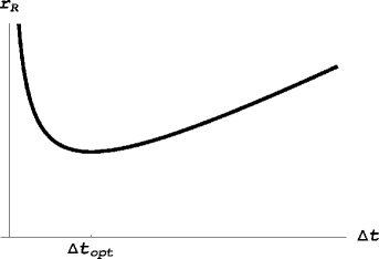
Figure 1: The total risk premium $r_{R}=r_{TC}+r_{VP}$ as a function of the time-lag $\Delta t$ between two consecutive portfolio adjustments.

The total risk premium $r_{R}=r_{TC}+r_{VP}$ consists of two parts: transaction costs premium $r_{TC}$ and the risk from a volatile portfolio $r_{VP}$ premium defined as in (15) and (17), resp. We assume that an investor is risk aversive and he/she wants to minimize the value of the total risk premium $r_{R}$. For this purpose one has to choose the optimal time-lag $\Delta t$ between two consecutive portfolio adjustments. As both $r_{TC}$ as well as $r_{VP}$ depend on the time-lag $\Delta t$ so does the total risk premium $r_{R}$. In order to find the optimal value of $\Delta t$ we have to minimize the following function:

$$\Delta t\mapsto r_{R}=r_{TC}+r_{VP}=\frac{C|\Gamma|\hat{\sigma}S}{\sqrt{2\pi}}\frac{1}{\sqrt{\Delta t}}+\frac{1}{2}R\hat{\sigma}^{4}S^{2}\Gamma^{2}\Delta t\,.$$

The unique minimum of the function $\Delta t\mapsto r_{R}(\Delta t)$ is attained at the time-lag $\Delta t_{opt}=K^{2}/(\hat{\sigma}^{2}|S\Gamma|^{\frac{2}{3}})$ where $K=(C/(R\sqrt{2\pi})^{\frac{1}{3}}$. For the minimal value of the function $\Delta t\mapsto r_{R}(\Delta t)$ we have

$$r_{R}(\Delta t_{opt})=\frac{3}{2}\left(\frac{C^{2}R}{2\pi}\right)^{\frac{1}{3}}\hat{\sigma}^{2}|S\Gamma|^{\frac{4}{3}}\,.$$ (18)

Taking into account both transaction costs as well as risk from a volatile portfolio effects we have shown that the equation for the change $\Delta\Pi$ of a portfolio $\Pi$ read as:

$$\Delta V+\delta\Delta S=\Delta\Pi\Delta t=r\Pi\Delta t+\delta qS\Delta t-r_{R}S\Delta t$$

where $r_{R}$ represents the total risk premium, $r_{R}=r_{TC}+r_{VP}$. Applying Itô’s lemma to a smooth function $V=V(S,t)$ and assuming the $\delta$-hedging strategy for the portfolio adjustments we finally obtain the following generalization of the Black–Scholes equation for valuing options:

$$\frac{\partial V}{\partial t}+\frac{\hat{\sigma}^{2}}{2}S^{2}\frac{\partial^{2}V}{\partial S^{2}}+(r-q)S\frac{\partial V}{\partial S}-rV-r_{R}S=0\,.$$

By taking the optimal value of the total risk coefficient $r_{R}$ derived as in (18) the option price $V$ is a solution to the following nonlinear parabolic equation:

(Risk adjusted Black–Scholes equation)

$$\frac{\partial V}{\partial t}+\frac{\hat{\sigma}^{2}}{2}S^{2}\left(1+\mu(S\partial^{2}_{S}V)^{\frac{1}{3}}\right)\frac{\partial^{2}V}{\partial S^{2}}+(r-q)S\frac{\partial V}{\partial S}-rV=0\,,$$ (19)

where $\mu=3\left(\frac{C^{2}R}{2\pi}\right)^{\frac{1}{3}}$ and $u^{p}$ with $u=S\partial^{2}_{S}V$ and $p=1/3$ stands for the signed power function, i.e. $u^{p}=|u|^{p-1}u$. In the case there are neither transaction costs ($C=0$) nor the risk from a volatile portfolio ($R=0$) we have $\mu=0$. Then equation (19) reduces to the original Black–Scholes linear parabolic equation (2). We note that equation (19) is a backward parabolic PDE if and only if the function $\beta(H)=\frac{\hat{\sigma}^{2}}{2}(1+\mu H^{\frac{1}{3}})H$ is an increasing function in the variable $H:=S\Gamma=S\partial^{2}_{S}V$. It is clearly satisfied if $\mu\geq 0$ and $H\geq 0$.

As it is usual in the classical Black-Scholes theory for European style of options (cf. [30, 38]) we consider the change of independent variables: $x:=\ln\left(\frac{S}{E}\right)\,,\ \ x\in\mathbb{R}\,,\qquad\tau:=T-t\,,\ \ \tau\in(0,T)\,.$ As equation (19) contains the term $S\Gamma=S\partial^{2}_{S}V$ it is convenient to introduce the following transformation: $H(x,\tau):=S\Gamma=S\partial^{2}_{S}V(S,t)$. Now we are in position to derive an equation for the function $H$. It turns out that the function $H(x,\tau)$ is a solution to a nonlinear parabolic equation subject to the initial and boundary conditions. More precisely, by taking the second derivative of equation (19) with respect to $x$ we obtain, after some calculations, that $H=H(x,\tau)$ is a solution to the quasilinear parabolic equation

$$\frac{\partial H}{\partial\tau}=\frac{\partial^{2}}{\partial x^{2}}\beta(H)+\frac{\partial}{\partial x}\beta(H)+r\frac{\partial H}{\partial x}\,,$$ (20)

$\tau\in(0,T),x\in\mathbb{R}$ (see [32]). Henceforth, we will refer to (20) as a $\Gamma$ equation. A solution $H$ to (20) is subjected to the initial condition at $\tau=0$:

$$H(x,0)=\bar{H}(x)\,,\quad x\in\mathbb{R}\,,$$ (21)

where $\bar{H}(x)$ is the Dirac $\delta$ function $\bar{H}(x)=\delta(x)$. For the purpose of numerical approximation we approximate the initial Dirac delta function by $\bar{H}(x)=N^{\prime}(d)/(\sigma\sqrt{\tau^{*}})$ where $\tau^{*}>0$ is sufficiently small, $N(d)$ is the cumulative distribution function of the normal distribution, and $d=\left(x+(r-q-\sigma^{2}/2)\tau^{*}\right/\sigma\sqrt{\tau^{*}})$. It corresponds to the value $H=S\partial^{2}_{S}V$ of a call (put) option valued by a linear Black–Scholes equation with a constant volatility $\sigma>0$ at the time $T-\tau^{*}$ close to expiry $T$ when the time parameter $0<\tau^{*}\ll 1$ is sufficiently small. In the case of call or put options the function $H$ is subjected to boundary conditions at $x=\pm\infty$,

$$H(-\infty,\tau)=H(\infty,\tau)=0\,,\quad\tau\in(0,T)\,.$$ (22)

A numerical discretization scheme of the $\Gamma$ equation (20) based on finite volume approximation has been discussed in [32] in more details.

2.2 Pricing of European style of options by the RAPM model

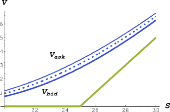
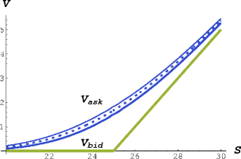
Figure 2: A comparison of Bid and Ask option prices computed by means of the RAPM model. The middle dotted line is the option price computed from the Black-Scholes equation. We chose $\sigma=0.3,\mu=0.2,r=0.011,E=25$ and $T=1$ (left) and $T=0.3$ (right).

Let us denote $V(S,t;C,\hat{\sigma},R)$ the value of a solution to (19) with parameters $C,\hat{\sigma},R$. Suppose that the coefficient of transaction costs $C$ is known from and is given by (14). In real option market data we can observe different Bid and Ask prices for an option, $V_{bid}<V_{ask}$, resp. Let us denote by $V_{mid}$ the mid value, i.e. $V_{mid}={\scriptstyle\frac{1}{2}}(V_{bid}+V_{ask})$. By the RAPM model we are able to explain such a Bid-Ask spread in option prices. The higher Ask price corresponds to a solution to the RAPM model with some nontrivial risk premium $R>0$ and $C>0$ whereas the mid value $V_{mid}$ corresponds to a solution $V(S,t)$ for vanishing risk premium $R=0$, i.e. to a solution of the linear Black-Scholes equation (2). An illustrative example of Bid-Ask spreads captured by the RAPM model is shown in Fig. 2.

To calibrate the RAPM model we seek for a couple $(\hat{\sigma}_{RAPM},R)$ of implied RAPM volatility $\sigma_{RAPM}$ and risk premium $R$ such that $V_{ask}=V(S,t;C,\hat{\sigma}_{RAPM},R)$ and $V_{mid}=V(S,t;C,\hat{\sigma}_{RAPM},0)$. Such a system of nonlinear equation for $\sigma_{RAPM}$ and $R$ can be solved by by means of the Newton-Kantorovich iterative method (cf. [32]).

As an example we considered sample data sets for call options on Microsoft stocks. We considered a flat interest rate $r=0.02$, a constant transaction cost coefficient $C=0.01$ estimated from (14), and we assumed that the underlying asset pays no dividends, i.e. $q=0$. In Fig. 3 we present results of calibration of implied couple $(\hat{\sigma}_{RAPM},R)$. Interestingly enough, two call options with higher strike prices $E=25,30$ had almost constant implied risk premium $R$. On the other the risk premium of an option with lowest $E=23$ was fluctuating and it had highest average of $R$.

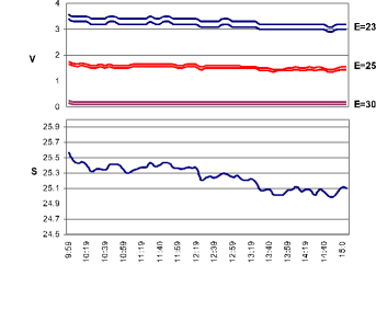
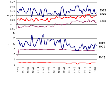
Figure 3: Intra-day behavior of Microsoft stocks (April 4, 2003) and shortly expiring call options with expiry date April 19, 2003. Computed implied volatilities $\hat{\sigma}_{RAPM}$ and risk premium coefficients $R$.

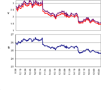
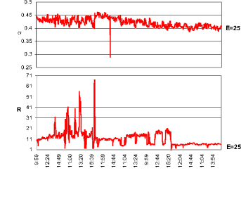
Figure 4: One week behavior of Microsoft stocks (March 20 - 27, 2003) and call options with expiration date April 19, 2003. Computed implied volatilities $\hat{\sigma}_{RAPM}$ and risk premiums $R$.

Finally, in Fig. 4 we present one week behavior of implied volatilities and risk premium coefficients for the Microsoft call option on $E=25$ expiring at $T=$ April 19, 2003. In the beginning of the investigated period the risk premium coefficient $R$ was rather high and fluctuating. On the other hand, it tends to a flat value of $R\approx 5$ at the end of the week. Interesting feature can be observed at the end of the second day when both stock and option prices went suddenly down. The time series analysis of the implied volatility $\hat{\sigma}_{RAPM}$ from first two days was unable to predict such a behavior. On the other, high fluctuation in the implied risk premium $R$ during first two days can send a signal to an investor that sudden changes can be expected in the near future.

3 Transformation method for a linear Black–Scholes equation

One of the interesting problems in this field is the analysis of the early exercise boundary and the optimal stopping time for American options on stocks paying a continuous dividend. It can be easily reduced to a problem of solving a certain free boundary problem for the Black–Scholes equation (cf. Black & Scholes [7]). However, the exact analytical expression for the free boundary profile is not known yet. Many authors have investigated various approximate models leading to approximate expressions for valuing American call and put options (see e.g. [24, 25, 33, 35, 36, 44, 45] and recent papers by Zhu [55, 56], Alobaidi et al.[1, 41, 42], Stamicar et al. [50] and the survey paper by Chadam [12] and other references therein). For the purpose of studying the free boundary profile near expiry, many different integral equations have been derived [6, 11, 30, 40].

Let us recall that the equation governing the time evolution of the price $V(S,t)$ of the American call option is the following parabolic PDE:

$${\partial V\over\partial t}+(r-q)S{\partial V\over\partial S}+{\sigma^{2}\over 2}S^{2}{\partial^{2}V\over\partial S^{2}}-rV=0\,,\qquad 0<S<S_{f}(t),\ 0<t<T\,,$$

$$V(0,t)=0,\ V(S_{f}(t),t)=S_{f}(t)-E\,,\ {\partial V\over\partial S}(S_{f}(t),t)=1\,,$$ (23)

$$V(S,T)=\max(S-E,0)\,,$$

defined on a time-dependent domain $S\in(0,S_{f}(t))$, where $t\in(0,T)$. As usual $S>0$ is the stock price, $E>0$ is the exercise price, $r>0$ is the risk-free rate, $q>0$ is the continuous stock dividend rate and

$$\sigma\equiv const>0$$

is a constant volatility of the underlying stock process.

The main purpose of this section is to present an alternative integral equation which will provide an accurate numerical method for calculating the early exercise boundary near expiry. The derivation of the nonlinear integral equation is based on the Fourier transform. A solution to this integral equation is the free boundary profile. The novelty of this approach consists in three steps:

1. The fixed domain transformation.

2. Derivation of a parabolic PDE for the so-called synthetic portfolio with a nonlinear nonlocal constraint between the free boundary position and the solution of this parabolic equation itself.

3. Construction of a solution by means of Fourier sine and cosine integral transforms.

Throughout this section we restrict our attention to the case when $r>q>0$. It is well known that, for $r>q>0$, the free boundary $\varrho(\tau)=S_{f}(T-\tau)$ starts at $\varrho(0)=rE/q$, whereas $\varrho(0)=E$ for the case $r\leq q$ (cf. Dewynne et al. [16], Kwok [38]). Thus, the free boundary profile develops an initial jump in the case $r>q>0$. Notice that the case $0<r\leq q$ can be also treated by other methods based on integral equations. Kwok [38] derived another integral equation which covers both cases $0<r\leq q$, as well as $r>q>0$ (see equation (48) and Remark 3.2). However, in the latter case equation (48) becomes singular as $t\to T^{-}$, leading to numerical instabilities near expiry.

In the rest of this section to investigate the behavior of the free boundary $S_{f}(t)$. We present a method developed by Ševčovič in [46] of reducing the free boundary problem for (3) to a nonlinear integral equation with a singular kernel. Notice that our method of reducing the free boundary problem to a nonlinear integral equation can be also successfully adopted for valuing the American put option paying no dividends (cf. Stamicar et al. [50]).

3.1 Fixed domain transformation of the free boundary problem

In this section we will perform a fixed domain transformation of the free boundary problem (3) into a parabolic equation defined on a fixed spatial domain. As it will be shown below, imposing of the free boundary condition will result in a nonlinear time-dependent term involved in the resulting equation. To transform equation (3) defined on a time dependent spatial domain $(0,S_{f}(t))$, we introduce the following change of variables:

$$\tau=T-t,\quad x=\ln\left({\varrho(\tau)\over S}\right)\qquad\hbox{where}\ \ \varrho(\tau)=S_{f}(T-\tau).$$ (24)

Clearly, $\tau\in(0,T)$ and $x\in(0,\infty)$ whenever $S\in(0,S_{f}(t))$. Let us furthermore define the auxiliary function $\Pi=\Pi(x,\tau)$ as follows:

$$\Pi(x,\tau)=V(S,t)-S{\partial V\over\partial S}(S,t).$$ (25)

Notice that the quantity $\Pi$ has an important financial meaning as it is a synthetic portfolio consisting of one long option and $\Delta={\partial V\over\partial S}$ underlying short positioned stocks. It follows from (24) that

$${\partial\Pi\over\partial x}=S^{2}{\partial^{2}V\over\partial S^{2}},\ \ \ {\partial^{2}\Pi\over\partial x^{2}}+2{\partial\Pi\over\partial x}=-S^{3}{\partial^{3}V\over\partial S^{3}},$$

$${\partial\Pi\over\partial\tau}+{\dot{\varrho}\over\varrho}{\partial\Pi\over\partial x}=S{\partial^{2}V\over\partial S\partial t}-{\partial V\over\partial t},$$ (26)

where $\dot{\varrho}=d\varrho/d\tau$. Now assuming that $V=V(S,t)$ is a sufficiently smooth solution of (3), we may differentiate (3) with respect to $S$. Plugging expressions (3.1) into (3), we finally obtain that the function $\Pi=\Pi(x,\tau)$ is a solution of the parabolic equation

$${\partial\Pi\over\partial\tau}+a(\tau){\partial\Pi\over\partial x}-{\sigma^{2}\over 2}{\partial^{2}\Pi\over\partial x^{2}}+r\Pi=0,$$ (27)

$x\in(0,\infty),\ \tau\in(0,T),$ with a time-dependent coefficient

$$a(\tau)={\dot{\varrho}(\tau)\over\varrho(\tau)}+r-q-{\sigma^{2}\over 2}.$$

It follows from the boundary condition $V(S_{f}(t),t)=S_{f}(t)-E$ and $V_{S}(S_{f}(t),t)=1$ that

$$\Pi(0,\tau)=-E,\qquad\Pi(+\infty,\tau)=0\ .$$ (28)

The initial condition $\Pi(x,0)$ can be deduced from the pay-off diagram for $V(S,T)$. We obtain

$$\Pi(x,0)=\left\{\begin{array}[]{lll}-E&\hbox{for}\ x<\ln\left({\varrho(0)\over E}\right)\hfil\\ 0&\hbox{otherwise.}\hfil\end{array}\right.$$ (29)

Notice that equation (27) is a parabolic PDE with a time-dependent coefficient $a(\tau)$. In what follows, we will show the function $a(\tau)$ depends upon a solution $\Pi$ itself. This dependence is non-local in the spatial variable $x$. Moreover, the initial position of the interface $\varrho(0)$ enters the initial condition $\Pi(x,0)$. Therefore we have to determine the relationship between the solution $\Pi(x,\tau)$ and the free boundary function $\varrho(\tau)$ first. To this end, we make use of the boundary condition imposed on $V$ at the interface $S=S_{f}(t)$. Since $S_{f}(t)-E=V(S_{f}(t),t)$ we have

$${d\over dt}S_{f}(t)={\partial V\over\partial S}(S_{f}(t),t){d\over dt}S_{f}(t)+{\partial V\over\partial t}(S_{f}(t),t)\,.$$

As ${\partial V\over\partial S}(S_{f}(t),t)=1$ we obtain ${\partial V\over\partial t}(S,t)=0$ at $S=S_{f}(t)$. Assuming the function $\Pi_{x}$ has a trace at $x=0$, and taking into account (3.1), we may conclude that, for any $t=T-\tau\in[0,T)$,

$$S^{2}{\partial^{2}V\over\partial S^{2}}(S,t)\to{\partial\Pi\over\partial x}(0,\tau),\quad S{\partial V\over\partial S}(S,t)\to\varrho(\tau)\ \hbox{as}\ S\to S_{f}(t)^{-}\ .$$

If ${\partial V\over\partial t}(S,t)\to{\partial V\over\partial t}(S_{f}(t),t)=0$ as $S\to S_{f}(t)^{-}$, then it follows from the Black–Scholes equation (3) that

$$(r-q)\varrho(\tau)+{\sigma^{2}\over 2}{\partial\Pi\over\partial x}(0,\tau)-r(\varrho(\tau)-E)$$

$$=\lim_{S\to S_{f}(t)^{-}}\left({\partial V\over\partial t}(S,t)+(r-q)S{\partial V\over\partial S}(S,t)+{\sigma^{2}\over 2}S^{2}{\partial^{2}V\over\partial S^{2}}(S,t)-rV(S,t)\right)=0.$$

As a consequence we obtain a nonlocal algebraic constraint between the free boundary function $\varrho(\tau)$ and the boundary trace $\partial_{x}\Pi(0,\tau)$ of the derivative of the solution $\Pi$ itself:

$$\varrho(\tau)={rE\over q}+{\sigma^{2}\over 2q}{\partial\Pi\over\partial x}(0,\tau)\ \hbox{for}\ 0<\tau\leq T.$$ (30)

It remains to determine the initial position of the interface $\varrho(0)$. According to Dewynne et al. [16] (see also Kwok [38]), the initial position $\varrho(0)$ of the free boundary is $rE/q$ for the case $0<q<r$. Alternatively, we can derive this condition from (27)–(29) by assuming the smoothness of $\Pi$ in the $x$ variable up to the boundary $x=0$ uniformly for $\tau\to 0^{+}$. More precisely, we assume that

$$\lim_{\tau\to 0^{+}}{\partial\Pi\over\partial x}(0,\tau)=\lim_{\tau\to 0^{+},x\to 0^{+}}{\partial\Pi\over\partial x}(x,\tau)=\lim_{x\to 0^{+}}{\partial\Pi\over\partial x}(x,0)=0$$

because $\Pi(x,0)=-E$ for $x$ close to $0^{+}$. By (30) we obtain

$$\varrho(0)={rE\over q}.$$ (31)

In summary, we have shown that, under suitable regularity assumptions imposed on a solution $\Pi$ to (27), (28), (29), the free boundary problem (3) can be transformed into the initial boundary value problem for parabolic PDE

$${\partial\Pi\over\partial\tau}+a(\tau){\partial\Pi\over\partial x}-{\sigma^{2}\over 2}{\partial^{2}\Pi\over\partial x^{2}}+r\Pi=0,$$

$$\Pi(0,\tau)=-E,\qquad\Pi(+\infty,\tau)=0,\qquad x>0,\tau\in(0,T),$$ (32)

$$\Pi(x,0)=\left\{\begin{array}[]{lll}-E&\hbox{for}\ x<\ln\left({r/q}\right),\hfil\\ 0&\hbox{otherwise},\hfil\end{array}\right.$$ (35)

where $a(\tau)={\dot{\varrho}(\tau)\over\varrho(\tau)}+r-q-{\sigma^{2}\over 2}$ and

$$\varrho(\tau)={rE\over q}+{\sigma^{2}\over 2q}{\partial\Pi\over\partial x}(0,\tau),\ \ \varrho(0)={rE\over q}\ .$$ (36)

We emphasize that the problem (3.1) constitutes a nonlinear parabolic equation with a nonlocal constraint given by (36).

Remark 3.1

In our derivation of the free boundary function $\varrho(\tau)$ and its initial condition $\varrho(0)$ we did not assume that the solution $V(S,t)$ is $C^{2}$ smooth up to the free boundary $S=S_{f}(t)$. Such an assumption would lead to an obvious contradiction $\Gamma:=\partial^{2}V/\partial S^{2}=0$ at $S=S_{f}(t)$. On the other hand, the jump in $\Gamma$ at the free boundary is the only driving force for the evolution of the free boundary function $\varrho$ (see (30)). Construction of a PDE for the synthetic portfolio function $\Pi$ is a crucial step in our approach because the derivative $\partial_{x}\Pi$ admits a trace at the boundary $x=0$ and the unknown free boundary function $\varrho$ can be determined via (36)

3.2 Reduction to a nonlinear integral equation

The main purpose of this section is to show how the fully nonlinear nonlocal problem (3.1)–(36) can reduced to a single nonlinear integral equation for $\varrho(\tau)$ giving the explicit formula for the solution $\Pi(x,\tau)$ to (3.1). The idea is to apply the Fourier sine and cosine integral transforms (cf. Stein & Weiss [51]). Let us recall that for any Lebesgue integrable function $f\in L^{1}(\mathbb{R}^{+})$ the sine and cosine transformations are defined as follows: ${\cal F}_{S}(f)(\omega)=\int_{0}^{\infty}f(x)\,\sin\omega x\,dx$, ${\cal F}_{C}(f)(\omega)=\int_{0}^{\infty}f(x)\,\cos\omega x\,dx$. Their inverse transforms are given by ${\cal F}^{-1}_{S}(g)(x)={2\over\pi}\int_{0}^{\infty}g(\omega)\,\sin\omega x\,d\omega,$ ${\cal F}^{-1}_{C}(g)(x)={2\over\pi}\int_{0}^{\infty}g(\omega)\,\cos\omega x\,d\omega$. Now we suppose that the function $\varrho(\tau)$ and subsequently $a(\tau)$ are already know. Let $\Pi=\Pi(x,\tau)$ be a solution of (3.1) corresponding to a given function $a(\tau)$. Let us denote

$$p(\omega,\tau)={\cal F}_{S}(\Pi(.,\tau))(\omega),\qquad q(\omega,\tau)={\cal F}_{C}(\Pi(.,\tau))(\omega)$$ (37)

where $\omega\in\mathbb{R}^{+},\tau\in(0,T)$. By applying the sine and cosine integral transforms, taking into account their basic properties and (36), we finally obtain a linear non-autonomous $\omega$-parameterized system of ODEs

$${d\over d\tau}p(\omega,\tau)-a(\tau)\omega q(\omega,\tau)+\alpha(\omega)p(\omega,\tau)=-E\omega{\sigma^{2}\over 2},$$

$${d\over d\tau}q(\omega,\tau)+a(\tau)\omega p(\omega,\tau)+\alpha(\omega)q(\omega,\tau)=-Ea(\tau)-q\varrho(\tau)+rE,$$ (38)

for the sine and cosine transforms of $\Pi$ (see (37)) where

$$\alpha(\omega)={1\over 2}(\sigma^{2}\omega^{2}+2r).$$

The system of equations (3.2) is subject to initial conditions at $\tau=0$, $p(\omega,0)={\cal F}_{S}(\Pi(.,0)(\omega)$,  $q(\omega,0)={\cal F}_{C}(\Pi(.,0)(\omega)$. In the case of the call option, we deduce from the initial condition for $\Pi$ (see (3.1)) that

$$p(\omega,0)={E\over\omega}\left(\cos\left(\omega\ln{r\over q}\right)-1\right),\qquad q(\omega,0)=-{E\over\omega}\sin\left(\omega\ln{r\over q}\right).$$ (39)

Taking into account (39) and by using the variation of constants formula for solving linear non-autonomous ODEs, we obtain an explicit formula for $p(\omega,\tau)=-E\omega^{-1}+\tilde{p}(\omega,\tau)$ where

$$\tilde{p}(\omega,\tau)={E\over\omega}e^{-\alpha(\omega)\tau}\cos(\omega(A(\tau,0)+\ln(r/q)))$$

$$+\int_{0}^{\tau}{\rm e}^{-\alpha(\omega)(\tau-s)}\left[{rE\over\omega}\cos(\omega A(\tau,s))+(rE-q\varrho(s))\sin(\omega A(\tau,s))\right]ds.$$ (40)

Here we have denoted by $A$ the function defined as

$$A(\tau,s)=\int_{s}^{\tau}a(\xi)\,d\xi=\ln{\varrho(\tau)\over\varrho(s)}+\left(r-q-{\sigma^{2}\over 2}\right)(\tau-s)\ .$$ (41)

As ${\cal F}^{-1}_{S}(\omega^{-1})=1$ we have $\Pi(x,\tau)={\cal F}^{-1}_{S}(p(\omega,\tau))=-E+{2\over\pi}\int_{0}^{\infty}\tilde{p}(\omega,\tau)\sin(\omega x)\,d\omega$. From (36) we conclude that the free boundary function $\varrho$ satisfies the following equation:

$$\varrho(\tau)={rE\over q}+{\sigma^{2}\over q\pi}\int_{0}^{\infty}\omega\tilde{p}(\omega,\tau)\,d\omega.$$ (42)

Taking into account (40) and (42) we end up with the following nonlinear singular integral equation for the free boundary function $\varrho(\tau)$:

$$\varrho(\tau) = {rE\over q}\biggl{(}1+{\sigma\over r\sqrt{2\pi\tau}}\ \exp\left(-r\tau-{(A(\tau,0)+\ln(r/q))^{2}\over 2\sigma^{2}\tau}\right)$$

$$+\ {1\over\sqrt{2\pi}}\int_{0}^{\tau}\biggl{[}\sigma+{1\over\sigma}\biggl{(}1-{q\varrho(s)\over rE}\biggr{)}{A(\tau,s)\over\tau-s}\biggr{]}{\exp\left(-r(\tau-s)-{A(\tau,s)^{2}\over 2\sigma^{2}(\tau-s)}\right)\over\sqrt{\tau-s}}\,ds\biggr{)},$$

where the function $A$ depends upon $\varrho$ via equation (41). To simplify this integral equation, we introduce a new auxiliary function $H:[0,\sqrt{T}]\to\mathbb{R}$ as follows:

$$\varrho(\tau)={rE\over q}\left(1+\sigma\sqrt{2}H(\sqrt{\tau})\right).$$ (44)

Using the change of variables $s=\xi^{2}\cos^{2}\theta$, one can rewrite the integral equation (42) in terms of the function $H$ as follows:

$$H(\xi)=f_{H}(\xi)+{1\over\sqrt{\pi}}\int_{0}^{\pi\over 2}\left[\xi\cos\theta-2\hbox{cotg}\,\theta\ H(\xi\cos\theta)g_{H}(\xi,\theta)\right]{\rm e}^{-r\xi^{2}\sin^{2}\theta-g_{H}^{2}(\xi,\theta)}\,d\theta,$$ (45)

where

$$g_{H}(\xi,\theta)={1\over\sigma\sqrt{2}}{1\over\xi\sin\theta}\ln\left({1+\sigma\sqrt{2}H(\xi)\over 1+\sigma\sqrt{2}H(\xi\cos\theta)}\right)+\ {\Lambda\over\sqrt{2}}\xi\sin\theta$$ (46)

for $\xi\in[0,\sqrt{T}],\ \theta\in(0,\pi/2)$,

$$\Lambda={r-q\over\sigma}-{\sigma\over 2}$$

and

$$f_{H}(\xi)={1\over 2r\sqrt{\pi}\xi}\ {\rm e}^{-r\xi^{2}-\left(g_{H}(\xi,{\pi\over 2})+{1\over\xi}{1\over\sigma\sqrt{2}}\ln(r/q)\right)^{2}}.$$ (47)

Notice that equations (3.2) and (45) are integral equations with a singular kernel (cf. Gripenberg et al. [27]).

Remark 3.2

Kwok [38] derived another integral equation for the early exercise boundary for the American call option on a stock paying continuous dividend. According to Kwok [38, Section 4.2.3], $\varrho(\tau)$ satisfies the integral equation

$$\varrho(\tau) =E+\varrho(\tau)e^{-q\tau}N(d)-E{\rm e}^{-r\tau}N(d-\sigma\sqrt{\tau})$$ (48)

$$+\int_{0}^{\tau}q\varrho(\tau)e^{-q\xi}N(d_{\xi})-rE{\rm e}^{-r\xi}N(d_{\xi}-\sigma\sqrt{\xi})d\xi$$

where

$$d={1\over\sigma\sqrt{\tau}}\ln\left({\varrho(\tau)\over E}\right)+\Lambda\sqrt{2\tau},\quad d_{\xi}={1\over\sigma\sqrt{\xi}}\ln\left({\varrho(\tau)\over\varrho(\tau-\xi)}\right)+\Lambda\sqrt{2\xi}$$

and $N(u)$ is the cumulative distribution function for the normal distribution. The above integral equation covers both cases: $r\leq q$ as well as $r>q$. However, in the case $r>q$ this equation becomes singular as $\tau\to 0^{+}$.

In the rest of this section we derive a formula for pricing American call options based on the solution $\varrho$ to the integral equation (45). With regard to (25), we have

$${\partial\over\partial S}\left(S^{-1}V(S,t)\right)=-S^{-2}\Pi\left(\ln\left(S^{-1}\varrho(T-t)\right),\,T-t\right).$$

Taking into account the boundary condition $V(S_{f}(t),t)=S_{f}(t)-E$ and integrating the above equation from $S$ to $S_{f}(t)=\varrho(T-t)$, we obtain

$$V(S,T-\tau)={S\over\varrho(\tau)}\left(\varrho(\tau)-E+\int_{0}^{\ln{\varrho(\tau)\over S}}{\rm e}^{x}\Pi(x,\tau)\,dx\right).$$ (49)

It is straightforward to verify that $V$ given by (49 is indeed a solution to the free boundary problem (3). Inserting the expressions (40) and (42) (recall that $\Pi(x,\tau)=-E+{2\over\pi}\int_{0}^{\infty}\tilde{p}(\omega,\tau)\sin\omega x\,d\omega$) into (49), we end up with the formula for pricing the American call option:

$$V(S,T-\tau) =S-E+{S\over\varrho(\tau)}E\ I_{2}(A(\tau,0)+\ln(r/q),\ln(\varrho(\tau)/S),\tau)$$

$$+{S\over\varrho(\tau)}\int_{0}^{\tau}\biggl{[}rE\ I_{2}(A(\tau,s),\ln(\varrho(\tau)/S),\tau-s)$$

$$+(rE-q\varrho(s))\ I_{1}(A(\tau,s),\ln(\varrho(\tau)/S),\tau-s)\biggr{]}\,ds$$

for any $S\in(0,S_{f}(t))$ and $t\in[0,T]$, where $A(\tau,s)=\ln{\varrho(\tau)\over\varrho(s)}+(r-q-{\sigma^{2}\over 2})(\tau-s)$. Here

$$I_{1}(A,L)={e^{-(r-\sigma^{2}/2)\tau}\over 2}\left[e^{A}M\left({-A-\sigma^{2}\tau\over\sigma\sqrt{2\tau}},{L\over\sigma\sqrt{2\tau}}\right)-e^{-A}M\left({A-\sigma^{2}\tau\over\sigma\sqrt{2\tau}},{L\over\sigma\sqrt{2\tau}}\right)\right],$$

$$I_{2}(A,L)={e^{-r\tau}e^{L}\over 2}M\left({A-L\over\sigma\sqrt{2\tau}},{2L\over\sigma\sqrt{2\tau}}\right)$$ (51)

$$\qquad-{e^{-(r-\sigma^{2}/2)\tau}\over 2}\left[e^{A}M\left({-A-\sigma^{2}\tau\over\sigma\sqrt{2\tau}},{L\over\sigma\sqrt{2\tau}}\right)+e^{-A}M\left({A-\sigma^{2}\tau\over\sigma\sqrt{2\tau}},{L\over\sigma\sqrt{2\tau}}\right)\right]$$

and

$$M(x,y)=\hbox{erf}(x+y)-\hbox{erf}(x)={2\over\sqrt{\pi}}\int_{x}^{x+y}e^{-\xi^{2}}\,d\xi.$$

We will refer to (3.2) as the semi-explicit formula for pricing the American call option. We use the term ‘semi-explicit’ because (3.2) contains the free boundary function $\varrho(\tau)=S_{f}(T-\tau)$ which has to be determined first by solving the nonlinear integral equation (45).

3.3 Numerical experiments

In this section we focus on numerical experiments. We will compute the free boundary profile

$$S_{f}(t)=\varrho(T-t)={rE\over q}\left(1+\sigma\sqrt{2}H(\sqrt{T-t})\right)$$ (52)

(see (39)) by solving the nonlinear integral equation (45). We also present a comparison of the results obtained by our methods to those obtained by other known methods for solving the American call option problem.

The computation of a solution of the nonlinear integral equation is based on an iterative method. We will construct a sequence of approximate solutions to (45). Let $H^{0}$ be an initial approximation of a solution to (45). If we suppose $H^{0}(\xi)=h_{1}\xi$, then, plugging this ansatz into (45) yields the well-known first order approximation of a solution $H(\xi)$ in the form

$$H^{0}(\xi)=0.451381\,\xi$$

i.e. $\varrho^{0}(\tau)={rE\over q}\left(1+\,0.638349\,\sigma\sqrt{\tau}\right)$ (cf. Ševčovič [46]). This asymptotics is in agreement with that of Dewynne et al. [16]. For $n=0,1,...$ we will define the $n+1$ approximation $H^{n+1}$ as follows:

$$H^{n+1}(\xi)=$$

$$f_{H^{n}}(\xi)+{1\over\sqrt{\pi}}\int_{0}^{\pi\over 2}\left[\xi\cos\theta-2\hbox{cotg}\,\theta\ H^{n}(\xi\cos\theta)g_{H^{n}}(\xi,\theta)\right]{\rm e}^{-r\xi^{2}\sin^{2}\theta-g_{H^{n}}^{2}(\xi,\theta)}\,d\theta$$ (53)

for $\xi\in[0,\sqrt{T}]$. With regard to (46) and (47), we have

$$g_{H^{n}}(\xi,\theta)={1\over\sigma\sqrt{2}}{1\over\xi\sin\theta}\ln\left({1+\sigma\sqrt{2}H^{n}(\xi)\over 1+\sigma\sqrt{2}H^{n}(\xi\cos\theta)}\right)+\ {\Lambda\over\sqrt{2}}\xi\sin\theta$$

$$f_{H^{n}}(\xi)={1\over 2r\sqrt{\pi}\xi}\ {\rm e}^{-r\xi^{2}-\left(g_{H^{n}}(\xi,{\pi\over 2})+{1\over\xi}{1\over\sigma\sqrt{2}}\ln\left({r\over q}\right)\right)^{2}}.$$

Notice that the function $g_{H}$ is bounded provided that $H$ is nonnegative and Lipschitz continuous on $[0,\sqrt{T}]$. Recall that we have assumed $r>q>0$. Then the function $\xi\mapsto f_{H}(\xi)$ is bounded for $\xi\in[0,\sqrt{T}]$ and it vanishes at $\xi=0$. Moreover, if $H$ is smooth then $f_{H}$ is a flat function at $\xi=0$, i.e. $f_{H}(\xi)=o(\xi^{n})$ as $\xi\to 0^{+}$ for all $n\in N$. From the numerical point of view such a flat function can be omitted from computations. For small values of $\theta$ we approximate the function $\hbox{cotg}\,\theta\,g_{H^{n}}(\xi,\theta)$ by its limit as $\theta\to 0^{+}$. It yields the approximation of the singular term in (53) in the form

$$\hbox{cotg}\,\theta g_{H}(\xi,\theta)\approx{1\over 2}{H^{\prime}(\xi)\over 1+\sigma\sqrt{2}H(\xi)}+{\Lambda\over\sqrt{2}}\xi\qquad\hbox{for}\ \ 0<\theta\ll 1,$$

where $H=H^{n}$. In the following numerical simulations we chose $\varepsilon\approx 10^{-5}$.

In what follows, we present several computational examples. In Fig. 5 we show five iterates of the free boundary function $S_{f}(t)$, where the auxiliary function $H(\xi)$ is constructed by means of successive iterations of the nonlinear integral operator defined by the right-hand side of (45). This sequence converges to a fixed point of such a map, i.e. to a solution of (45). Parameter values were chosen as $E=10,r=0.1,\sigma=0.2,q=0.05,T=1$. Fig. 5 depicts the final tenth iteration of approximation of the function $S_{f}(t)$. The mesh contained 100 grid points. One can observe very rapid convergence of iterates to a fixed point. In practice, no more than six iterates are sufficient to obtain the fixed point of (45). It is worth noting that in all our numerical simulations the convergence was monotone, i.e. the curve moves only up in the iteration process.

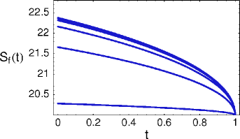
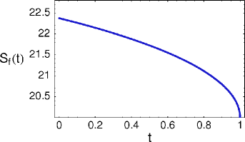
Figure 5: Five successive approximations of the free boundary $S_{f}(t)$ obtained from equation (45). The profile of the solution $S_{f}(t)$.

In Fig. 6 we show the long time behavior of the free boundary $S_{f}(t),t\in[0,T],$ for large values of the expiration time $T$. For the parameter values $T=50,r=0.1,q=0.05,\sigma=0.35$ and $E=10$ the theoretical value of $S_{f}(+\infty)$ is 36.8179 (see Dewynne et al. [16]).

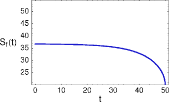
Figure 6: Long-time behavior of $S_{f}(t)$.

In Table 1 we show a comparison of results obtained by our method based on the semi-explicit formula (3.2) and those obtained by known methods based on trinomial trees (both with the depth of the tree equal to 100), finite difference approximation (with 200 spatial and time grids) and analytic approximation of Barone-Adesi & Whaley (cf. [6], [30, Ch. 15, p. 384]), resp. It also turned out that the method based on solving the integral equation (45) is 5-10 times faster than other methods based on trees or finite differences. The reason is that the computation of $V(S,t)$ for a wide range of values of $S$ based on the semi-explicit pricing formula (3.2) is very fast provided that the free boundary function $\varrho$ has already been computed.

Table 1: Comparison of the method based on formula (3.2) with other methods for the parameter values $E=10,T=1,\sigma=0.2,r=0.1,q=0.05$. The position $S_{f}(0)=\varrho(T)$ of the free boundary at $t=0$ (i.e. at $\tau=T$) was computed as $S_{f}(0)=\varrho(T)=22.3754$

Method $\backslash$   The asset value $S$	15	18	20	21	22.3754
Our method	5.15	8.09	10.03	11.01	12.37
Trinomial tree	5.15	8.09	10.03	11.01	12.37
Finite differences	5.49	8.48	10.48	11.48	12.48
Analytic approximation	5.23	8.10	10.04	11.02	12.38

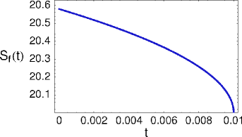
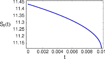
Figure 7: The early exercise boundary $S_{f}(t)$ for $r=0.1,q=0.05$. The early exercise boundary $S_{f}(t)$ for $r=0.1,q=0.09$.

In Fig. 7 the early exercise boundary $S_{f}(t)$ is computed for various values of the parameter $q$. In these computations we chose $E=10,T=0.01,\sigma=0.45$. Of interest is the case where $q$ is close to $r$ ($q=0.09$ and $r=0.1$).

3.4 Early exercise boundary for an American put option

In this section we present results of transformation method applied to valuation of the early exercise boundary for American style of a put option. Recall that the early exercise boundary problem for American put option can be formulated as follows:

$${\partial V\over\partial t}+rS{\partial V\over\partial S}+{\sigma^{2}\over 2}S^{2}{\partial^{2}V\over\partial S^{2}}-rV=0\,,\qquad 0<t<T,\ S_{f}(t)<S<\infty\,,$$

$$V(+\infty,t)=0,\ V(S_{f}(t),t)=E-S_{f}(t)\,,\ {\partial V\over\partial S}(S_{f}(t),t)=-1\,,$$ (54)

$$V(S,T)=\max(E-S,0)\,,$$

defined on a time-dependent domain $S\in(S_{f}(t),\infty)$, where $t\in(0,T)$ (cf. Kwok [38]). Again $S>0$ stands for the stock price, $E>0$ is the exercise price, $r>0$ is the risk-free rate and $\sigma>0$ is the volatility of the underlying stock process. We shall assume that the asset pay no dividends, i.e. $q=0$. In order to perform a fixed domain transformation of the free boundary problem (3.4) we introduce the following change of variables

$$x=\ln\left(\frac{S}{\varrho(\tau)}\right),\quad\hbox{where}\ \ \tau=T-t,\varrho(\tau)=S_{f}(T-\tau).$$

Similarly as in the case of a call option we define a synthetised portfolio $\Pi$ for the put option $\Pi(x,\tau)=V-S\frac{\partial V}{\partial S}$. Then it is easy to verify that $\Pi$ is a solution to the following the parabolic equation

$$\frac{\partial\Pi}{\partial\tau}-a(\tau)\frac{\partial\Pi}{\partial x}-\frac{\sigma^{2}}{2}\frac{\partial^{2}\Pi}{\partial x^{2}}+r\Pi=0,\quad x>0,\tau\in(0,T),$$

$$\Pi(0,\tau)=E,\quad\Pi(\infty,\tau)=0,$$ (55)

$$\frac{\sigma^{2}}{2}\frac{\partial\Pi}{\partial x}(0,\tau)=-rE,\quad\hbox{for}\ \tau\in(0,T),$$ (56)

$$\Pi(x,0)=0\quad\hbox{for}\quad x>0,$$

where $a(\tau)=\frac{\dot{\varrho}(\tau)}{\varrho(\tau)}+r-\frac{\sigma^{2}}{2}$ (see Stamicar et al. [50]). Now, following the same methodology of applying the Fourier transform we are able to derive an integral equation for the free boundary position. It is just the equation $\frac{\sigma^{2}}{2}\frac{\partial\Pi}{\partial x}(0,\tau)=-rE$ in which the left hand side is expressed by the inverse Fourier transform of the solution $\Pi$ as a weakly singular integral depending on the free boundary position $\varrho$ (see [50] for details). We omit the technical details here. We just recall that the integral equation for the free boundary function $\varrho(\tau)$ yields the following expression for $\varrho(\tau)$

$$\varrho(\tau)=Ee^{-(r-\frac{\sigma^{2}}{2})\tau}e^{\sigma\sqrt{2\tau}\eta(\tau)}$$

in terms of a new auxiliary function $\eta(\tau)$ (see Stamicar et al. [50] for details). Further asymptotic analysis of the integral equation enables us to derive an asymptotic formula for $\eta(\tau)$ as $\tau\to 0$. Namely,

$$\eta(\tau)\sim-\sqrt{-\ln\left[\frac{2r}{\sigma}\sqrt{2\pi\tau}e^{r\tau}\right]}\quad\hbox{as}\ \tau\to 0^{+}.$$ (57)

Figure 8: Left: asymptotic approximation vs. binomial method for $\sigma=0.25,r=0.1,E=10$ and $T-t=8.76$ hrs. (0.001 of a year), MBW approximation vs. the asymptotic solution (57) for $T-t=0.876$ hrs (right).

Next we examine how accurately our asymptotic approximation matches the data from the binomial method (cf. Kwok [38]). Near expiry at about one hour, the asymptotic approximation matches the data from the binomial method (see Fig. 8). With $\sigma=0.25,r=0.1,E=10$ at 8.76 hours the approximation gives an overestimate but of only 0.4 cents (see [50]). We also compared our asymptotic solution with MacMillan, Barone-Adesi, and Whaley’s [6], [4, 384–386], [40] numerical approximation of the American put free boundary (see Fig. 8). They apply a transformation that results in a Cauchy-Euler equation that can be solved analytically. For times very close to expiry, one can see that our approximation of the free boundary matches the data from the binomial and trinomial methods more accurately.

The numerical and analytical results obtained by the transformation method for solving free boundary problem for American put options are in agreement with those obtained recently by Zhu [55, 56], Mallier et al. [41, 42], Kuske and Keller [36], Knessl [34].

4 Transformation method for a nonlinear Black–Scholes equation

The main goal of this section is to perform a fixed domain transformation of the free boundary problem for the nonlinear Black–Scholes equation (2) into a parabolic equation defined on a fixed spatial domain. For the sake of simplicity we will present a detailed derivation of an equation only for the case of an American call option. Derivation of the corresponding equation for the American put option is similar. Throughout this section we shall assume the volatility $\sigma^{2}$ appearing in the Black–Scholes equation to be a function of the option price $S$, time to expiry $T-t$ and $S^{2}\partial^{2}_{S}V$, i.e.

$$\sigma=\sigma(S^{2}\partial^{2}_{S}V,S,T-t)\,.$$

Following (24) we shall consider the following change of variables:

$$\tau=T-t,\quad x=\ln\left(\varrho(\tau)/S\right)\ \ \hbox{where}\ \ \varrho(\tau)=S_{f}(T-\tau).$$

Then $\tau\in(0,T)$ and $x\in(0,\infty)$ iff $S\in(0,S_{f}(t))$. The boundary value $x=0$ corresponds to the free boundary position $S=S_{f}(t)$ whereas $x\approx+\infty$ corresponds to the default value $S=0$ of the underlying asset. Following Stamicar et al. [50] and Ševčovič [46, 47] we construct the so-called synthetic portfolio function $\Pi=\Pi(x,\tau)$ defined as follows:

$$\Pi(x,\tau)=V(S,t)-S\frac{\partial V}{\partial S}(S,t)\,.$$ (58)

Again, it represents a synthetic portfolio consisting of one long positioned option and $\Delta=\partial_{S}V$ underlying short stocks. Similarly as in Section 3 we have

$$\frac{\partial\Pi}{\partial x}=S^{2}\frac{\partial^{2}V}{\partial S^{2}},\ \ \frac{\partial\Pi}{\partial\tau}+\frac{\dot{\varrho}}{\varrho}\frac{\partial\Pi}{\partial x}=-\frac{\partial}{\partial t}\left(V-S\frac{\partial V}{\partial S}\right)$$

where we have denoted $\dot{\varrho}=d\varrho/d\tau$. Assuming sufficient smoothness of a solution $V=V(S,t)$ to (2) we can deduce from (2) a parabolic equation for the synthetic portfolio function $\Pi=\Pi(x,\tau)$

$$\frac{\partial\Pi}{\partial\tau}+(b(\tau)-\frac{1}{2}\sigma^{2})\frac{\partial\Pi}{\partial x}-\frac{1}{2}\frac{\partial}{\partial x}\left(\sigma^{2}\frac{\partial\Pi}{\partial x}\right)+r\Pi=0$$

defined on a fixed domain $x\in\mathbb{R},\,t\in(0,T),$ with a time-dependent coefficient

$$b(\tau)={\dot{\varrho}(\tau)\over\varrho(\tau)}+r-q$$ (59)

and a diffusion coefficient given by: $\sigma^{2}=\sigma^{2}(\partial_{x}\Pi(x,\tau),\varrho(\tau)e^{-x},\tau)$ depending on $\tau,x$ and the gradient $\partial_{x}\Pi$ of a solution $\Pi$. Now the boundary conditions $V(0,t)=0,V(S_{f}(t),t)=S_{f}(t)-E$ and $\partial_{S}V(S_{f}(t),t)=1$ imply

$$\Pi(0,\tau)=-E,\quad\Pi(+\infty,\tau)=0\,,\quad 0<\tau<T\,,$$ (60)

and, from the terminal pay-off diagram for $V(S,T)$, we deduce

$$\Pi(x,0)=\left\{\begin{array}[]{lll}-E&\hbox{for}\ x<\ln\left({\varrho(0)\over E}\right)\hfil\\ \ \ 0&\hbox{otherwise.}\hfil\end{array}\right.$$ (61)

In order to close up the system of equations that determines the value of a synthetic portfolio $\Pi$ we have to construct an equation for the free boundary position $\varrho(\tau)$. Indeed, both the coefficient $b$ as well as the initial condition $\Pi(x,0)$ depend on the function $\varrho(\tau)$. Similarly as in the case of a constant volatility $\sigma$ (see [46, 50]) we proceed as follows: since $S_{f}(t)-E=V(S_{f}(t),t)$ and $\partial_{S}V(S_{f}(t),t)=1$ we have ${\scriptstyle\frac{d}{dt}}S_{f}(t)=\partial_{S}V(S_{f}(t),t){\scriptstyle\frac{d}{dt}}S_{f}(t)+\partial_{t}V(S_{f}(t),t)$ and so $\partial_{t}V(S,t)=0$ along the free boundary $S=S_{f}(t)$. Moreover, assuming $\partial_{x}\Pi$ is continuous up to the boundary $x=0$ we obtain $S^{2}\partial^{2}_{S}V(S,t)\to\partial_{x}\Pi(0,\tau)$ and $S\partial_{S}V(S,t)\to\varrho(\tau)$ as $S\to S_{f}(t)^{-}$. Now, by taking the limit $S\to S_{f}(t)^{-}$ in the Black–Scholes equation (2) we obtain $(r-q)\varrho(\tau)+{\scriptstyle\frac{1}{2}}\sigma^{2}\partial_{x}\Pi(0,\tau)-r(\varrho(\tau)-E)=0$. Therefore

$$\varrho(\tau)={rE\over q}+\frac{1}{2q}\sigma^{2}(\partial_{x}\Pi(0,\tau),\varrho(\tau),\tau)\frac{\partial\Pi}{\partial x}(0,\tau)$$

for $0<\tau\leq T$. The value of $\varrho(0)$ can be easily derived from the smoothness assumption made on $\partial_{x}\Pi$ at the origin $x=0,\tau=0$ under the structural assumption

$$0<q<r$$ (62)

made on the interest and dividend yield rates $r,q$ (cf. [46, 47]). Indeed, continuity of $\partial_{x}\Pi$ at the origin $(0,0)$ implies $\lim_{\tau\to 0^{+}}\partial_{x}\Pi(0,\tau)=\partial_{x}\Pi(0,0)=\lim_{x\to 0^{+}}\partial_{x}\Pi(x,0)=0$ because $\Pi(x,0)=-E$ for $x$ close to $0^{+}$ provided $\ln(r/q)>0$. From the above equation for $\varrho(\tau)$ we deduce $\varrho(0)={rE\over q}$ by taking the limit $\tau\to 0^{+}$. Putting all the above equations together we end up with a closed system of equations for $\Pi=\Pi(x,\tau)$ and $\varrho=\varrho(\tau)$

$$\frac{\partial\Pi}{\partial\tau}+\bigl{(}b(\tau)-\frac{\sigma^{2}}{2}\bigr{)}\frac{\partial\Pi}{\partial x}-\frac{1}{2}\frac{\partial}{\partial x}\bigl{(}\sigma^{2}\frac{\partial\Pi}{\partial x}\bigr{)}+r\Pi=0\,,$$

$$\Pi(0,\tau)=-E\,,\ \ \Pi(+\infty,\tau)=0\,,\ x>0\,,\tau\in(0,T)\,,$$

$$\Pi(x,0)=\left\{\begin{array}[]{lll}-E&\quad\hbox{for}\ x<\ln(r/q)\hfil\\ \ \ \ 0&\quad\hbox{otherwise\,,}\hfil\end{array}\right.$$ (65)

where $\sigma=\sigma(\partial_{x}\Pi(x,\tau),\varrho(\tau)e^{-x},\tau)\,,\ b(\tau)={\dot{\varrho}(\tau)\over\varrho(\tau)}+r-q$ and the free boundary position $\varrho(\tau)=S_{f}(T-\tau)$ satisfies an implicit algebraic equation

$$\varrho(\tau)={rE\over q}+{\sigma^{2}(\partial_{x}\Pi(0,\tau),\varrho(\tau),\tau)\over 2q}\frac{\partial\Pi}{\partial x}(0,\tau)\,,\quad\hbox{with }\ \varrho(0)={rE\over q},$$ (66)

where $\tau\in(0,T)$. Notice that, in order to guarantee parabolicity of equation (65) we have to assume that the function $p\mapsto\sigma^{2}(p,\varrho(\tau)e^{-x},\tau)p$ is strictly increasing. More precisely, we shall assume that there exists a positive constant $\gamma>0$ such that

$$\sigma^{2}(p,\xi,\tau)+p\partial_{p}\sigma^{2}(p,\xi,\tau)\geq\gamma>0$$ (67)

for any $\xi>0,\tau\in(0,T)$ and $p\in\mathbb{R}$. Notice that condition (67) is satisfied for the RAPM model in which $\sigma^{2}=\hat{\sigma}^{2}(1+\mu p^{\frac{1}{3}}\xi^{-\frac{1}{3}})$ for any $\mu\geq 0$ and $p\geq 0$. Clearly $p=S^{2}\partial^{2}_{S}V>0$ for the case of plain vanilla call or put options. As far as the Barles and Soner model is concerned, we have $\sigma^{2}=\hat{\sigma}^{2}(1+\Psi(a^{2}e^{r\tau}p))$ and condition (67) is again satisfied because the function $\Psi$ is a positive and increasing function in the Barles and Soner model.

Remark 4.1

Following exactly the same argument as in (49) one can derive an explicit expression for the option price $V(S,t)$:

$$V(S,T-\tau)={S\over\varrho(\tau)}\left(\varrho(\tau)-E+\int_{0}^{\ln{\varrho(\tau)\over S}}{\rm e}^{x}\Pi(x,\tau)\,dx\right)\,.$$ (68)

4.1 An iterative algorithm for approximation of the early exercise boundary

The idea of the iterative numerical algorithm for solving the problem (65), (66) is rather simple: we use the backward Euler method of finite differences in order to discretize the parabolic equation (65) in time. In each time level we find a new approximation of a solution pair $(\Pi,\varrho)$. First we determine a new position of $\varrho$ from the algebraic equation (66). We remind ourselves that (even in the case $\sigma$ is constant) the free boundary function $\varrho(\tau)$ behaves like $rE/q+O(\tau^{1/2})$ for $\tau\to 0^{+}$ (see e.g. [16] or [46]) and so $b(\tau)=O(\tau^{-1/2})$. Hence the convective term $b(\tau)\partial_{x}\Pi$ becomes a dominant part of equation (65) for small values of $\tau$. In order to overcome this difficulty we employ the operator splitting technique for successive solving of the convective and diffusion parts of equation (65). Since the diffusion coefficient $\sigma^{2}$ depends on the derivative $\partial_{x}\Pi$ of a solution $\Pi$ itself we make several micro-iterates to find a solution of a system of nonlinear algebraic equations.

Now we present our algorithm in more details. We restrict the spatial domain $x\in(0,\infty)$ to a finite interval of values $x\in(0,L)$ where $L>0$ is sufficiently large. For practical purposes one can take $L\approx 3$ as it corresponds to the interval $S\in(S_{f}(t)e^{-L},S_{f}(t))$ in the original asset price variable $S$. The value $S_{f}(t)e^{-L}$ is then could be a good approximation for the default value $S=0$ if $L\approx 3$. Let us denote by $k>0$ the time step, $k=T/m$, and, by $h>0$ the spatial step, $h=L/n$ where $m,n\in N$ stand for the number of time and space discretization steps, resp. We denote by $\Pi_{i}^{j}$ an approximation of $\Pi(x_{i},\tau_{j})$, $\varrho^{j}\approx\varrho(\tau_{j})$, $b^{j}\approx b(\tau_{j})$ where $x_{i}=ih,\tau_{j}=jk$. We approximate the value of the volatility $\sigma$ at the node $(x_{i},\tau_{j})$ by finite difference as follows:

$$\sigma_{i}^{j}=\sigma_{i}^{j}(\varrho^{j},\Pi^{j})=\sigma((\Pi_{i+1}^{j}-\Pi_{i}^{j})/h,\varrho^{j}e^{-x_{i}},\tau_{j})\,.$$

Then for the Euler backward in time finite difference approximation of equation (65) we have

$$\frac{\Pi^{j}-\Pi^{j-1}}{k}+\left(b^{j}-\frac{1}{2}(\sigma^{j})^{2}\right)\partial_{x}\Pi^{j}-\frac{1}{2}\partial_{x}\left((\sigma^{j})^{2}\partial_{x}\Pi^{j}\right)+r\Pi^{j}=0$$ (69)

and the solution $\Pi^{j}=\Pi^{j}(x)$ is subject to Dirichlet boundary conditions at $x=0$ and $x=L$. We set $\Pi^{0}(x)=\Pi(x,0)$. Now we decompose the above problem into two parts - a convection part and a diffusive part by introducing an auxiliary intermediate step $\Pi^{j-{\scriptstyle\frac{1}{2}}}$:

(Convective part)

$$\frac{\Pi^{j-{\scriptstyle\frac{1}{2}}}-\Pi^{j-1}}{k}+b^{j}\partial_{x}\Pi^{j-{\scriptstyle\frac{1}{2}}}=0\,,$$ (70)

(Diffusive part)

$$\frac{\Pi^{j}-\Pi^{j-{\scriptstyle\frac{1}{2}}}}{k}-\frac{(\sigma^{j})^{2}}{2}\partial_{x}\Pi^{j}-\frac{1}{2}\partial_{x}\left((\sigma^{j})^{2}\partial_{x}\Pi^{j}\right)+r\Pi^{j}=0\,.$$ (71)

The idea of the operator splitting technique consists in comparison the sum of solutions to convective and diffusion part to a solution of (69). Indeed, if $\partial_{x}\Pi^{j}\approx\partial_{x}\Pi^{j-{\scriptstyle\frac{1}{2}}}$ then it is reasonable to assume that $\Pi^{j}$ computed from the system (70)–(71) is a good approximation of the system (69).

The convective part can be approximated by an explicit solution to the transport equation:

$$\partial_{\tau}\tilde{\Pi}+b(\tau)\partial_{x}\tilde{\Pi}=0\qquad\hbox{for }x>0,\ \tau\in(\tau_{j-1},\tau_{j}]$$ (72)

subject to the boundary condition $\tilde{\Pi}(0,\tau)=-E$ and initial condition $\tilde{\Pi}(x,\tau_{j-1})=\Pi^{j-1}(x)$. For American style of call option the free boundary $\varrho(\tau)=S_{f}(T-\tau)$ must be an increasing function in $\tau$ and we have assumed $0<q<r$ we have $b(\tau)=\dot{\varrho}(\tau)/\varrho(\tau)+r-q>0$ and so prescribing the in-flowing boundary condition $\tilde{\Pi}(0,\tau)=-E$ is consistent with the transport equation. Let us denote by $B(\tau)$ the primitive function to $b(\tau)$, i.e. $B(\tau)=\ln\varrho(\tau)+(r-q)\tau$. Equation (72) can be integrated to obtain its explicit solution:

$$\tilde{\Pi}(x,\tau)=\left\{\begin{matrix}\Pi^{j-1}(x-B(\tau)+B(\tau_{j-1}))\hfill&\quad\hbox{if }x-B(\tau)+B(\tau_{j-1})>0\,,\hfill\cr-E\hfill&\quad\hbox{otherwise.}\hfill\end{matrix}\right.$$ (73)

Thus the spatial approximation $\Pi^{j-{\scriptstyle\frac{1}{2}}}_{i}$ can be constructed from the formula

$$\Pi^{j-{\scriptstyle\frac{1}{2}}}_{i}=\left\{\begin{matrix}\Pi^{j-1}(\xi_{i})\hfill&\quad\hbox{if }\xi_{i}=x_{i}-\ln\varrho_{j}+\ln\varrho_{j-1}-(r-q)k>0\,,\hfill\cr-E\hfill&\quad\hbox{otherwise,}\hfill\end{matrix}\right.$$ (74)

where a linear approximation between discrete values $\Pi^{j-1}_{i},i=0,1,...,n,$ is being used to compute the value $\Pi^{j-1}(x_{i}-\ln\varrho_{j}+\ln\varrho_{j-1}-(r-q)k)$.

The diffusive part can be solved numerically by means of finite differences. Using central finite difference for approximation of the derivative $\partial_{x}\Pi^{j}$ we obtain

$$\frac{\Pi_{i}^{j}-\Pi_{i}^{j-{\scriptstyle\frac{1}{2}}}}{k}+r\Pi_{i}^{j} - \frac{(\sigma^{j}_{i})^{2}}{2}\frac{\Pi_{i+1}^{j}-\Pi_{i-1}^{j}}{2h}$$

$$- \frac{1}{2h}\left((\sigma_{i}^{j})^{2}\frac{\Pi_{i+1}^{j}-\Pi_{i}^{j}}{h}-(\sigma_{i-1}^{j})^{2}\frac{\Pi_{i}^{j}-\Pi_{i-1}^{j}}{h}\right)=0\,.$$

Hence, the vector of discrete values $\Pi^{j}=\{\Pi_{i}^{j},i=1,2,...,n\}$ at the time level $j\in\{1,2,...,m\}$ satisfies the tridiagonal system of equations

$$\alpha_{i}^{j}\Pi_{i-1}^{j}+\beta_{i}^{j}\Pi_{i}^{j}+\gamma_{i}^{j}\Pi_{i+1}^{j}=\Pi_{i}^{j-{\scriptstyle\frac{1}{2}}},$$ (75)

for $i=1,2,...,n,$ where

$$\alpha_{i}^{j} \equiv \alpha_{i}^{j}(\varrho^{j},\Pi^{j})=-\frac{k}{2h^{2}}(\sigma_{i-1}^{j})^{2}+\frac{k}{2h}\frac{(\sigma_{i}^{j})^{2}}{2},$$

$$\gamma_{i}^{j} \equiv \gamma_{i}^{j}(\varrho^{j},\Pi^{j})=-\frac{k}{2h^{2}}(\sigma_{i}^{j})^{2}-\frac{k}{2h}\frac{(\sigma_{i}^{j})^{2}}{2},$$ (76)

$$\beta_{i}^{j} \equiv \beta_{i}^{j}(\varrho^{j},\Pi^{j})=1+rk-(\alpha_{i}^{j}+\gamma_{i}^{j})\,.$$

The initial and boundary conditions at $\tau=0$ and $x=0,L,$ resp., can be approximated as follows:

$$\Pi_{i}^{0}=\left\{\begin{array}[]{lll}-E&\ \ \hbox{for}\ x_{i}<\ln\left({r/q}\right),\hfil\\ \ \ \ 0&\ \ \hbox{for}\ x_{i}\geq\ln\left({r/q}\right),\hfil\end{array}\right.$$

for $i=0,1,...,n,$ and $\Pi_{0}^{j}=-E,\quad\Pi_{n}^{j}=0$.

Next we proceed by approximation of equation (66) which introduces a nonlinear constraint condition between the early exercise boundary function $\varrho(\tau)$ and the trace of the solution $\Pi$ at the boundary $x=0$ ($S=S_{f}(t)$ in the original variable). Taking a finite difference approximation of $\partial_{x}\Pi$ at the origin $x=0$ we obtain

$$\varrho^{j}=\frac{rE}{q}+\frac{1}{2q}\sigma^{2}\left((\Pi_{1}^{j}-\Pi_{0}^{j})/h,\varrho^{j},\tau_{j}\right)\frac{\Pi_{1}^{j}-\Pi_{0}^{j}}{h}\,.$$ (77)

Now, equations (74), (75) and (77) can be written in an abstract form as a system of nonlinear equations:

$$\varrho^{j} ={\mathcal{F}}(\Pi^{j},\varrho^{j}),$$

$$\Pi^{j-{\scriptstyle\frac{1}{2}}} ={\mathcal{T}}(\Pi^{j},\varrho^{j}),$$ (78)

$${\mathcal{A}}(\Pi^{j},\varrho^{j})\Pi^{j} =\Pi^{j-{\scriptstyle\frac{1}{2}}},$$

where ${\mathcal{F}}(\Pi^{j},\varrho^{j})$ is the right-hand side of the algebraic equation (77), ${\mathcal{T}}(\Pi^{j},\varrho^{j})$ is the transport equation solver given by the right-hand side of (74) and ${\mathcal{A}}={\mathcal{A}}(\Pi^{j},\varrho^{j})$ is a tridiagonal matrix with coefficients given by (4.1). The system (78) can be approximately solved by means of successive iterates procedure. We define, for $j\geq 1,$ $\Pi^{j,0}=\Pi^{j-1},\varrho^{j,0}=\varrho^{j-1}$. Then the $(p+1)$-th approximation of $\Pi^{j}$ and $\varrho^{j}$ is obtained as a solution to the system:

$$\varrho^{j,p+1} ={\mathcal{F}}(\Pi^{j,p},\varrho^{j,p}),$$

$$\Pi^{j-{\scriptstyle\frac{1}{2}},p+1} ={\mathcal{T}}(\Pi^{j,p},\varrho^{j,p+1}),$$ (79)

$${\mathcal{A}}(\Pi^{j,p},\varrho^{j,p+1})\Pi^{j,p+1} =\Pi^{j-{\scriptstyle\frac{1}{2}},p+1}\,.$$

Notice that the last equation is a linear tridiagonal equation for the vector $\Pi^{j,p+1}$ whereas $\varrho^{j,p+1}$ and $\Pi^{j-{\scriptstyle\frac{1}{2}},p+1}$ can be directly computed from (77) and (74), resp. If the sequence of approximate solutions $\{(\Pi^{j,p},\varrho^{j,p})\}_{p=1}^{\infty}$ converges to some limiting value $(\Pi^{j,\infty},\varrho^{j,\infty})$ as $p\to\infty$ then this limit is a solution to a nonlinear system of equations (78) at the time level $j$ and we can proceed by computing the approximate solution the next time level $j+1$.

4.2 Numerical approximations of the early exercise boundary

In this section we focus on numerical experiments based on the iterative scheme described in the previous section. The main purpose is to compute the free boundary profile $S_{f}(t)=\varrho(T-t)$ for different (non)linear Black–Scholes models and for various model parameters. A solution $(\Pi,\varrho)$ has been computed by our iterative algorithm for the following basic model parameters: $E=10,T=1$ (one year), $r=0.1$ (10% p.a) , $q=0.05$ (5% p.a.) and $\hat{\sigma}=0.2$. We used $n=750$ spatial points and $m=225000$ time discretization steps. Such a time step $k=T/m$ corresponds to 140 seconds between consecutive time levels when expressed in real time scale. In average we needed $p\leq 6$ micro-iterates (79) in order to solve the nonlinear system (78) with the precision $10^{-7}$.

4.2.1 Case of a constant volatility – comparison study

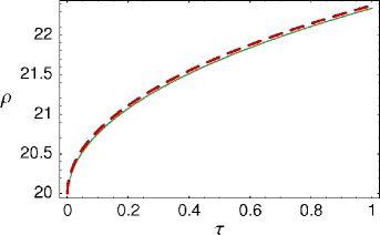
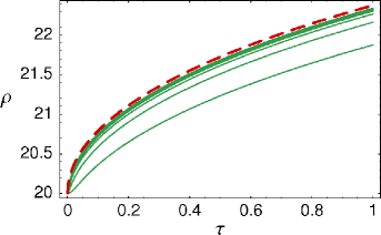
a)                                                      b)

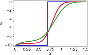
c)

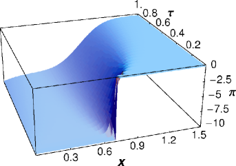
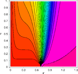
d)                                                      e)

Figure 9: a) A comparison of the free boundary function $\varrho(\tau)$ computed by the iterative algorithm (green solid curve) to the integral equation based approximation (dashed red curve); b) free boundary positions computed for various mesh sizes; c) a solution profile $\Pi(x,\tau)$ for $\tau=0$ (blue line), $\tau=T/2$ (red curve), $\tau=T$ (green curve); d) 3D plot and e) contour plot of the function $\Pi(x,\tau)$.

In our first numerical experiment we make attempt to compare our iterative approximation scheme for solving the free boundary problem for an American call option to known schemes in the case when the volatility $\sigma>0$ is constant. We compare our solution to the one computed by means of a solution to a nonlinear integral equation for $\varrho(\tau)$ (see also [46, 50]). This comparison can be also considered as a benchmark or test example for which we know a solution that can be computed by a another justified algorithm. In Fig. 9, part a), we show the function $\varrho$ computed by our iterative algorithm for $E=10,T=1,r=0.1,q=0.05,\sigma=0.2$. At the expiry $T=1$ the value of $\varrho(T)$ was computed as: $\varrho(T)=22.321$. The corresponding value $\varrho(T)$ computed from the integral equation (3.2) (cf. [46]) was $\varrho(T)=22.375$. The relative error is less than 0.25%. In the part b) we present 7 approximations of the free boundary function $\varrho(\tau)$ computed for different mesh sizes $h$ (see Tab. 2 for details). The sequence of approximate free boundaries $\varrho_{h},h=h_{1},h_{2},...,$ converges monotonically from below to the free boundary function $\varrho$ as $h\downarrow 0$. The next part c) of Fig. 9 depicts various solution profiles of a function $\Pi(x,\tau)$. In order to achieve a reasonable approximation to equation (77) we need very accurate approximation of $\Pi(x,\tau)$ for $x$ close to the origin $0$. The parts d) and e) of Fig. 9 depict the contour and 3D plots of the function $\Pi(x,\tau)$.

In Tab. 2 we present the numerical error analysis for the distance $\|\varrho_{h}-\varrho\|_{p}$ measured in two different norms ($L^{\infty}$ and $L^{2}$) of a computed free boundary position $\varrho_{h}$ corresponding to the mesh size $h$ and the solution $\varrho$ computed from the integral equation described in (3.2) (cf. [46]). The time step $k$ has been adjusted to the spatial mesh size $h$ in order to satisfy CFL condition $\hat{\sigma}^{2}k/h^{2}\approx 1/2$. We also computed the experimental order of convergence $\hbox{eoc}(L^{p})$ for $p=2,\infty$. Recall that the experimental order of convergence can be defined as the ratio:

$$\hbox{eoc}(L^{p})=\frac{\ln(\|\varrho_{h_{i}}-\varrho\|_{p})-\ln(\|\varrho_{h_{i-1}}-\varrho\|_{p})}{\ln h_{i}-\ln h_{i-1}}\,.$$

It can be interpreted as an exponent $\alpha=\hbox{eoc}(L^{p})$ for which we have $\|\varrho_{h}-\varrho\|_{p}=O(h^{\alpha})$. It turns out from Tab. 2 that the conjecture on the order of convergence $\|\varrho_{h}-\varrho\|_{\infty}=O(h)$ whereas $\|\varrho_{h}-\varrho\|_{2}=O(h^{3/2})$ as $h\to 0^{+}$ could be reasonable.

Table 2: Experimental order of convergence of the iterative algorithm for approximating the free boundary position.

$h$	err($L^{\infty}$)	eoc($L^{\infty}$)	err($L^{2}$)	eoc($L^{2}$)
0.03	0.5	-	0.808	-
0.012	0.215	0.92	0.227	1.39
0.006	0.111	0.96	0.0836	1.44
0.004	0.0747	0.97	0.0462	1.46
0.003	0.0563	0.98	0.0303	1.47
0.0024	0.0452	0.98	0.0218	1.48
0.002	0.0378	0.98	0.0166	1.48

4.2.2 Risk Adjusted Pricing Methodology model

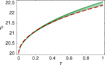
Figure 10: A comparison of the free boundary function $\varrho^{R}(\tau)$ computed for the Risk Adjusted Pricing Methodology model. Dashed red curve represents a solution corresponding to $R=0$, whereas the green curves represent a solution $\varrho^{R}(\tau)$ for different values of the risk premium coefficients $R=5,15,40,70,100$.

In the next example we computed the position of the free boundary $\varrho(\tau)$ in the case of the Risk Adjusted Pricing Methodology model - a nonlinear Black–Scholes type model derived by Jandačka and Ševčovič in [32]. In this model the volatility $\sigma$ is a nonlinear function of the asset price $S$ and the second derivative $\partial_{S}^{2}V$ of the option price, and it is given by formula (8). In Fig. 10 we present results of numerical approximation of the free boundary position $\varrho^{R}(\tau)=S_{f}^{R}(T-\tau)$ in the case when the coefficient of transaction costs $C=0.01$ is fixed and the risk premium measure $R$ varies from $R=5,15,40,70,$ up to $R=100$. We compare the position of the free boundary $\varrho^{R}(\tau)$ to the case when there are no transaction costs and no risk from volatile portfolio, i.e. we compare it with the free boundary position $\varrho^{0}(\tau)$ for the linear Black–Scholes equation (see Fig. 10). An increase in the risk premium coefficient $R$ resulted in an increase of the free boundary position as it can be expected.

Table 3: Distance $\|\varrho^{R}-\varrho^{0}\|_{p}$ ($p=2,\infty$) of the free boundary position $\varrho^{R}$ from the reference free boundary position $\varrho^{0}$ and experimental orders $\alpha_{\infty}$ and $\alpha_{2}$ of convergence.

$R$	$\|\varrho^{R}-\varrho^{0}\|_{\infty}$	$\alpha_{\infty}$	$\|\varrho^{R}-\varrho^{0}\|_{2}$	$\alpha_{2}$
1	0.0601	-	0.0241	-
2	0.0754	0.33	0.0303	0.328
5	0.102	0.33	0.0408	0.326
10	0.128	0.33	0.0511	0.324
15	0.145	0.32	0.0582	0.323
20	0.16	0.32	0.0639	0.322
30	0.182	0.32	0.0727	0.321
40	0.2	0.32	0.0798	0.32
50	0.214	0.32	0.0856	0.319
60	0.227	0.32	0.0907	0.318
70	0.239	0.32	0.0953	0.317
80	0.249	0.32	0.0994	0.317
90	0.259	0.32	0.103	0.316
100	0.268	0.32	0.107	0.316

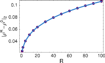
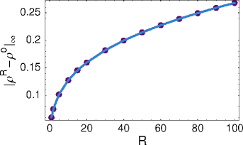
Figure 11: Dependence of the norms $\|\varrho^{R}-\varrho^{0}\|_{p}$ ($p=\infty,2$) of the deviation of the free boundary $\varrho=\varrho^{R}(\tau)$ for the RAPM model on the risk premium coefficient $R$.

In Tab. 3 and Fig. 10 we summarize results of comparison of the free boundary position $\varrho^{R}$ for various values of the risk premium coefficient to the reference position $\varrho=\varrho^{0}$ computed from the Black–Scholes model with a constant volatility $\sigma=\hat{\sigma}$, i.e. $R=0$. The experimental order $\alpha_{p}$ of the distance function $\|\varrho^{R}-\varrho^{0}\|_{p}=O(R^{\alpha_{p}})$ has been computed for $p=2,\infty$, as follows:

$$\alpha_{p}=\frac{\ln(\|\varrho^{R_{i}}-\varrho^{0}\|_{p})-\ln(\|\varrho^{R_{i-1}}-\varrho^{0}\|_{p})}{\ln R_{i}-\ln R_{i-1}}\,.$$

According to the values presented in Tab. 3 it turns out that a reasonable conjecture on the order of convergence is that $\|\varrho^{R}-\varrho^{0}\|_{p}=O(R^{1/3})$ for both norms $p=2$ and $p=\infty$. Since the transaction cost coefficient $C$ and risk premium measure $R$ enter the expression for the RAPM volatility (8) only in the product $C^{2}R$ we can conjecture that $\|\varrho^{R,C}-\varrho^{0,0}\|_{p}=O(C^{2/3}R^{1/3})$ as either $C\to 0^{+}$ or $R\to 0^{+}$.

4.2.3 Barles and Soner model

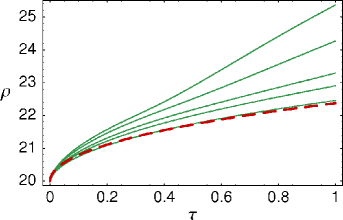
Figure 12: A comparison of the free boundary function $\varrho(\tau)$ computed for the Barles and Soner model. Dashed red curve represents a solution corresponding to $R=0$, whereas the green curves represents a solution $\varrho(\tau)$ for different values of the risk aversion coefficient $a=0.01,0.07,0.13,0.25,0.35$.

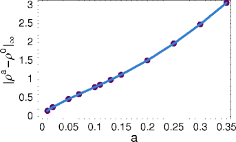
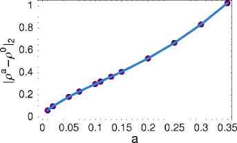
Figure 13: Dependence of the norms $\|\varrho^{a}-\varrho^{0}\|_{p}$ ($p=\infty,2$) of the deviation of the free boundary $\varrho=\varrho^{a}(\tau)$ for the Barles-Soner model on the risk aversion parameter $a$.

Table 4: Distance $\|\varrho^{a}-\varrho^{0}\|_{p}$ ($p=2,\infty$) of the free boundary position $\varrho^{a}$ from the reference free boundary position $\varrho^{0}$ and experimental orders $\alpha_{\infty}$ and $\alpha_{2}$ of convergence.

$a$	$\|\varrho^{a}-\varrho^{0}\|_{\infty}$	$\alpha_{\infty}$	$\|\varrho^{a}-\varrho^{0}\|_{2}$	$\alpha_{2}$
0.01	0.156	-	0.0615	-
0.02	0.25	0.68	0.0985	0.68
0.05	0.472	0.69	0.184	0.679
0.07	0.602	0.72	0.232	0.69
0.1	0.793	0.77	0.298	0.712
0.11	0.857	0.82	0.32	0.74
0.13	0.99	0.86	0.364	0.766
0.15	1.13	0.92	0.409	0.807
0.2	1.52	1.	0.529	0.897
0.25	1.97	1.2	0.669	1.05
0.3	2.49	1.3	0.833	1.21
0.35	3.07	1.4	1.03	1.35

Our next example is devoted to the nonlinear Black–Scholes model due to Barles and Soner (see [8]). In this model the volatility is given by equation (6). Numerical results are depicted in Fig. 12. Choosing a larger value of the risk aversion coefficient $a>0$ resulted in increase of the free boundary position $\varrho^{a}(\tau)$. The position of the early exercise boundary $\varrho^{a}(\tau)$ has considerably increased in comparison to the linear Black–Scholes equation with constant volatility $\sigma=\hat{\sigma}$. In contrast to the case of constant volatility as well as the RAPM model, there is, at least a numerical evidence (see Fig.12 and $\varrho^{a}$ for the largest value $a=0.35$) that the free boundary profile $\varrho^{a}(\tau)$ need not be necessarily convex. Recall that that convexity of the free boundary profile has been proved analytically by Ekström et al. and Chen et al. in a recent papers [13, 20, 19] in the case of a American put option and constant volatility $\sigma=\hat{\sigma}$.

Similarly as in the previous model we also investigated the dependence of the free boundary position $\varrho=\varrho^{a}(\tau)$ on the risk aversion parameter $a>0$. In Tab. 4 and Fig. 13 we present results of comparison of the free boundary position $\varrho^{a}$ for various values of the risk aversion coefficient $a$ to the reference position $\varrho=\varrho^{0}$. Inspecting values $\alpha_{p}$ of the order of distance $\|\varrho^{a}-\varrho^{0}\|_{p}$ it can be conjectured that $\|\varrho^{a}-\varrho^{0}\|_{p}=O(a^{2/3})$ as $a\to 0$ for both norms $p=2$ and $p=\infty$.

5 Transformation methods for Asian call options

Path dependent options are options whose pay-off diagram depends on the path history of the underlying asset. Among path dependent options Asian options plays an important role as they are quite common in currency and commodity markets like e.g. oil industry (cf. [28, 15]). Asian options may depend on the averaged path history in several ways. We shall restrict our attention to the so-called floating strike Asian call options. The floating strike price is assumed to be an arithmetic average of the underlying asset prices over the entire time interval $[0,T]$ where $T$ is the expiration time.

Let us define the arithmetic average $A=A_{t}$ of the underlying asset $S=S_{t}$ by

$$A_{t}=\frac{1}{t}\int_{0}^{t}S_{\tau}\,d\tau\,.$$

For the case of the so-called Asian floating strike call option the pay-off diagram at expiry $T$ reads as follows: $V(S,A,T)=\max(S-A,0)$. It means the price $V$ of an option contract will depend not only on the underlying asset price $S$, time $t,$ but also on the underlying asset path average $A$, i.e. $V=V(S,A,t)$.

5.1 Governing equations for Asian options

As it is usual in the option pricing theory, we shall describe the asset price dynamics by a geometric Brownian with drift $\varrho$, dividend yield $q\geq 0$ and volatility $\sigma$, i.e. $dS=(\varrho-q)Sdt+\sigma SdW$ where $W$ is the standard Wiener process. If we apply Itô’s formula to the function $V=V(S,A,t)$ we obtain

$$dV=\left(\frac{\partial V}{\partial t}+\frac{\sigma^{2}}{2}S^{2}\frac{\partial^{2}V}{\partial S^{2}}\right)+\frac{\partial V}{\partial S}dS+\frac{\partial V}{\partial A}dA\,.$$

In the case of arithmetic averaging we have $dA=t^{-1}(S-A)dt$. Hence the differential $dA$ is of the order of $dt$ and this is why the above expression for $dV$ indeed represents its lowest order approximation when taking into account stochastic character of the dynamics of the asset price $S$. Therefore, following standard arguments from the Black–Scholes theory one can derive the governing equation for pricing Asian option with arithmetic averaging in the form:

$$\frac{\partial V}{\partial t}+\frac{\sigma^{2}}{2}S^{2}\frac{\partial^{2}V}{\partial S^{2}}+S(r-q)\frac{\partial V}{\partial S}+\frac{S-A}{t}\frac{\partial V}{\partial A}-rV=0,$$ (80)

where $0<t<T,\ S,A>0$ (see e.g. [15]). For Asian call option the above equation is subject to the terminal pay-off condition

$$V(S,A,T)=\max(S-A,0),\quad S,A>0\,.$$ (81)

It is well known (see e.g. [38, 15]) that for Asian options with floating strike we can achieve dimension reduction by introducing the following similarity variable:

$$x=\frac{S}{A},\qquad W(x,\tau)=\frac{1}{A}V(S,A,t)$$

where $\tau=T-t$. It is straightforward to verify that $V(S,A,t)=W(S/A,T-t)A$ is a solution of (80) iff $W=W(x,\tau)$ is a solution to the following parabolic PDE:

$$\frac{\partial W}{\partial\tau}-\frac{\sigma^{2}}{2}x^{2}\frac{\partial^{2}W}{\partial x^{2}}-(r-q)x\frac{\partial W}{\partial x}-\frac{x-1}{T-\tau}\left(W-x\frac{\partial W}{\partial x}\right)+rW=0,$$ (82)

where $x>0$ and $0<\tau<T$. The initial condition for $W$ immediately follows from the terminal pay-off diagram for the call option,

$$W(x,0)=\max(x-1,0).$$ (83)

5.2 American style of Asian options

Following Dai and Kwok [15], American style of Asian options is characterized by the exercise region

$${\mathcal{E}}=\{(S,A,t)\in[0,\infty)\times[0,\infty)\times[0,T),\ V(S,A,t)=V(S,A,T)\}.$$

In the case of a call option this region can be described by an early exercise boundary function $S_{f}=S_{f}(A,t)$ such that

$${\mathcal{E}}=\{(S,A,t)\in[0,\infty)\times[0,\infty)\times[0,T),\ S\geq S_{f}(A,t)\}.$$

For American style of an Asian call option we have to impose a homogeneous Dirichlet boundary condition $V(0,A,t)=0$ at $S=0$. According to [15] the $C^{1}$ continuity condition at the point $(S_{f}(A,t),A,t)$ of a contact of a solution $V$ with its pay-off diagram implies the following boundary condition at the free boundary position $S_{f}(A,t)$:

$$\frac{\partial V}{\partial S}(S_{f}(A,t),A,t)=1,\quad V(S_{f}(A,t),A,t)=S_{f}(A,t)-A$$ (84)

for any $A>0$ and $0<t<T$. It is important to emphasize that the free boundary function $S_{f}$ can be also reduced to a function of one variable by introducing a new state function $x_{f}(t)$ as follows:

$$S_{f}(A,t)=Ax_{f}(t).$$

The function $x_{f}=x_{f}(t)$ is a free boundary function for the transformed state variable $x=S/A$. For American style of Asian call options the spatial domain for the reduced equation (82) is given by

$$0<x<\varrho(\tau),\ \ \tau\in(0,T),\quad\hbox{where}\ \varrho(\tau)=x_{f}(T-\tau)\,.$$

Taking into account boundary conditions (84) for the option price $V$ we end up with corresponding boundary conditions for the function $W$:

$$W(0,\tau)=0,\qquad W(x,\tau)=x-1,\ \ \frac{\partial W}{\partial x}(x,\tau)=1\ \ \hbox{at}\ \ x=\varrho(\tau)$$ (85)

for any $0<\tau<T$ and the initial condition

$$W(x,0)=\max(x-1,0)$$ (86)

for any $x>0$.

5.3 Fixed domain transformation for American style of Asian call options

Similarly as in Section 3, in order to apply the fixed domain transformation for the free boundary problem (82), (85), (86) we introduce a new variable $\xi$ and an auxiliary function $\Pi=\Pi(\xi,\tau)$ (again representing a synthetic portfolio) defined as follows:

$$\xi=\ln\left(\frac{\varrho(\tau)}{x}\right),\qquad\Pi(\xi,\tau)=W(x,\tau)-x\frac{\partial W}{\partial x}\,.$$ (87)

Clearly, $x\in(0,\varrho(\tau))$ iff $\xi\in(0,\infty)$ for $\tau\in(0,T)$. The value $\xi=\infty$ of the transformed variable corresponds to the value $x=0$ ($S=0$) expressed in the original variable. On the other hand, the value $\xi=0$ corresponds to the free boundary position $x=\varrho(\tau)$ ($S=AS_{f}(A,t)$).

A straightforward calculation similar to that of Section 4 enables us to to justify that the function $\Pi=\Pi(\xi,\tau)$ is a solution to the following parabolic PDE

$$\frac{\partial\Pi}{\partial\tau}+a(\xi,\tau)\frac{\partial\Pi}{\partial\xi}-\frac{\sigma^{2}}{2}\frac{\partial^{2}\Pi}{\partial\xi^{2}}+\left(r+\frac{1}{T-\tau}\right)\Pi=0,$$ (88)

where the term $a(\xi,\tau)$ is given by

$$a(\xi,\tau)=\frac{\dot{\rho}(\tau)}{\rho(\tau)}+r-q-\frac{\sigma^{2}}{2}-\frac{\rho e^{-\xi}-1}{T-\tau}.$$ (89)

Notice the spatial dependence of the coefficient $a=a(\xi,\tau)$ in comparison to the case of transformed equations for a linear or nonlinear Black–Scholes equations (see (3.1), (59)). The initial condition for the solution $\Pi$ follows from (86)

$$\Pi(\xi,0)=\left\{\begin{array}[]{ll}-1&\mbox{$\xi<\ln\rho(0)$},\\ 0&\mbox{$\xi>\ln\rho(0)$}.\end{array}\right.$$

Since $\partial_{x}W(x,\tau)=1$ for $x=\varrho(\tau)$ and $W(0,\tau)=0$ we conclude the Dirichlet boundary conditions for the function $\Pi$

$$\Pi(0,\tau)=-1,\qquad\Pi(\infty,\tau)=0.$$

It remains to determine an algebraic constraint between the free boundary function $\varrho(\tau)$ and the solution $\Pi$. Similarly as in the case of a linear or nonlinear Black–Scholes equation we obtain, by differentiation the condition $W(\rho(\tau),\tau)=\rho(\tau)-1$ with respect to $\tau,$ the following identity:

$$\frac{d}{d\tau}\rho(\tau)=\frac{\partial W}{\partial x}(\rho(\tau),\tau)\frac{d}{d\tau}\rho(\tau)+\frac{\partial W}{\partial\tau}(\rho(\tau),\tau).$$

Since $\frac{\partial W}{\partial x}(\rho(\tau),\tau)=1$ we have $\frac{\partial W}{\partial\tau}(x,\tau)=0$ at $x=\varrho(\tau)$. Assuming continuity of the function $\Pi$ and its derivative $\Pi_{\xi}$ up to the boundary $\xi=0$ we have

$$x^{2}\frac{\partial^{2}W}{\partial x^{2}}(x,\tau)\to\frac{\partial\Pi}{\partial\xi}(0,\tau),\quad x\frac{\partial W}{\partial x}(x,\tau)\to\rho(\tau)$$

as $x\to\rho(\tau)$. Passing to the limit $x\to\rho(\tau)$ in equation (82) we end up with the equation

$$-(r-q)\rho(\tau)-\frac{\sigma^{2}}{2}\frac{\partial\Pi}{\partial\xi}(0,\tau)+\frac{\rho(\tau)-1}{T-\tau}+r[\rho(\tau)-1]=0.$$

It yields an algebraic nonlocal expression for the free boundary position $\varrho(\tau)$

$$\rho(\tau)=\frac{r+\frac{1}{T-\tau}+\frac{\sigma^{2}}{2}\frac{\partial\Pi}{\partial\xi}(0,\tau)}{q+\frac{1}{T-\tau}}.$$ (90)

Next we determine the starting point of the free boundary function $\varrho(0)$. It means that we have to find the terminal value of the original state variable $x_{f}(T)$. We shall assume a structural assumption

$$r>q\geq 0$$ (91)

on the interest and dividend rates $r,q$. If $\varrho(0)>1$ then $\ln\varrho(0)>0$ and this is why the initial function $\Pi(\xi,0)$ is equal to $-1$ in some right neighborhood of $\xi=0$. Thus $\partial_{\xi}\Pi(\xi,0)=0$ for $0<\xi\ll 1$. Again, assuming continuity of $\partial_{\xi}\Pi(\xi,\tau)$ at $(\xi,\tau)=(0,0)$ we obtain

$$\lim_{\tau\rightarrow 0^{+}}\frac{\partial\Pi}{\partial\xi}(0,\tau)=\lim_{\tau\rightarrow 0^{+},x\rightarrow 0^{+}}\frac{\partial\Pi}{\partial\xi}(x,\tau)=\lim_{x\rightarrow 0^{+}}\frac{\partial\Pi}{\partial\xi}(x,0)=0.$$

As a consequence we can conclude

$$\rho(0)=\frac{r+\frac{1}{T}}{q+\frac{1}{T}}=\frac{1+rT}{1+qT}>1.$$

This initial condition for $\varrho(0)$ is exactly the same as the one derived recently by Dai and Kwok in [15]. They proved, for a general choice of $r,q\geq 0$ that the initial condition for the function $\varrho$ is given by

$$\varrho(0)=\max\left(\frac{1+rT}{1+qT},1\right).$$

In summary, we have transformed the free boundary problem for pricing American style of Asian call option with floating strike price into the following nonlocal parabolic PDE with an algebraic constraint

$$\frac{\partial\Pi}{\partial\tau}+a(\xi,\tau)\frac{\partial\Pi}{\partial\xi}-\frac{\sigma^{2}}{2}\frac{\partial^{2}\Pi}{\partial\xi^{2}}+\left(r+\frac{1}{T-\tau}\right)\Pi=0,\quad 0<\tau<T,\ \xi>0,$$

$$\rho(\tau)=\frac{1+r(T-\tau)+\frac{\sigma^{2}}{2}(T-\tau)\frac{\partial\Pi}{\partial\xi}(0,\tau)}{1+q(T-\tau)},\ \ 0<\tau<T,$$

subject to initial and boundary conditions

$$\Pi(0,\tau)=-1,\qquad\Pi(\infty,\tau)=0,$$

$$\Pi(\xi,0)=\left\{\begin{array}[]{ll}-1&\mbox{$\xi<\ln((1+rT)/(1+qT))$},\\ 0&\mbox{$\xi>\ln((1+rT)/(1+qT))$},\end{array}\right.$$ (94)

$$\varrho(0)=(1+rT)/(1+qT),$$

where

$$a(\xi,\tau)=\frac{\dot{\rho}(\tau)}{\rho(\tau)}+r-q-\frac{\sigma^{2}}{2}-\frac{\rho e^{-\xi}-1}{T-\tau}.$$

5.4 An approximation scheme for pricing American style of Asian options

Similarly as in the case of a nonlinear Black–Scholes equation (see Section 4) we restrict the spatial domain $\xi\in(0,\infty)$ to a finite interval of values $\xi\in(0,L)$ where $L>0$ is sufficiently large. Let $k>0$ denote by the time step, $k=T/m$, and, by $h>0$ the spatial step, $h=L/n$ where $m,n\in N$ again stand for the number of time and space discretization steps, resp. We denote by $\Pi_{i}^{j}$ an approximation of $\Pi(\xi_{i},\tau_{j})$, $\varrho^{j}\approx\varrho(\tau_{j})$ where $\xi_{i}=ih$ and $\tau_{j}=jk$. Then for the Euler backward in time finite difference approximation of equation (65) we have

$$\frac{\Pi^{j}-\Pi^{j-1}}{k}+b^{j}\frac{\partial\Pi^{j}}{\partial\xi}-\left(\frac{\sigma^{2}}{2}+\frac{\rho^{j}e^{-\xi}-1}{T-\tau_{j}}\right)\frac{\partial\Pi^{j}}{\partial\xi}-\frac{\sigma^{2}}{2}\frac{\partial^{2}\Pi^{j}}{\partial^{2}\xi}+\left(r+\frac{1}{T-\tau_{j}}\right)\Pi^{j}=0$$ (95)

where $b^{j}$ is an approximation of the value $b(\tau_{j})$ where the function $b(\tau)$ is defined as in (59), i.e. $b(\tau)={\dot{\varrho}(\tau)\over\varrho(\tau)}+r-q$. The solution $\Pi^{j}=\Pi^{j}(x)$ is subject to Dirichlet boundary conditions at $\xi=0$ and $\xi=L$. We set $\Pi^{0}(\xi)=\Pi(\xi,0)$ (see (5.3). Again we split the above problem into a convection part and a diffusive part by introducing an auxiliary intermediate step $\Pi^{j-{\scriptstyle\frac{1}{2}}}$:

(Convective part)

$$\frac{\Pi^{j-{\scriptstyle\frac{1}{2}}}-\Pi^{j-1}}{k}+b^{j}\partial_{x}\Pi^{j-{\scriptstyle\frac{1}{2}}}=0\,,$$ (96)

(Diffusive part)

$$\frac{\Pi^{j}-\Pi^{j-{\scriptstyle\frac{1}{2}}}}{k}-\left(\frac{\sigma^{2}}{2}+\frac{\rho^{j}e^{-\xi}-1}{T-\tau_{j}}\right)\frac{\partial\Pi^{j}}{\partial\xi}-\frac{\sigma^{2}}{2}\frac{\partial^{2}\Pi^{j}}{\partial^{2}\xi}+\left(r+\frac{1}{T-\tau_{j}}\right)\Pi^{j}=0.$$ (97)

The convective part can be approximated by an explicit solution to the transport equation $\partial_{\tau}\tilde{\Pi}+b(\tau)\partial_{\xi}\tilde{\Pi}=0$ for $\xi>0$ and $\tau\in(\tau_{j-1},\tau_{j}]$ subject to the boundary condition $\tilde{\Pi}(0,\tau)=-1$ and the initial condition $\tilde{\Pi}(\xi,\tau_{j-1})=\Pi^{j-1}(\xi)$. In contrast to classical plain vanilla call or put options the free boundary function $\varrho(\tau)$ need not be monotonically increasing (see e.g. [15] or [28]). Therefore depending on whether the term $b(\tau)={\dot{\varrho}(\tau)\over\varrho(\tau)}+r-q$ is positive or negative the boundary condition $\tilde{\Pi}(0,\tau)=-1$ at $\xi=0$ is either in-flowing ($b>0$) or out-flowing ($b<0$). It means that the boundary condition $\Pi(0,\tau)=-1$ can be prescribed only if $b(\tau)\geq 0$. Let us denote by $B(\tau)$ the primitive function to $b(\tau)$, i.e. $B(\tau)=\ln\varrho(\tau)+(r-q)\tau$. Solving the equation $\partial_{\tau}\tilde{\Pi}+b(\tau)\partial_{\xi}\tilde{\Pi}=0$ we obtain: $\tilde{\Pi}(\xi,\tau)=\Pi^{j-1}(\xi-B(\tau)+B(\tau_{j-1}))$ if $\xi-B(\tau)+B(\tau_{j-1})>0$ and $\tilde{\Pi}(\xi,\tau)=-1$ otherwise. Hence the full time-space approximation of the half-step solution $\Pi^{j-{\scriptstyle\frac{1}{2}}}_{i}$ can be obtained from the formula

$$\Pi^{j-{\scriptstyle\frac{1}{2}}}_{i}=\left\{\begin{matrix}\Pi^{j-1}(\eta_{i})\hfill&\quad\hbox{if }\eta_{i}=\xi_{i}-\ln\varrho_{j}+\ln\varrho_{j-1}-(r-q)k>0\,,\hfill\cr-1\hfill&\quad\hbox{otherwise.}\hfill\end{matrix}\right.$$ (98)

In order to compute the value $\Pi^{j-1}(\eta_{i})$ we make use of a linear approximation between discrete values $\Pi^{j-1}_{i},i=0,1,...,n$.

Using central finite differences for approximation of the derivative $\partial_{x}\Pi^{j}$ we can approximate the diffusive part of a solution (97) as follows:

$$\frac{\Pi_{i}^{j}-\Pi_{i}^{j-{\scriptstyle\frac{1}{2}}}}{k} + \left(r+\frac{1}{T-\tau_{j}}\right)\Pi_{i}^{j}$$

$$- \left(\frac{\sigma^{2}}{2}+\frac{\rho^{j}e^{-\xi_{i}}-1}{T-\tau_{j}}\right)\frac{\Pi_{i+1}^{j}-\Pi_{i-1}^{j}}{2h}-\frac{\sigma^{2}}{2}\frac{\Pi_{i+1}^{j}-2\Pi_{i}^{j}+\Pi_{i-1}^{j}}{h^{2}}=0\,.$$

Therefore the vector of discrete values $\Pi^{j}=\{\Pi_{i}^{j},i=1,2,...,n\}$ at the time level $j\in\{1,2,...,m\}$ is a solution to a tridiagonal system of equations

$$\alpha_{i}^{j}\Pi_{i-1}^{j}+\beta_{i}^{j}\Pi_{i}^{j}+\gamma_{i}^{j}\Pi_{i+1}^{j}=\Pi_{i}^{j-{\scriptstyle\frac{1}{2}}}$$ (100)

for $i=1,2,...,n,$ where

$$\alpha_{i}^{j} \equiv \alpha_{i}^{j}(\varrho^{j})=-\frac{k}{2h^{2}}\sigma^{2}+\frac{k}{2h}\left(\frac{\sigma^{2}}{2}+\frac{\rho^{j}e^{-\xi_{i}}-1}{T-\tau_{j}}\right),$$

$$\gamma_{i}^{j} \equiv \gamma_{i}^{j}(\varrho^{j})=-\frac{k}{2h^{2}}\sigma^{2}-\frac{k}{2h}\left(\frac{\sigma^{2}}{2}+\frac{\rho^{j}e^{-\xi_{i}}-1}{T-\tau_{j}}\right),$$ (101)

$$\beta_{i}^{j} \equiv \beta_{i}^{j}(\varrho^{j})=1+\left(r+\frac{1}{T-\tau_{j}}\right)k-(\alpha_{i}^{j}+\gamma_{i}^{j})\,.$$

The initial and boundary conditions at $\tau=0$ and $x=0,L,$ can be approximated as follows:

$$\Pi_{i}^{0}=\left\{\begin{array}[]{lll}-1&\ \ \hbox{for}\ \xi_{i}<\ln\left((1+rT)/(1+qT)\right),\hfil\\ \ \ \ 0&\ \ \hbox{for}\ \xi_{i}\geq\ln\left({(1+rT)/(1+qT)}\right),\hfil\end{array}\right.$$

for $i=0,1,...,n,$ and $\Pi_{0}^{j}=-E,\quad\Pi_{n}^{j}=0$. The equation for the free boundary position $\varrho$ can be approximated by means of a finite difference approximation of $\partial_{x}\Pi$ at the origin $\xi=0$ as follows:

$$\varrho^{j}=\frac{1+r(T-\tau_{j})+(T-\tau_{j})\frac{\sigma^{2}}{2}\frac{\Pi_{1}^{j}-\Pi_{0}^{j}}{h}}{1+q(T-\tau_{j})}.$$ (102)

We formally rewrite discrete equations (98), (100) and (102) in the operator form:

$$\varrho^{j} ={\mathcal{F}}(\Pi^{j}),$$

$$\Pi^{j-{\scriptstyle\frac{1}{2}}} ={\mathcal{T}}(\Pi^{j},\varrho^{j}),$$ (103)

$${\mathcal{A}}(\varrho^{j})\Pi^{j} =\Pi^{j-{\scriptstyle\frac{1}{2}}},$$

where ${\mathcal{F}}(\Pi^{j})$ is the right-hand side of the algebraic equation (102), ${\mathcal{T}}(\Pi^{j},\varrho^{j})$ is the transport equation solver given by the right-hand side of (98) and ${\mathcal{A}}={\mathcal{A}}(\varrho^{j})$ is a tridiagonal matrix with coefficients given by (5.4). The system (103) can be approximately solved by means of successive iterates procedure. We define, for $j\geq 1,$ $\Pi^{j,0}=\Pi^{j-1},\varrho^{j,0}=\varrho^{j-1}$. Then the $(p+1)$-th approximation of $\Pi^{j}$ and $\varrho^{j}$ is obtained as a solution to the system:

$$\varrho^{j,p+1} ={\mathcal{F}}(\Pi^{j,p}),$$

$$\Pi^{j-{\scriptstyle\frac{1}{2}},p+1} ={\mathcal{T}}(\Pi^{j,p})\varrho^{j,p+1}),$$ (104)

$${\mathcal{A}}(\varrho^{j,p+1})\Pi^{j,p+1} =\Pi^{j-{\scriptstyle\frac{1}{2}},p+1}\,.$$

Now, if the sequence of approximate discretized solutions $\{(\Pi^{j,p},\varrho^{j,p})\}_{p=1}^{\infty}$ converges to some limiting value $(\Pi^{j,\infty},\varrho^{j,\infty})$ as $p\to\infty$ then this limit is a solution to a nonlinear system of equations (103) at the time level $j$ and we can proceed by computing the approximate solution in the next time level $j+1$.

5.5 Computational examples of the free boundary approximation

We end this section with several computational examples documenting the capability of the new method for valuing early exercise boundary for American style of Asian call options with arithmetically averaged floating strike.

In Fig. 14 we show the behavior of the early exercise boundary function $\varrho(\tau)$ and the function $x_{f}(t)=\varrho(T-t)$. In these numerical experiments we chose $r=0.06,q=0.04,\sigma=0.2$ and very long expiration time $T=50$ years. These parameters correspond to the example presented in the preprint version of the paper [15] by Dai and Kwok. As far as other numerical parameters are concerned, we chose the mesh of $n=100$ spatial grid points and we considered the number of time steps $m=2\times 10^{6}$ in other to achieve very fine time stepping corresponding to 13 minutes between consecutive time steps when expressed in the original time scale of the problem. In order to make a graphical comparison of the state variable $x=S/A$ to its reciprocal value $A/S$ considered in [15] we also plot the function $1/x_{f}(t)$.

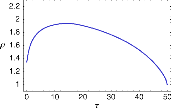
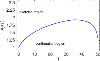
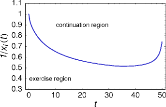
Figure 14: The function $\varrho(\tau)$ (above) and the free boundary position $x_{f}(t)=\varrho(T-t)$ (bottom-right) and the plot of the function $1/x_{f}(t)=1/\varrho(T-t)$ (bottom-left).

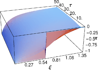
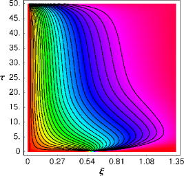
Figure 15: A 3D plot (left) and contour plot (right) of the function $\Pi(\xi,\tau)$.

In Fig. 15 we can see the behavior of the transformed function $\Pi$ in both 3D as well as contour plot perspectives. Fig. 16 depicts the initial condition $\Pi(\xi,0)$ and five time steps of the function $\xi\mapsto\Pi(\xi,\tau_{j})$ for $\tau_{j}=0.1,1,5,25,50$. A comparison of the free boundary position $x_{f}(t)=\varrho(T-t)$ as well as of its reciprocal value $1/x_{f}(t)=1/\varrho(T-t)$ obtained by our method (solid curve) and that of the projected successive over relaxation algorithm from [15] (dashed curve) is shown in Fig. 17. It is clear that our method and that of [15] give almost the same result in the one third of the time interval $[0,T]$ close to the expiration time $T=50$. On the other hand, the long time behavior when $\tau\to T$ is quite different. Notice that $\lim_{\tau\to T}\varrho(\tau)$ can be analytically computed and is equal to $1$ (see [28] or [48]). Hence the long time behavior of $\varrho$ seems to be better approximated by our method. A comparison of early exercise profiles with respect to varying dividend rate $q$ is shown in Fig. 18.

Finally, we present numerical experiments for shorter expiration times $T=0.5833$ (seven months) and $T=1$ (one year) with zero dividend rate $q=0$ and $r=0.05,\sigma=0.2$.

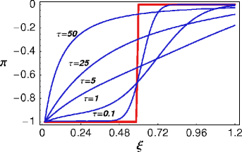
Figure 16: Profiles of the function $\Pi(\xi,\tau)$ for various times $\tau\in[0,T]$.

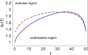
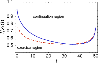
Figure 17: A comparison of the free boundary position $x_{f}(t)=\varrho(T-t)$ (left) and $1/x_{f}(t)=1/\varrho(T-t)$ (right) obtained by our method (solid curve) and that of the projected successive over relaxation algorithm from [15] (dashed curve).

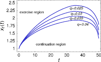
Figure 18: A comparison of the free boundary position $x_{f}(t)=\varrho(T-t)$ for various dividend yield rates $q=0.04,0.035,0.3,0.25$.

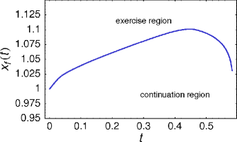
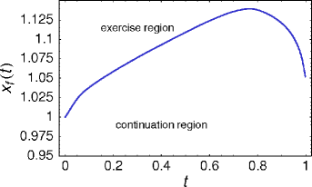
Figure 19: The free boundary position $x_{f}(t)=\varrho(T-t)$ for Asian call on assets paying no dividends ($q=0$) with expiration time $T=0.7$ (left) and $T=1$ (right).

Conclusion

In this survey paper we presented recent developments in fixed domain transformation methods applied to evaluation of the early exercise boundary for American style of options. We discussed an iterative numerical scheme for approximating of the early exercise boundary for a class of Black–Scholes equations with a volatility which may depended on the asset price as well as the second derivative of the option price. The method consisted of transformation the free boundary problem for the early exercise boundary position into a solution of a nonlinear parabolic equation and a nonlinear algebraic constraint equation. The transformed problem has been solved by means of operator splitting iterative technique. We also presented results of numerical approximation of the free boundary for several nonlinear Black–Scholes equation including, in particular, Barles and Soner model and the Risk adjusted pricing methodology model. The method of fixed domain transformation has been also applied for evaluation of early exercise boundary for American style of Asian option with arithmetically averaged strike price.

References

- [1] G. Alobaidi, R. Mallier and S. Deakin, Laplace transforms and installment options, Math. Models & Methods in Appl. Science 18(8), (2004) 1167–1189.
- [2] J. Ankudinova and M. Ehrhardt, On the numerical solution of nonlinear Black-Scholes equations, to appear in: Computers and Mathematics with Applications (2008).
- [3] J. Ankudinova and M. Ehrhardt, Fixed domain transformations and highly accurate compact schemes for Nonlinear Black-Scholes equations for American Options, in M. Ehrhardt (ed.), Nonlinear Models in Mathematical Finance: New Research Trends in Option Pricing, Nova Science Publishers, Inc., Hauppauge, to appear fall 2008.
- [4] M. Avellaneda and A. Paras, Dynamic Hedging Portfolios for Derivative Securities in the Presence of Large Transaction Costs, Applied Mathematical Finance, 1 (1994) 165–193.
- [5] M. Avellaneda, A. Levy and A. Paras, Pricing and hedging derivative securities in markets with uncertain volatilities, Applied Mathematical Finance 2 (1995) 73–88.
- [6] B. Barone-Adesi and R.E. Whaley, Efficient analytic approximations of American option values, J. Finance 42 (1987) 301–320.
- [7] F. Black and M. Scholes, The pricing of options and corporate liabilities, J. Political Economy 81 (1973) 637–654.
- [8] G. Barles and H.M. Soner, Option Pricing with transaction costs and a nonlinear Black–Scholes equation, Finance Stochast., 2 (1998) 369-397.
- [9] L.A. Bordag and A.Y. Chmakova, Explicit solutions for a nonlinear model of financial derivatives, International Journal of Theoretical and Applied finance 10 (2007) 1–21.
- [10] L.A. Bordag and R. Frey, Nonlinear option pricing models for illiquid markets: scaling properties and explicit solutions, arxiv.org/abs/0708.1568 (2007)
- [11] P. Carr, R. Jarrow and R. Myneni, Alternative characterizations of American put options, Mathematical Finance 2 (1992) 87–105
- [12] J. Chadam, Free Boundary Problems in Mathematical Finance, Progress in Industrial Mathematics at ECMI 2006, Vol 12, Springer Berlin Heidelberg, 2008.
- [13] Xinfu Chen, J. Chadam, Lishang Jiang and Weian Zheng, Convexity of the Exercise Boundary of the American Put Option on a Zero Dividend Asset, Mathematical Finance 2008 (2008) 185–197.
- [14] C.K. Cho, S. Kang, T. Kim and Y. Kwon, Parameter estimation approach to the free boundary for the pricing of an American call option, Computers and Mathematics with applications 51 (2006) 713–720.
- [15] M. Dai, Y.K. Kwok, Characterization of optimal stopping regions of American Asian and lookback options, Mathematical Finance 16 (2006) 63–82.
- [16] J.N. Dewynne, S.D. Howison, J. Rupf and P. Wilmott, Some mathematical results in the pricing of American options, Euro. J. Appl. Math. 4 (1993) 381–398.
- [17] B. During, M. Fournier and A. Jungel, High order compact finite difference schemes for a nonlinear Black–Scholes equation, Int. J. Appl. Theor. Finance 7 (2003) 767–789.
- [18] M. Ehrhardt and P. Mickens, A fast, stable and accurate numerical method for the Black-Scholes equation of American options, to appear in: International Journal of Theoretical and Applied Finance.
- [19] E. Ekström and J. Tysk, The American put is log-concave in the log-price, Journal of Mathematical Analysis and Appl. 314(2) (2006) 710–723.
- [20] E. Ekström, Convexity of the optimal stopping boundary for the American put option, Journal of Mathematical Analysis and Appl. 299(1) (2004) 147–156.
- [21] J.D. Evans, R. Kuske and J.B. Keller, American options on assets with dividends near expiry, Mathematical Finance 12 (2002) 219–237.
- [22] R. Frey and P. Patie, Risk Management for Derivatives in Illiquid Markets: A Simulation Study, Advances in Finance and Stochastics, Springer, Berlin, (2002) 137–159.
- [23] R. Frey, and A. Stremme Market Volatility and Feedback Effects from Dynamic Hedging, Mathematical Finance 4 (1997) 351–374.
- [24] R. Geske and H.E. Johnson, The American put option valued analytically, J. Finance 39 (1984) 1511–1524.
- [25] R. Geske and R. Roll, On valuing American call options with the Black–Scholes European formula, J. Finance 89 (1984) 443–455.
- [26] P. Grandits and W. Schachinger, Leland’s approach to option pricing: the evolution of a discontinuity, Mathematical Finance 11(3) (2001) 347–355.
- [27] S. Gripenberg S.O. London and O. Staffans, Volterra Integral and Functional Equations, Cambridge University Press, 1990.
- [28] A.T. Hansen and P.L. Jörgensen, Analytical Valuation of American-Style Asian Optionsl, Management Science 46 (2000) 1116–1136.
- [29] T. Hoggard, A.E. Whalley and P. Wilmott, Hedging option portfolios in the presence of transaction costs, Advances in Futures and Options Research 7 (1994) 21–35.
- [30] J. Hull, Options, Futures and Other Derivative Securities, third edition, Prentice-Hall, 1997.
- [31] H. Imai, N. Ishimura, H. Sagakuchi, Computational technique for treating the nonlinear Black-Scholes equation with the effect of transactional costs, Kybernetika 43 2007 807–816.
- [32] M. Jandačka and D. Ševčovič, On the risk adjusted pricing methodology based valuation of vanilla options and explanation of the volatility smile, Journal of Applied Mathematics 3 (2005) 235–258.
- [33] H. Johnson, An analytic approximation of the American put price, J. Finan. Quant. Anal. 18 (1983) 141–148.
- [34] C. Knessl, A note on a moving boundary problem arising in the American put option, Studies in Applied Mathematics (107) (2001) 157–183.
- [35] I. Karatzas, On the pricing American options, Appl. Math. Optim. 17 (1988) 37–60.
- [36] R.A. Kuske and J.B. Keller, Optimal exercise boundary for an American put option, Applied Mathematical Finance 5 (1998) 107–116.
- [37] M. Kratka, No Mystery Behind the Smile, Risk 9 (1998) 67–71.
- [38] Y.K Kwok, Mathematical Models of Financial Derivatives, Springer-Verlag, 1998.
- [39] H.E. Leland, Option pricing and replication with transaction costs, Journal of Finance 40 (1985) 1283–1301.
- [40] L.W. MacMillan, Analytic approximation for the American put option, Adv. in Futures Options Res. 1 (1986) 119–134.
- [41] R. Mallier, Evaluating approximations for the American put option, Journal of Applied Mathematics 2 (2002) 71–92.
- [42] R. Mallier and G. Alobaidi, The American put option close to expiry, Acta Mathematica Univ. Comenianae 73 (2004) 161–174.
- [43] G.N. Milstein, O. Reiss and J. Schoenmakers, A new Monte Carlo method for American Options, International Journal of Theoretical and Applied Finance 7 (2004) 591–614.
- [44] R. Mynemi, The pricing of the American option, Annal. Appl. Probab. 2 (1992) 1–23.
- [45] R. Roll, An analytic valuation formula for unprotected American call options on stock with known dividends, J. Finan. Economy 5 (1977) 251–258.
- [46] D. Ševčovič, Analysis of the free boundary for the pricing of an American call option, Euro. Journal on Applied Mathematics 12 (2001) 25–37.
- [47] D. Ševčovič, An iterative algorithm for evaluating approximations to the optimal exercise boundary for a nonlinear Black-Scholes equation, Canad. Appl. Math. Quarterly 15 (2007) 77–97.
- [48] D. Ševčovič, Early exercise boundary for Asian options, in preparation.
- [49] P. Schönbucher and P. Wilmott, The feedback-effect of hedging in illiquid markets, SIAM Journal of Applied Mathematics 61 (2000) 232–272.
- [50] R. Stamicar, D. Ševčovič and J. Chadam, The early exercise boundary for the American put near expiry: numerical approximation, Canad. Appl. Math. Quarterly 7 (1999) 427–444.
- [51] E.M. Stein and G. Weiss, Introduction to Fourier Analysis on Euclidean Spaces, Princeton University Press, 1971.
- [52] M. Widdicks, P.W. Duck, A.D. Andricopoulos and D.P. Newton, The Black-Scholes equation revisited: Asyptotic expansions and singular perturbations, Mathematical Finance 15 (2005) 373–391.
- [53] P. Wilmott, J. Dewynne and S.D. Howison, Option Pricing: Mathematical Models and Computation, UK: Oxford Financial Press, 1995.
- [54] Jichao Zhao, R.M. Corless and M. Davison, Compact finite difference method for American option pricing, Journal of Computational and Applied Mathematics 206 (2007) 306–321.
- [55] S.P. Zhu, A new analytical approximation formula for the optimal exercise boundary of American put options, International Journal of Theoretical and Applied Finance 9 (2006) 1141–1177.
- [56] S.P. Zhu, Calculating the early exercise boundary of American put options with an approximation formula, International Journal of Theoretical and Applied Finance 10 (2007) 1203–1227.