Wave Decay in MHD Turbulence

Abstract

We present a model for nonlinear decay of the weak wave in three-dimensional incompressible magnetohydrodynamic (MHD) turbulence. We show that the decay rate is different for parallel and perpendicular waves. We provide a general formula for arbitrarily directed waves and discuss particular limiting cases known in the literature. We test our predictions with direct numerical simulations of wave decay in three-dimensional MHD turbulence, and discuss the influence of turbulent damping on the development of linear instabilities in the interstellar medium and on other important astrophysical processes.

1. Introduction

The interstellar medium (ISM) is turbulent on scales ranging from AUs to kpc (see Armstrong et al. 1995, Elmegreen & Scalo 2004) with an embedded magnetic field that influences almost all of its properties. Turbulence is essential for understanding the ISM, the intracluster medium (ICM), the Earth’s magnetosphere, solar wind, accretion disks, etc.

The literature on astrophysical turbulence and its applications is vast (see Biskamp 2003, McKee & Ostriker 2007 and references therein). The concepts of waves and eddies are both used to describe magnetized turbulence. It is accepted that weak Alfvénic turbulence consists of waves, while for strong turbulence wave-eddy dualism is important (Goldreich & Sridhar 1995, henceforth GS95). In strong Alfvénic turbulence, nonlinear interactions damp the energy of wave-eddies over approximately one wave period. However, there are quite a few sources which exist in the turbulent environment that emit waves with different degrees of monochromaticity. These waves propagate in the turbulent medium while being modified by the medium. The evolution of such waves is of considerable astrophysical interest and has been addressed in the literature on numerous occasions. For instance, collisional and collisionless damping of fast modes in a turbulent medium was shown to differ considerably from the case when waves propagate along laminar magnetic field lines, with important consequences for cosmic ray propagation (Yan & Lazarian 2004). The latter, however, is the linear damping of waves, while the focus of this paper is the nonlinear interaction of Alfvén waves with turbulence.

Since we are addressing the subtle issue of nonlinear damping of Alfvén waves by surrounding strongly nonlinearly damped Alfvénic eddies, we feel that a discussion of the properties of MHD turbulence is due. It is well known that magnetohydrodynamics (MHD) describes the dynamics of a highly conducting fluid with magnetic field. Highly disordered quasi-stochastic flow, usually called turbulence, is generally observed in settings when the Reynolds number, the ratio of the inertial force to the viscous force, is large. When conductivity of the fluid is very low, it can be described rather well by the Navier-Stokes equations, which are, basically, the MHD equations without magnetic field. If the conductivity, however, is high, the magnetic field can no longer be ignored. In this case, the magnetic Reynolds number $Re_{m}$, or the ratio of the fluid velocity to the magnetic diffusion velocity, is large. In fact, in the turbulent flow of a conductive fluid there is a mechanism called dynamo, which increases total magnetic energy, making it more dynamically important over time (see, e.g., Vishniac et al, 2003). It is no wonder that in the astrophysical environment, where both Reynolds and magnetic Reynolds numbers are high, magnetic fields are always present and always dynamically important.

The paradoxical nature of turbulence is that even though the dissipation parameters (e.g. viscosity and magnetic diffusivity) tend to zero, the dissipation rates stay pretty much the same. The general explanation for this, as proposed by Kolmogorov (1941), is that the energy is carried from large scales through many intermediate scales down to small dissipation scales. This property is shared by turbulence in magnetized fluids. Much of the progress in understanding turbulence comes from so-called Kolmogorov models which assume a cascade of a conserved quantity, such as energy, down-scale. Once the functional dependence of the cascade decay rate, local in k-space, is known, we roughly know the spectrum of the conserved quantity (normally energy, but sometimes other quantities, such as the number of quasiparticles, enstrophy, etc.).These models do not attempt to describe all properties of turbulence, but some important ones, such as the spectrum of energy. They essentially assume self-similarity, so they don’t describe deviations from self-similarity, known as intermittency. The level of sophistication of these so-called mean field models is enough for many applications.

While the spectrum of hydrodynamic incompressible turbulence is well-established, strong MHD turbulence is an area of active research (e.g. Montgomery & Turner (1981), Shebalin, Matthaeus & Montgomery (1983), Higdon (1984)). Numerical research (Cho & Vishniac 2000, Maron & Goldreich 2001, Cho, Lazarian & Vishniac 2002, Cho & Lazarian, 2002, 2003, Müller, Biskamp & Grappin 2003) is roughly consistent with a particular model of strong turbulence, called Goldreich-Sridhar model (Goldreich & Sridhar, 1995). This mean-field model predicts structural anisotropy with respect to the magnetic field according to so-called critical balance, $k_{\perp}\delta v\sim k_{\|}v_{A}$, as well as a $k^{-5/3}$ energy spectrum.

The wave dissipation rate has two major applications. First, if it is directly measured, either in experiment, observation, or numerical simulation, it can be used as a test of turbulence itself, and, in certain mean-field models of turbulence, since the latter rely on the phenomenologically estimated value of the mean dissipation rate for every particular scale.

The other application is turbulent damping of linear instabilities. If the instability growth rate is smaller than the turbulent damping rate, the instability does not develop. This can have numerous consequences. For instance, it has been customary to compare the instability rate to the viscous or magnetic dissipation rates. Because of this, almost any “large scale” perturbation with positive imaginary part of the frequency obtained from linear analysis has been thought to develop a growing unstable mode. It is possible, however, that this instability is slow enough to be damped by the turbulent field. This way the unstable configuration is stabilized, provided it is not disrupted by turbulence itself. In the case when turbulence itself is generated by an instability, the turbulent dissipation rate will provide a powerful generic mechanism for nonlinear saturation of the instability. Such a generic saturation mechanism is highly desirable, since typically nonlinear saturation models are very specific to the instability in question and contain quite a number of assumptions.

One example of the application of turbulent damping rates to astrophysics is the study of the escape of high energy Cosmic Rays (CRs) from our Galaxy (Yan & Lazarian 2002, 2004, Farmer & Goldreich, 2004). Lazarian and Beresnyak (2006) developed a model in which the low-energy CR mean free path is effectively reduced in the presence of compressive motions due to the CR-Alfvén anisotropic instability.

Previous works that considered the turbulent wave dissipation include Hollweg (1984), Similon & Sudan (1989), Kleva & Drake (1992), Farmer & Goldreich (2004), Bian & Tsiklauri (2007) and others.

In our paper we develop a model of turbulent dissipation which is purely nonlinear (does not depend on either $Re$ or $Re_{m}$) and has self-similar power-law dependencies on the wavenumber, which is characteristic of turbulence. We also explain why parallel waves (with wavevector parallel to the field) decay in a different way than perpendicular waves. We give a general formula for the decay rate for arbitrarily directed waves. The study of the turbulent decay of parallel directed waves by Farmer & Goldreich (2004) was motivated by the fact that such waves have the highest instability grows rate for CR-plasma instabilities such as the streaming and the anisotropy instabilities (e.g., Kulsrud 2005).

In what follows we describe the model of turbulent dissipation and derive the formula for the dissipation rate in §2, provide numerical evidence for turbulent wave dissipation in §3, discuss astrophysical implications in §4, mention competing mechanisms for wave damping in §5, discuss previous work in §6 and summarize our results in §7.

2. Wave dissipation

The equations of incompressible ideal MHD,

$$\partial_{t}{\bf w^{+}}+({\bf w^{-}}\cdot\nabla){\bf w^{+}}=-\nabla P,$$ (1)

$$\partial_{t}{\bf w^{-}}+({\bf w^{+}}\cdot\nabla){\bf w^{-}}=-\nabla P,$$ (2)

$$\nabla\cdot{\bf w^{+}}=\nabla\cdot{\bf w^{-}}=0,$$ (3)

written in terms of Elsasser variables ${\bf w^{+}=v+b}$ and ${\bf w^{-}=v-b}$, where ${\bf v}$ is the velocity and ${\bf b}$ is the magnetic field in velocity units ${\bf b=B}/(4\pi\rho)^{1/2}$, bear close resemblance to the Navier-Stokes equations. This resemblance is somewhat superficial, since ${\bf w^{+}}$ and ${\bf w^{-}}$ do not transform the same way velocity transforms under Galilean transformations. Due to this fact, there is usually some residual, or local mean magnetic field, that cannot be excluded by the choice of frame of reference (Kraichnan, 1965). If we go to sufficiently small scales the decaying perturbation fields will be much smaller than the local mean field. This case is called sub-Alfvénic turbulence. The important conservation laws in non-dissipative MHD is the conservation of the integrals $\int|w^{+}|^{2}d^{3}x$ and $\int|w^{-}|^{2}d^{3}x$, which are the analogs of conservation of energy in the Navier-Stokes equations. This allows us to build phenomenology of energy transfer in the spirit of Kolmogorov (1941) for each of the ${\bf w^{+}}$ and ${\bf w^{-}}$ variables with two different dissipation rates. The setup when those dissipation rates are equal is called balanced turbulence, while the opposite case is called imbalanced or cross-helical turbulence.

The major difference between the incompressible Navier-Stokes and MHD equations is that the characteristics of the latter, due to the presence of local magnetic field, are always wave-like, with the speed of the perturbation being $v_{A}$. While it is not possible to have waves in incompressible hydrodynamics, it is possible to have waves or wave-like perturbations in incompressible MHD. According to the GS95 model, most perturbations produced by turbulence cannot be called well-defined waves. But there are other perturbations generated, for example, by instabilities, which, as we will demonstrate in this paper, have frequency much larger than decay rate and, therefore, can be called waves.

This paper is focused on the study of the decay of a small perturbation in stationary forced turbulence. Unlike decaying turbulence, where the energy decays self-similarly, or as a power-law with time, the decay of a small perturbation in stationary turbulence will be exponential. This statement is based on the general concept of the flow of energy through scales, which underlies all Kolmogorov-type models. Indeed, in Kolmogorov models, the decay rate is some function of the perturbation strength and the length scale: $\gamma_{\rm turb}(\delta v,\lambda)$. For example, in strong hydrodynamical turbulence, $\gamma_{\rm turb}=\delta v/\lambda$. Since the wave amplitude is small, it can not significantly affect $\delta v$. Therefore the dissipation rate will be constant, meaning that the wave will decay exponentially.

In this paper we only consider the Alfvén and pseudo-Alfvén waves that exist in incompressible turbulence. The study of the decay of all three wave modes in generic compressible turbulence is a task that will be addressed elsewhere.

Now we will provide a phenomenological description of wave decay and the formula for the decay rate for arbitrarily directed waves. To highlight the general problem we first consider parallel waves. According to the second-order perturbation theory, such waves are not cascaded (e.g., Galtier et al 2002). Does this property necessarily apply to strong turbulence? Farmer & Goldreich (2004) argued that this is not the case, addressing the issue of the wave propagation parallel to the local magnetic field when the effective perpendicular wavenumber is obtained by so-called field wandering. Let us imagine a plane wave with very large perpendicular correlation length, corresponding to $k_{\perp}=0$ and finite parallel correlation length $\Lambda$, corresponding to $k_{\|}=1/\Lambda$. This wave, moving a distance of $\Lambda$, will get disrupted by field wandering, as various pieces of this wave propagate along its local field direction, which is slightly different along the transverse spread of the wave. Note that only field-wandering from the counter-propagating waves will contribute to this process, as the co-propagating waves will move exactly the same distance, being stationary in the frame of the wave. The “effective” perpendicular wavenumber $k_{\perp,{\rm eff}}$ is determined by the condition $k_{\perp,{\rm eff}}=(\delta B/B)k_{\|}$, where we use $\delta B$ of counter-wave on scale $1/k_{\perp,{\rm eff}}$.

The arguments above can be generalized for the case of an arbitrarily directed wave in the following way. While the wave is being decorrelated by turbulence, it obtains a new “effective” $k_{\perp,{\rm eff}}$ from the vector sum of the original $k_{\perp}$ and the one produced by turbulent field wandering. The effective $k_{\perp,{\rm eff}}$ in the RMS sense will be the square mean of the two. If the original wave has a pitch angle $\theta$ with respect to the field and a wavenumber magnitude of $k$, its effective perpendicular wavenumber will be determined by the equation

$$k_{\perp,{\rm eff}}=k(\sin^{2}\theta+(\delta B/B)^{2}\cos^{2}\theta)^{1/2},$$ (4)

or, if we assume the GS95 scaling $\delta B/B\sim k_{\perp}^{-1/3}$,

$$k_{\perp,{\rm eff}}=k(\sin^{2}\theta+(k_{\perp,{\rm eff}}L)^{-2/3}\cos^{2}\theta)^{1/2}.$$ (5)

According to the arguments above, we should include only the part of $\delta B/B$ which corresponds to the counter-wave, since co-propagating perturbations do not influence the structure of the wave. This is due to the exact solution of the incompressible MHD which involves only one wave species of arbitrary amplitude. In eq. (5), for the sake of simplicity, we omitted the coefficient $1/2$ before $\delta B/B$ which would indicate that only half of the perturbations contribute to the decorrelation effect.

It is easy to verify from eq. (5), that for perpendicular modes $k_{\perp,{\rm eff}}=k\sin\theta=k$ (as if field wandering is unimportant), while for parallel modes, $k_{\perp,{\rm eff}}\sim k^{3/4}$ (as in Farmer & Goldreich 2004).

The decay rate is determined by the $k_{\perp,{\rm eff}}$ we calculated from (5):

$$\gamma=v_{A}k_{\perp,{\rm eff}}^{2/3}L^{-1/3}.$$ (6)

Eq. (6) deserves a more detailed explanation. While cascading of perturbations in weak turbulence have resonant character, that is, they require counter-waves with equal and oppositely directed ${\bf k_{\|}}$ (e.g., Ng & Bhattachargee 1996, Goldreich & Sridhar 1997, Galtier et al 2002), strong turbulence involves nonlinear perturbations where strict resonance condition is not required. This can be demonstrated if we consider a cascaded perturbation as a passively advected vector field. This approach is valid as long as the amplitude of this sample or test perturbation is small enough to avoid any back-reaction to fully developed, balanced strong turbulence. Now, according to critical balance of GS95, the transverse structure of this passively advected field is strongly perturbed by counter-waves with the same $k_{\perp}$ after traveling a distance of $1/k_{\|}=k_{\perp}^{-2/3}L^{1/3}$. On the other hand, according to GS95, this is the correlation length of the counter wavepacket, so the “next” perturbation will be applied to our test field incoherently. Therefore, these perturbations of the transverse structure of the test field are irreversible and can be called cascading in perpendicular direction. Our main point here is that the lateral structure of the test field is irrelevant for its cascading (unless the lateral structure produces the transverse structure by field wandering), as long as cascading happens in strong GS95 turbulence.

The formulae (5) and (6) give the general dependence of the decay rate $\gamma$ on arbitrarily directed (oblique) waves with wavevector $k$ and pitch-angle $\theta$. This dependence is, in general, not a power-law of $k$. There are two limiting cases of the perpendicular directed and the parallel directed waves which give power-laws, namely

$$\gamma_{\perp}=v_{A}k^{2/3}L^{-1/3},\ \ \ \gamma_{\|}=v_{A}k^{1/2}L^{-1/2}.$$ (7)

Fig. 1 shows the dependence of the decay rate $\gamma$ on the wavevector $k$ for a variety of pitch angles $\theta$ with respect to the magnetic field.

Figure 1.— The relative decay rate versus wavenumber for different angles as obtained from Eqs. 5 and 6.

3. Numerical Results

We have conducted a series of 71 incompressible three-dimensional $320^{3}$ MHD simulations with stochastic turbulent driving. We used a pseudo-spectral code to solve Eqs. 1-3 and introduced linear dissipation as an energy sink. We used relatively low-order (6th order) hyperdiffusion to extend the inertial range while avoiding a strong bottleneck effect. The turbulent driving supplied energy between $k=2$ and $3.5$ while most of the dissipation happened around $k=70$. We regarded the interval $k=5$ to $50$ as an inertial interval of turbulence. Simulations had an external magnetic field and the driving was tuned to produce strong turbulence which was nearly isotropic around the driving scale. More details of the code and the driving can be found in Cho and Vishniac (2000).

In this series one of the simulations was without wave driving, and all others were driven with a plane wave with a particular wave vector ${\bf k}$. The turbulent driving and the initial conditions in all series were exactly the same. The initial conditions were taken from another turbulent simulation with driving that ran for around 20 Alfvén times. We waited for about 0.3 Alfvén times for the wave to reach saturation. We chose the wave driving amplitude so that the saturated wave does not incur any significant back-reaction to turbulence. After this the wave driving was switched off but the turbulent driving continued just like in the simulation without wave driving.

As expected, after the wave reached saturation, it was no longer plane-parallel and its energy distribution in k-space was affected by both field line wandering and strong turbulent cascading. It is more appropriate to say that the simulation box was filled with a collection of wave packets which had the dispersion in the direction of ${\bf k}$ and the dispersion in $k_{\|}$ and $k_{\perp}$ that comes from turbulent decorrelation and the corresponding uncertainty relation. In Fig. 2 we presented a visual representation of the distribution of wave energy that was initially driven as the parallel wave with $k_{\|}=17$ (in cube size units) and reached saturation.

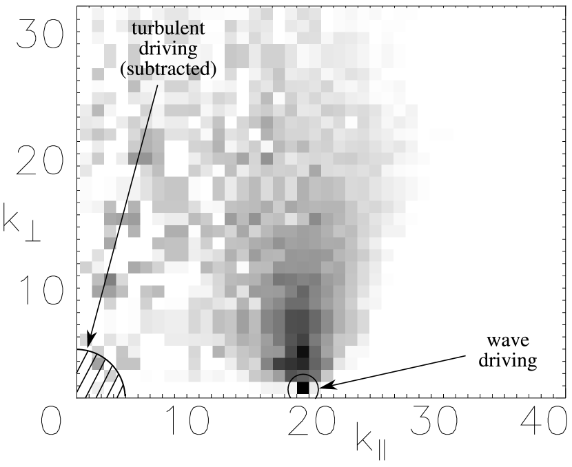
Figure 2.— Decorrelation of the parallel-propagating wave by turbulent field wandering. Darker areas indicate larger wave energy. The wave is decorrelated and cascaded primarily in the direction perpendicular to the magnetic field.

The wave energy was obtained by subtracting the results of the simulation with and without wave driving. We summed the result of subtraction only over the relevant regions in $k$-space, to reduce errors. We note again, that driving, although being turbulent-like, was predetermined, and within our short simulation times (about 0.6 Alfvén times) chaos in motions on large scales was not yet able to develop. This was confirmed by the fact that the result of subtraction was mostly positive and significantly differed from zero only around the region where we pumped the wave. One notable exception from this rule was the velocity at k=0, or the mean velocity. It increased, which is interpreted as a transfer of momentum from the wave to the fluid. We have carried out a total of 70 $320^{3}$ simulations with different values of the wave ${\bf k}$ vector which have covered the inertial range of our turbulent simulation from $k=10$ to $k=40$ with different angles with respect to the mean magnetic field.

After the wave driving was switched off, the energy of the wave started to decay exponentially (see Fig. 3). We measured the decay rate by fitting a decay curve. Fig. 4 shows the dependence of the decay rates on the $k$ value and on the angle of original inclination of wave to the magnetic field (the angle $\theta$ between ${\bf k}$ and ${\bf B}$). As we see, for waves parallel to the external field the decay rate follows a $k^{1/2}$ law (see also Farmer & Goldreich 2004). The theoretical curves for the different inclinations that were fitted into numerical values of $\gamma$, unexpectedly, have slightly different values for the outer scale $L$. We believe that this could be either due to the fact that the wavelengths that we considered were relatively close to the driving scale, or the fact that we simulated trans-Alfvénic turbulence.

Figure 3.— The evolution of the oblique wave energy during the driving and decay stages. The wave driving was at $(k_{\|},k_{\perp})=(12,12)$ in code units, approximately $(4,4)L^{-1}$.

Figure 4.— The dependence of the decay rate on the magnitude of the wavevector for different angles between ${\bf k}$ and ${\bf B_{0}}$ in a direct 3D numerical simulation (points), fitted with curves obtained from eqs. 5 and 6 (lines).

4. Applications of Turbulent Damping

The damping of Alfven waves with ${\bf k}$ parallel to the magnetic field was invoked by Farmer & Goldreich (2004) in the context of the damping of the streaming instability by ambient turbulence (first mentioned in Yan & Lazarian 2002). They estimated that with the modest level of turbulence in our Galaxy, the streaming instability will be suppressed for cosmic rays with energies higher than about 100 GeV; therefore such cosmic rays can freely propagate along the magnetic field lines. Lazarian & Beresnyak (2006) have used turbulent damping as one of the mechanisms that limits the CR anisotropy instability which occurs in a magnetized fluid in the presence of compressible turbulence. This instability greatly decreases the CR’s mean free path. However, due to turbulent damping, there is a high energy limit of around 1000 GeV (for our Galaxy) for this mechanism. Particles with energy higher than this limit will be unaffected by the instability and scattered primarily through other mechanisms, such as direct interaction with MHD modes (Chandran 2000, Yan & Lazarian 2002, 2004, 2007).

The influence of the turbulent decay to the development of instabilities can lead to the various interesting astrophysical effects. Let us consider one example. In a recent paper, Everett et al (2007) (henceforth E07) considered a model of launching the Galactic wind by CR pressure (see also Breitschwerdt et al, 1991). They argued that CR pressure is necessary to launch the wind, since thermal pressure is too small. One of the critical assumptions of this model is that the streaming instability operates effectively and allows CRs to exchange momentum with the plasma. Let us now assume that the streaming instability is damped by turbulence. According to Farmer & Goldreich (2004), if the amplitude of turbulence is similar to that of our Galaxy, the damping of the streaming instability will affect CRs with energies higher than 100 GeV, making them effectively disconnected from the background plasma and able to escape. If most of the energy (and the momentum) of CRs are in the lowest energy CRs, as E07 originally assumed, this would present no problem for their model. It is believed, that our Galaxy, on average, has a relatively steep spectrum of CRs, between the slopes of $-2.6$ and $-3.1$, justifying this assumption. However, the winds are most likely to be launched from the sites of intensive CR production, such as regions with many supernova shocks. Some modern theories of shock acceleration with precursor favor a rather shallow spectrum of the accelerated particles, such as shallower than $-2$ (Malkov & Drury 2001) . CRs with such a spectrum have most of their energy and momentum in higher energy particles that can freely escape because of damping of the streaming instability and, therefore, CR pressure is too weak to launch the wind. The existence of the Galactic wind would therefore suggest that it is always being launched by a CR population with a steep spectrum, or that these winds have very low level of turbulence. Since we cannot directly observe the spectrum of the CRs near acceleration sites such information about the slope being shallower or steeper than $-2$ can be used to limit theories of CR acceleration in shocks.

The other application of energy dissipation of Alfvén waves is the problem of coronal heating. It has been long known that due to the very small values of viscous and magnetic dissipation coefficients, ohmic and viscous heating are unlikely to dissipate Alfvén waves significantly. On the other hand, we know that a relatively small fraction of energy of waves actually escapes the coronal region. Turbulent dissipation can deal with this problem, since it provides much higher dissipation rates than ohmic and viscous heating, and, unlike the latter, does not depend on the Reynolds numbers $Re$ and $Re_{m}$. Parker (1991) noted, however, that in the corona, the stochastic component of the field mostly consists of waves propagating in one direction, outwards from the Sun. In our terminology this is a strongly imbalanced case. While there is certainly a strong imbalance close to the photosphere near the source of the waves, the situation in the upper solar corona could be closer to balanced turbulence due to various mechanisms that allow waves to reflect back, such as the geometry of the guiding magnetic field, the parametric instability, etc. Despite coronal heating still being a poorly understood process there are few things that we would like to note with regards to our model. First of all, our model does not consider dissipation in imbalanced turbulence, due to the fact that models of strong imbalanced turbulence are being developed (see Beresnyak & Lazarian 2007 and references therein, see Discussion). Secondly, we only considered waves with small amplitudes that do not produce strong back-reaction to turbulence. We hope, however, that the present work can provide insight into a more complicated picture that will include imbalanced turbulence, reflection of waves, etc.

There is also the problem of launching winds, such as a stellar wind, by momentum from waves. It is similar to the previous problem, in that we need mechanisms of wave reflection, in order to generate turbulence, otherwise waves will freely escape. It is well known that the solar wind is strongly imbalanced close to the Sun, but becomes less imbalanced at larger distances, almost reaching equipartition between waves near the Earth’s orbit. Roberts et al (1987) suggested that this was due to the dominance of the kinetic energy on the outer scale.

5. Competing Mechanisms of Damping

While the ohmic and viscous dissipation rates decrease very rapidly with increasing wavelength, as $k^{2}$, there are a number of mechanisms of Alfvén wave dissipation that, in principle, can compete with turbulent dissipation. The dissipation mechanisms can be subdivided into linear and nonlinear mechanisms. We call it a linear mechanism when the decay rate does not depend on the amplitude of the wave. Such mechanisms include viscous damping, turbulent damping (even though the turbulence itself is a nonlinear process), collisionless (Landau) damping, and the resonance damping. Nonlinear damping mechanisms have a decay rate that depends on the wave amplitude. These include nonlinear Landau damping, wave steepening, etc.

Nonlinear Landau damping (e.g., Kulsrud 2005) requires two waves with close frequencies and a population of ions that is in resonance with the beat wave of those two waves. While, generically, the decrement of this damping is proportional to the frequency, it has a nonlinear $(\delta B/B_{0})^{2}$ factor that limits damping to high amplitude waves. Note that the turbulent damping mechanism that we consider in this paper has a substantial limitation in that the wave amplitude has to be small enough to not back-react on the turbulence itself. Thus, nonlinear damping mechanisms and the linear (with respect to the wave amplitude) turbulent damping are, in a sense, complimentary to each other (see fig. 5). Another nonlinear mechanism of damping is wave steepening (e.g., Cohen & Kulsrud, 1974). This mechanism is also supposed to have $\gamma\sim kv_{A}(\delta B/B_{0})^{2}$.

Figure 5.— Dominating dissipation mechanisms for various wave lengths and wave amplitudes in the ICM or hot ISM. Linear collisionless (Landau) damping acts only on the pseudo-Alfven mode, while nonlinear Landau damping and turbulent damping operate on both modes.

The prominent linear mechanism of damping is so-called resonance damping (e.g., Hollweg, 1984). Unlike previously mentioned mechanisms that are considered in a homogeneous medium and usually work equally well in any geometry, this linear damping mechanism appears when, due to the specific boundary conditions or inhomegeneity of the flow, the so-called Alfvenic resonance appears. This resonance corresponds to the flow speed being equal to the phase speed of the Alfvenic wave. The resonance is typically the $1/x$ type divergence for the magnetic field and velocity. Notably, the dissipation provided by this resonance does not depend on viscosity or magnetic diffusivity (Kappraff & Tataronis 1977). The dissipation rate can be calculated from the ideal MHD equations with $\nu=\eta=0$ using contour integrals (e.g., Livshitz & Pitaevskii 1981, Pariev & Istomin 1996). The Alfven resonance of the flow has been proposed as a prominent candidate for an in-situ acceleration mechanism in jets (Beresnyak, Istomin & Pariev 2003). Resonance damping usually provides damping rates that are a fraction of the wave frequency. It is considered to be important when the wave length is of order the scale at which boundary conditions are set. In jets we expect turbulent damping to be more important than resonance damping (if the latter is present) for wavelengths that are much smaller than the jet’s diameter, assuming that for these wavelengths the medium can be treated as homogeneous.

6. Discussion

This paper deals with wave dissipation in a balanced MHD turbulence. The more general imbalanced case was not considered for a variety of reasons. First, the theory of strong imbalanced MHD turbulence is still being developed (Lithwick, Goldreich & Sridhar 2007, Beresnyak & Lazarian 2007). On the other hand, if we adopt the model of imbalanced turbulence presented in Beresnyak & Lazarian 2007 (furthermore BL07) a number of questions arise. Most importantly, we will be unable to reproduce the statement of §2 that the cascading of the wave is irrelevant to its lateral structure. This is due to the fact that neither the strong nor the weak wave from BL07 has a critical balance with itself (i.e. $k_{\|}v_{A}=k_{\perp}\delta v$ does not hold if all quantities refer to the same wave, instead BL07 provides a different expression for the critical balance of each wave). Therefore there is no guarantee that we can use the strong cascading formula, at least when the wave has a large $k_{\|}$.

An attempt to include irregularities of magnetic field lines due to turbulence to increase predicted dissipation in solar corona was made in Silimon & Sudan (1989). Their model relies on a description of turbulent magnetic field lines as divergent with a specific Lyapunov constant, or exponentiation rate $\lambda$. We argue that this is not a proper description of turbulent fields in developed turbulence because such fields are approximately self-similar and do not have any designated scale in its inertial interval. In developed turbulence every scale has its own exponentiation rate. Silimon & Sudan (1989) give a formula for dissipation length which is inversely proportional to the Lyapunov constant (which is not specified, but estimated) and only weakly (logarithmically) proportional to the wavenumber. It also depends on magnetic Reynolds number. This paper, in contrast, advocates purely nonlinear dissipation rates that do not depend on $Re_{m}$ or $Re$. Parker (1991) criticized Silimon & Sudan’s approach of using stochastic field lines to increase dissipation by noting that the stochastic component of the field is itself part of the waves propagating outwards along the field. We commented on this controversy previously by noting that one has to have a mechanism to reflect the waves back, otherwise they escape freely.

Kleva & Drake (1992) have studied nonlinear dissipation of waves in the presence of a stochastic field on an outer scale by numerical methods. They confirmed that the dissipation of large scale waves does not depend on dissipation coefficients, while for small scale waves it approached the viscous and resistive limit. However, their stochastic field was not turbulent, but rather a predetermined field on the outer scale. Also, the damping rate they measured did not depend on wavevector as a power-law.

Bian & Tsiklauri (2007) have considered mixing of Alfvén wavepackets in chaotic magnetic fields. They obtained an analytical expression for the advection-diffusion of wavepackets using a WKB approximation and claimed that the stationary wave energy spectrum is $k^{-1}$. We feel that the WKB method is not the appropriate tool to derive turbulent dissipation, as it requires that the wave should have wavelengths that are much smaller than the underlying perturbations, while in turbulence the most effective nonlinear dissipation comes from scales comparable with the wavelength.

Hollweg (1984) considered dissipation of Alfvén waves in coronal loops, primarily due to resonance mechanism, but also speculated on turbulent heating. He took the Kolmogorov dissipation rate (which is a decay that happens on a kinetic timescale $\lambda/v$) with the perturbation length scale as wavelength and the RMS wave velocity as perturbation velocity. This way he obtained dissipation which is compatible with heating in coronal loops as well as coronal holes. We have to note, however, that propagating waves do not necessarily generate turbulence and even if there is a flux of waves in both directions, there are certain requirements for MHD turbulence to be strong turbulence and have the Kolmogorov dissipation rate. For example, in the context of coronal loops, with a strong guide field, it is easy to imagine a situation where turbulence is not strong on the outer scale, therefore it has dissipation rate lower than Kolmogorov.

7. Summary

In this paper we demonstrated the following:

1. Parallel and perpendicular directed waves are dissipated in different ways. Perpendicular waves are cascaded naturally by counter-waves, while parallel waves are first decorrelated by the field wandering and then cascaded.

2. In the inertial interval of sub-Alfvénic turbulence, parallel waves are damped more slowly than perpendicular waves with the same wavenumber. The decay rate for the parallel wave is much smaller than its frequency, it is not eddy but a well-defined wave.

3. In a homogeneous medium with open boundaries turbulent dissipation is more effective than the other dissipation mechanisms, provided that the wave amplitude is sufficiently small and the wavelength is in the inertial interval of turbulence.

References

- (1) Beresnyak, A. R., Istomin, Ya. N., Pariev, V. I. 2003 A&A, 403, 793
- (2) Beresnyak, A., Lazarian, A. 2006, ApJ, 640, L175
- (3) Beresnyak, A., Lazarian, A. 2007, astro-ph/0709.0554
- (4) Bian, N., Tsiklauri, D. 2007, astro-ph/0709.0260
- (5) Boldyrev, S. 2005, ApJ, 626, L37
- (6) Boldyrev, S. 2006, Phys. Rev. Lett., 96, 115002
- (7) Breitschwerdt, D., McKenzie, J. F., & Völk, H. J. 1991, A&A, 245, 79
- (8) Chandran B., 2000, Phys. Rev. Lett., 85, 4656
- (9) Cho, J., & Lazarian, A. 2002, Phys. Rev. Lett. 88, 24, 245001
- (10) Cho, J., & Lazarian, A. 2003, MNRAS, 345, 325
- (11) Cho, J., Lazarian, A., & Vishniac 2002, ApJ, 564, 291
- (12) Cho, J. & Vishniac, E. 2000, ApJ, 539, 273
- (13) Cohen, R. H., Kulsrud, R. M. 1974 Phys. Fluids, 17, 2215
- (14) Everett, J.E., Zweibel E.G., Benjamin, R.A., McCammon, D., Rocks, L., Gallagher, J. S. III 2006, ApJ, in press
- (15) Farmer, A.J., & Goldreich, P., 2004, ApJ, 604, 671
- (16) Galtier, S., Pouquet, A., Mangeney, A. 2005, Phys. Plasmas, 12, 092310
- (17) Galtier, S., Nazarenko, S.V., Newell, A.C., & Pouquet, A. 2002, ApJ, 564, L49
- (18) Gogoberidze, G. 2007, Phys. Plasmas, 14, 022304
- (19) Goldreich, P., & Sridhar, S., 1995, ApJ, 438, 763
- (20) Goldreich, P., & Sridhar, S., 1997, ApJ, 485, 680
- (21) Grappin, R., Pouquet, A., & Léorat, J. 1983 A&A, 126, 51
- (22) Higdon J. C., 1984, ApJ, 285, 109
- (23) Hollweg, J. 1984, ApJ, 277, 392
- (24) Kappraff, J. M., & Tataronis, J. A. 1977, J. Plasma Phys., 18, 209
- (25) Kleva, R. G. & Drake, J. F. 1992, ApJ, 395, 697
- (26) Kolmogorov, A. 1941, Dokl. Akad. Nauk SSSR, 31, 538
- (27) Kraichnan, R.H., Phys. Fluids 8, 1385 (1965)
- (28) Kulsrud R., 2004, Plasma Physics for Astrophysics, Princeton, NJ, Princeton University Press
- (29) Lazarian, A., Beresnyak, A. 2006, MNRAS, 373, 1195
- (30) Lifshitz, E. M. & Pitaevskii, L. P. 1981, Physical kinetics, New York: Pergamon Press
- (31) Lithwick, Y., Goldreich, P., & Sridhar, S. 2007, ApJ, 655, 269
- (32) Malkov, M. A., Drury, L.O’C. 2001, Rep. Prog. Phys, 64, 429
- (33) Maron, J., & Goldreich, P. 2001, ApJ, 554, 1175
- (34) McKee, C. F. Ostriker, E. C. 2007 Ann. Rev. of Astron. & Astrophys., 45, 565
- (35) Montgomery, D.C., & Turner, L. 1981, Phys. Fluids, 24, 825
- (36) Müller W.-C., Biskamp, D., & Grappin, R 2003, Phys. Rev. E, 67, 066302
- (37) Ng, C.S., Bhattacharjee, A. 1996, ApJ, 465, 845
- (38) Pariev V. I., Istomin Ya. N., 1996, MNRAS, 281, 1
- (39) Parker, E. N. 1991, ApJ, 372, 719
- (40) Roberts, D. A., Goldstein, M. L., Klein, L. W., Matthaeus, W. H. 1987, J. of Geophys. Res., 92, 12023
- (41) Shebalin, J.V., Matthaeus, W.H., & Montgomery, D. 1983, J. of Plasma Phys., 29, 525
- (42) Schekochihin, A. A., Maron, J. L., Cowley, S. C., McWilliams, J. C. 2002, ApJ, 576, 806
- (43) Similon, P., & Sudan, R. 1989, ApJ, 336, 442-453
- (44) Vishniac, E. T., Lazarian, A., & Cho, J. 2003, in Turbulence and Magnetic Fields in Astrophysics Ed. by E. Falgarone, T. Passot., Lecture Notes in Physics, 614, 376
- (45) Yan H., Lazarian A., 2002, Phys. Rev. Lett., 89, 281102
- (46) Yan H., Lazarian A., 2004, ApJ, 614, 757
- (47) Yan H., Lazarian A., 2007, astro-ph/0710.2617