Magnetoasymmetric current fluctuations of single-electron tunneling

Abstract

We determine the shot noise asymmetry of a quantum dot under reversal of an external magnetic field. The dot is coupled to edge states which invert their chirality when the field is reversed, leading to a magnetoasymmetric electrochemical potential in the nanostructure. Surprisingly, we find an exact relation between the magnetoasymmetries corresponding to the nonlinear conductance and the shot noise to leading order in the applied bias, implying a higher-order fluctuation-dissipation relationship. Our calculations also show a magnetoasymmetry of the full probability distribution of the transferred charge.

I Introduction

Recently, it has been theoretically demonstrated san04 ; spi04 ; but05 ; pol06 ; mart06 ; and06 and experimentally verified rik05 ; wei06 ; mar06 ; let06 ; zum06 ; ang07 ; har08 that the Onsager-Casimir reciprocity relations ons ; cas cannot be, in general, extended to mesoscopic transport far from equilibrium. Departures of microreversibility at equilibrium have been related to the interaction of the nanostructure with an environment driven out of equilibrium.san08 In both cases, it is found that the current flowing through the system is not invariant under reversal of the external magnetic field, leading to the observation of magnetoasymmetries solely due to the asymmetric properties of the internal electrostatic potential. Thus, the effect is induced purely by electron interactions.

Previous literature has discussed the size of the magnetoasymmetries for the electric conductance. Here, we are concerned with the shot noise, which is known to offer a complementary and, quite often, unique tool to probe electronic transport in quantum correlated nanostructures.bla00 Shot noise has been shown to reveal electronic entanglement detection in mesoscopic interferometers,los00 dynamical spin blockade in dots attached to ferromagnetic leads,cot04 quantum shuttling in nanoelectromechanical systems,nov04 nonequilibrium lifetime broadenings in cotunneling currents,uts06 and quantum coherent coupling in double quantum dots,kie07 just to mention a few.

It is worth noting that the linear conductance and the equilibrium noise are related each other via the linear fluctuation-dissipation theorem, which is a general statement about the response of a system near equilibrium and its dynamical fluctuations induced by random forces.mar08 For mesoscopic conductors the theorem is expressed as the Johnson-Nyquist formula between equilibrium current fluctuations and the linear conductance.bla00 Both the linear conductance and the current fluctuations at equilibrium obey reciprocity relations.but86 At nonequilibrium, however, Onsager’s microreversibility is generally not fulfilled. Notably, our calculations explicitly show an exact relation between both magnetoasymmetries corresponding to the noise susceptibility and the nonlinear conductance to leading order in the applied voltage bias, implying a higher-order fluctuation-dissipation relationship. Recent works foe08 ; sai08 find similar fluctuation relations.

II The system

We show our result considering a simple but paradigmatic mesoscopic system—a quantum dot in the Coulomb blockade regime for which the charge is quantized and transport is blocked at low temperature unless charging energy is supplied by external voltage.kou97 ; bee91 We study a dot coupled to two chiral states for94 ; kir94 (filling factor $\nu=1$) propagating along the opposite edges of a quantum Hall conductor, as shown in Fig. 1. For positive magnetic fields $B>0$ carriers in the upper (lower) edge state move from the left (right) terminal to the right (left) terminal. The current flow is reversed for $B<0$. Coupling between the dot and the edge states takes place via tunnel couplings $\hbar\gamma_{1}$ and $\hbar\gamma_{2}$ and capacitive couplings $C_{1}$ and $C_{2}$.

We consider a single energy level $E_{0}$ which can be externally tuned with a gate voltage. ($E_{0}$ is a kinetic energy invariant under $B$ reversal). The dot lies deep in the Coulomb-blockade regime for which $E_{0}+e^{2}/C$ (with $C=C_{1}+C_{2}$) is well above the electrochemical potentials $\mu_{\alpha}=E_{F}+eV_{\alpha}$ ($\alpha=L,R$) of both left ($L$) and right ($R$) leads, $E_{F}$ being the common Fermi energy. We assume that each edge state is in equilibrium with its corresponding injecting reservoir. Therefore, they act effectively as massive electrodes with well defined electrochemical potentials. Without loss of generality, we take $V_{L}=-V_{R}=V/2$ with $V$ the applied bias voltage.

For temperatures $k_{B}T$ and voltages low enough, $k_{B}T,eV\ll e^{2}/C$ (but $k_{B}T$ sufficiently high to neglect Kondo correlations), the charging energy $e^{2}/C$ is the dominant energy scale of the problem and double occupation in the dot is negligible. In the master equation approach, the charging state of the dot is given by an integer number of electrons, $n$. We assume that quantum coherence between states with differing $n$ is lost, as occurs in the pure Coulomb blockade regime. For definiteness, we consider spin polarized carriers, although the model can be easily extended to the spinful case. Thus, the dot can be either in the empty state ($n=0$) or in the occupied state ($n=1$) with instantaneous occupation probability $p_{n}(t)$ at time $t$. The main transport mechanism is via single-electron tunneling ($\gamma_{1},\gamma_{2}\ll k_{B}T/\hbar$) and we can write quantum rate equations for $p_{0}(t)$ and $p_{1}(t)$,her93 ; han93 ; kor94

$$\left(\begin{array}[]{c}\dot{p}_{0}\\ \dot{p}_{1}\end{array}\right)=\left(\begin{array}[]{cc}-\Gamma^{+}&\Gamma^{-}\\ \Gamma^{+}&-\Gamma^{-}\end{array}\right)\left(\begin{array}[]{c}p_{0}\\ p_{1}\end{array}\right)\,.$$ (1)

In a more compact form, one has $\dot{\vec{p}}=\mathbf{M}\vec{p}$, where $\vec{p}$ is the vector with components $\vec{p}=(p_{0}\;p_{1})^{T}$ and the $2\times 2$ matrix $\mathbf{M}$ can be obtained from Eq. (1). We note that the columns of $\mathbf{M}$ add to zero to fulfill the condition $p_{0}+p_{1}=1$ at every instant of $t$. The elements of $\mathbf{M}$ represent transition rates, $\Gamma^{\epsilon}$, to tunnel on ($\epsilon=+1$) and off the dot ($\epsilon=-1$). The total rates are given by $\Gamma^{\epsilon}=\sum_{\alpha}\Gamma_{\alpha}^{\epsilon}$. For $B>0$ we find (see Fig. 1) $\Gamma_{L}^{+}=\gamma_{1}f(+B,V_{L})$, $\Gamma_{R}^{+}=\gamma_{2}f(+B,V_{R})$, $\Gamma_{L}^{-}=\gamma_{1}[1-f(+B,V_{L})]$ and $\Gamma_{R}^{-}=\gamma_{2}[1-f(+B,V_{R})]$ where the occupation factors are given by $f(B,V_{\alpha})=1/(1+\exp{(\mu_{d}(B)-eV_{\alpha})/k_{B}T})$ for $E_{F}=0$. The electrochemical potential in the dot, $\mu_{d}(B)$, is self-consistently found from the electrostatic configuration, which depends on the $B$ direction.san05 For $B>0$, one has $\mu_{d}(+B)=E_{0}-eC_{1}V_{L}/2C-eC_{2}V_{R}/2C$.

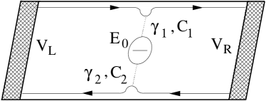
Figure 1: Sketch of a quantum dot coupled to chiral edge states via tunnel and capacitive couplings. The sample is driven out of equilibrium with an external bias $V_{L}=-V_{R}=V/2$.

For $B<0$ the chirality of the edge states is inverted and the nonequilibrium ($V_{L}\neq V_{R}$) polarization charge changes accordingly. Injected electrons in the upper (lower) edge state are now predominantly emitted from lead $R$ ($L$). Therefore, the rates now read $\Gamma_{L}^{+}=\gamma_{2}f(-B,V_{L})$, $\Gamma_{R}^{+}=\gamma_{1}f(-B,V_{R})$, $\Gamma_{L}^{-}=\gamma_{2}[1-f(-B,V_{L})]$ and $\Gamma_{R}^{-}=\gamma_{1}[1-f(-B,V_{R})]$, where $\mu_{d}(-B)=E_{0}-eC_{2}V_{L}/2C-eC_{1}V_{R}/2C$. We stress that the rates depend, quite generally, on the $B$ direction and differ for $C_{1}\neq C_{2}$. As demonstrated in Ref. san05, , the magnetoasymmetry of the polarization charge leads to a magnetoasymmetric addition energy of the quantum dot and, as a result, the current average is an uneven function of $B$. We can thus ask ourselves whether the current fluctuations also exhibit this effect.

Current fluctuations are characterized by the power spectrum, $S_{\alpha\beta}(\omega)$, of the current–current correlation function,bla00

$$S_{\alpha\beta}(\omega)=2\int e^{i\omega t}[\langle I_{\alpha}(t)I_{\beta}(0)\rangle-\langle I_{\alpha}\rangle\langle I_{\beta}\rangle]\,dt\,,$$ (2)

where $\langle I_{\alpha}\rangle$ is the averaged current across the $\alpha$ junction. Its stationary value can be found from the steady state solution of Eq. (1), which reads $\bar{p}_{0}=\Gamma^{-}/\Gamma$ and $\bar{p}_{1}=\Gamma^{+}/\Gamma$. As a consequence,

$$\langle I_{\alpha}\rangle=e[\Gamma_{\alpha}^{+}\bar{p}_{0}-\Gamma_{\alpha}^{-}\bar{p}_{1}]=e\frac{\Gamma_{\alpha}^{+}\Gamma^{-}-\Gamma_{\alpha}^{-}\Gamma^{+}}{\Gamma}\,,$$ (3)

where $\Gamma=\Gamma^{+}+\Gamma^{-}$.

The correlator $\langle I_{\alpha}(t)I_{\beta}(0)\rangle$ in Eq. (2) can be obtained from the conditional probability $p_{n,n^{\prime}}(t)$ that the state $n$ is occupied at time $t>0$ when the dot was in the state $n^{\prime}$ at $t=0$. Within our scheme the quantum regression theorem holds, and $p_{n,n^{\prime}}(t)$ obeys the same equations as $p_{n}(t)$. Hence, the eigenvalues of $\mathbf{M}$ completely determine the dynamical behavior of $p$. This can be seen from the noise expression $S_{\alpha\beta}=S_{\alpha}^{\rm Sch}\delta_{\alpha\beta}+S_{\alpha\beta}^{c}$, with $S_{\alpha}^{\rm Sch}$ the Schottky noise produced by correlated tunneling through a single junction and

$$S_{\alpha\beta}^{c}(\omega)=\sum_{\epsilon,\epsilon^{\prime}}\epsilon\epsilon^{\prime}\bar{p}_{\frac{1-\epsilon}{2}}[\Gamma_{\alpha}^{\epsilon^{\prime}}\Gamma_{\beta}^{\epsilon}+\Gamma_{\beta}^{\epsilon^{\prime}}\Gamma_{\alpha}^{\epsilon}]G_{\frac{1-\epsilon^{\prime}}{2},\epsilon}(\omega)\,,$$ (4)

where the “Green function” matrix for Eq. (1) reads,

$$\mathbf{G(\omega)}=-{\rm Re}(i\omega+\mathbf{M})^{-1}\,.$$ (5)

Care must be taken with the $\omega=0$ limit since $\mathbf{M}$ is singular. The matrix $\mathbf{M}$ has two eigenvalues, namely, $\lambda_{1}=0$ with an eigenvector given by the stationary solution $\vec{p}=(\Gamma^{-}/\Gamma\;\Gamma^{+}/\Gamma)^{T}$ and $\lambda_{2}=-\Gamma$, which describes a charge excitation in the system. Therefore, we can now use in Eq. (5) the spectral decomposition $\mathbf{M}=\sum_{i=1,2}\lambda_{i}\mathbf{U}\mathbf{E}_{i}\mathbf{U}^{-1}$, where $\mathbf{E}_{i}$ is a matrix with the element $(i,i)$ equal to 1 and the other elements are zeroes, the $i$-th column of $\mathbf{U}$ being the $i$-th eigenvector of $\mathbf{M}$. The $\lambda_{1}$ contribution cancels out the term $\langle I_{\alpha}\rangle\langle I_{\beta}\rangle$. As a result, $\mathbf{G}(\omega)=-\lambda_{2}\mathbf{U}\mathbf{E}_{2}\mathbf{U}^{-1}/(\omega^{2}+\lambda_{2}^{2})$ and we find the shot noise $S=-S_{LR}$ at $\omega=0$,

$$\frac{S}{2e^{2}}=\frac{(\Gamma_{L}^{+}\Gamma_{R}^{-}+\Gamma_{L}^{-}\Gamma_{R}^{+})\Gamma^{2}-2(\Gamma_{L}^{+}\Gamma_{R}^{-}-\Gamma_{L}^{-}\Gamma_{R}^{+})^{2}}{\Gamma^{3}}\,.$$ (6)

For $B>0$ and large bias such that $eV\gg E_{0},k_{B}T$, we have $\Gamma_{L}^{+}\approx\gamma_{1}$, $\Gamma_{L}^{-}\approx 0$, $\Gamma_{R}^{+}\approx 0$ and $\Gamma_{R}^{-}\approx\gamma_{2}$. Substituting these values in Eq. (6) we recover the double barrier case for noninteracting electrons, $S=2e^{2}\gamma_{1}\gamma_{2}(\gamma_{1}^{2}+\gamma_{2}^{2})/\gamma^{3}$, where $\gamma=\gamma_{1}+\gamma_{2}$.

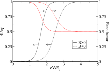
Figure 2: (Color online) Current (black curves) and Fano factor (red curves) as a function of bias voltage for $\gamma_{1}=\gamma_{2}=0.005E_{0}/\hbar$, $k_{B}T=0.1E_{0}$, $C_{1}=0.6$ and $C_{2}=0.4$.

III Results

Figure 2 shows results for the averaged current $I=\langle I_{L}\rangle=-\langle I_{R}\rangle$ and the Fano factor $F=S/2eI$ as a function of $V$. The current is exponentially suppressed at low $V$, increases at $V\sim CE_{0}/eC_{1}$ and reaches the limit value $e\gamma_{1}\gamma_{2}/\gamma$ for large voltages. When $B$ is reversed, the current now increases at $V\sim CE_{0}/eC_{2}$. Since we choose $C_{1}>C_{2}$ the $I(V,-B)$ is shifted to larger voltages compared to $I(V,+B)$. As a consequence, the differential conductance is generally $B$-asymmetric. The Fano factor is Poissonian at small $V$ since transport is dominated by thermal activated tunneling. For increasing $V$, the noise becomes sub-Poissonian and reaches saturation for large $V$. The crossover step from Poissonian noise to sub-Poissonian noise has a width which depends on $k_{B}T$. Like the current, the crossover center shifts to larger voltages when $B$ is reversed, thus yielding a magnetoasymmetric Fano factor.

Since the Fano factor depends on both the noise and the current and these are asymmetric under $B$ reversal, we plot in Fig. 3 the magnetic field asymmetry for the noise alone, which we define as $\Phi_{S}=[S(+B)-S(-B)]/2$. The asymmetry vanishes for small $V$, fulfilling the Onsager symmetry. At large $V$ the noise saturation value is independent of the $B$ direction since this limit corresponds to noninteracting fermions. As a result, the asymmetry vanishes. The asymmetry becomes maximal for intermediate voltages. Importantly, the asymmetry increases with the capacitance asymmetry, $\eta=(C_{1}-C_{2})/C$. Therefore, the current fluctuations are magnetoasymmetric only in the case where the electrostatic coupling of the dot with the edge states leads to an asymmetric screening of charges.

Figure 3: (Color online) Shot noise magnetoasymmetry for various capacitance asymmetries $\eta=(C_{1}-C_{2})/(C_{1}+C_{2})$. We take $\gamma_{1}=\gamma_{2}=0.005E_{0}/\hbar$ and $k_{B}T=0.1E_{0}$. Inset: Magnetoasymmetries of the leading-order nonlinear conductance and nonequilibrium noise at $V=0.03E_{0}/e$.

Furthermore, we consider the case of low voltages, $eV\ll k_{B}T$. Then, we can expand $I$ and $S$ in powers of $V$,

$$I = G_{1}V+G_{2}V^{2}+\mathcal{O}(V^{3})\,,$$ (7)

$$S = S_{0}+S_{1}V+\mathcal{O}(V^{2})\,.$$ (8)

We have checked that both the linear conductance $G_{1}$ and the equilibrium noise $S_{0}$ are even functions of $B$. They satisfy the linear fluctuation dissipation theorem, $S_{0}=4k_{B}TG_{1}$. While $G_{1}$ depends on the equilibrium potential in the dot, the nonlinear conductance term $G_{2}$ is, in general, a function of the screening electrostatic potential.christen This potential need not be $B$-symmetric.san04 Thus, the magnetoasymmetry $\Phi_{G_{2}}=[G_{2}(B)-G_{2}(-B)]/2$ acquires a finite value:

$$\Phi_{G_{2}}=\frac{e^{3}}{8}\frac{\gamma_{1}\gamma_{2}}{\gamma}\frac{\eta}{(k_{B}T)^{2}}{\rm sech}^{2}\frac{E_{0}}{2k_{B}T}\tanh\frac{E_{0}}{2k_{B}T}\,.$$ (9)

For high $k_{B}T$, Eq. (9) yields $\Phi_{G_{2}}=0$ since thermal fluctuations are $B$-symmetric. $\Phi_{G_{2}}$ determines the rate at which the current magnetoasymmetry increases with voltage, thus showing that magnetoasymmetries are a truly nonequilibrium effect.

The nonequilibrium noise at linear response [i.e., $S_{1}$ in Eq. (8)] is also $B$-asymmetric. To leading order in $V$, we find

$$\Phi_{S_{1}}=4k_{B}T\Phi_{G_{2}}\,,$$ (10)

where $\Phi_{S_{1}}=[S_{1}(B)-S_{1}(-B)]/2$. This is a relevant result of our work. Remarkably, we obtain the same functional dependence for the magnetoasymmetries of noise and current in the leading-order nonlinearities. We numerically confirm this prediction for a small value of $V$ (see inset of Fig. 3). This result can be related to the nonlinear fluctuation-dissipation theorem, which reads $S_{1}=4k_{B}TG_{2}$. It has been derived in Ref. tob07, for mesoscopic conductors at arbitrary voltages within the framework of full counting statistics. Thus, it is showntob07 that the nonlinear fluctuation-dissipation theorem holds even for interacting particles assuming time-reversibility (no magnetic fields). The nontrivial difference, however, is that in our theory microreversibility is broken due to the combined effect of magnetic fields and interactions san04 but still Eq. (10) holds. While detailed balance conditions are shown to hold far from equilibrium in the absence of magnetic fields,tob07 ; andr06 ; esp07 the same relations can not, generally, be established when microreversibility is broken.foe08 Despite this, we obtain an unexpected symmetry relation between the conductance and noise response magnetoasymmetries.

We note in passing that Eq. (10) is not a generalized of the fluctuation-dissipation theorem for which nonlinear fluctuations and the response are related via a (nontrivial) effective temperature, as in glassy systems, kob97 since the prefactor for both linear and nonlinear theorems is the same. Our result also differs from more general fluctuation theorems obeyed by full probability distributions.eva93

Figure 4: (Color online) Charge probability distribution magnetoasymmetry for $\gamma_{1}=\gamma_{2}=0.05E_{0}/\hbar$, $k_{B}T=0.4E_{0}$, $eV=-4.5E_{0}$, and various values of $\eta$. Inset: $P(N)$ for two field orientations and $\eta=0.4$.

To analyze higher-order terms one should consider fluctuations of the screening potential, which are beyond the scope of a mean-field approximation. Nevertheless, for classical Coulomb blockade effects the local potential fully screens the excess charges and quantum fluctuations are absent. Therefore, our model system is perfectly suitable for further extensions. We note that the Fano factor magnetoasymmetry, $\Phi_{F}=[F(B)-F(-B)]/2$, is quadratic in voltage:

$$\Phi_{F}=\frac{\gamma_{1}\gamma_{2}}{\gamma^{2}}\eta\left(\frac{eV}{2k_{B}T}\right)^{2}{\rm sech}^{2}\frac{E_{0}}{2k_{B}T}\tanh\frac{E_{0}}{2k_{B}T}\,.$$ (11)

A complete characterization of current fluctuations is given by the full counting statistics,lev93 which yields the entire probability distribution $P(N)$ of the transferred charge during the measurement time $t_{0}$. We follow the method of Bagrets and Nazarov bag03 to assess the cumulant generating function $\mathcal{S}(\chi)=-\ln\sum_{N}P(N)e^{iN\chi}$. Without loss of generality, we count charges in the $R$ lead. Therefore, we make the substitutions $\Gamma_{R}^{-}\to\Gamma_{R}^{-}e^{i\chi}$ and $\Gamma_{R}^{+}\to\Gamma_{R}^{+}e^{-i\chi}$ in the off-diagonal elements of $\mathbf{M}$ and $\mathcal{S}(\chi)$ is derived from $\mathcal{S}(\chi)=t_{0}\lambda_{2}(\chi)$. We calculate $P(N)$ within the saddle-point approximation, valid in the limit $t_{0}\to\infty$ bag03 and determine the magnetoasymmetry of $P(N)$. We show $\Phi_{P}=[P(N,+B)-P(N,-B)]/2$ in Fig. 4. $|\Phi_{P}|$ increases for increasing capacitance asymmetry and vanishes around $N\sim\gamma t_{0}/4$. This point corresponds to the mean current $\bar{I}=e\gamma/4$ for a dot symmetrically coupled ($\gamma_{1}=\gamma_{2}$) in the limit $eV\gg k_{B}T$.

IV Conclusions

To summarize, we have investigated magnetoasymmetric current fluctuations of a Coulomb-blockaded quantum dot. It is well established that the linear fluctuation-dissipation theorem makes an equivalence between linear-response functions to small perturbations and correlation functions describing fluctuations due to electric motion. In this work, we have found a similar fluctuation-dissipation relation that predicts an exact equivalence between the leading-order rectification and noise magnetoasymmetries, valid in the presence of external magnetic fields. Such relation has been very recently shown to derive from fundamental principles.foe08 Moreover, we have shown that the full probability distribution associated to the flow of charges is, generally, magnetic-field asymmetric. Since the effect studied here relies purely on interaction, it should be observable in many other systems exhibiting strong charging effects.

References

- (1) D. Sánchez and M. Büttiker, Phys. Rev. Lett. 93, 106802 (2004).
- (2) B. Spivak and A. Zyuzin, Phys. Rev. Lett. 93, 226801 (2004).
- (3) M. Büttiker and D. Sánchez, Int. J. Quantum Chem. 105, 906 (2005).
- (4) M.L. Polianski and M. Büttiker, Phys. Rev. Lett. 96, 156804 (2006).
- (5) A. De Martino, R. Egger, and A. M. Tsvelik, Phys. Rev. Lett. 97, 076402 (2006).
- (6) A.V. Andreev and L.I. Glazman, Phys. Rev. Lett. 97, 266806 (2006).
- (7) G.L.J.A. Rikken and P. Wyder, Phys. Rev. Lett. 94, 016601 (2005).
- (8) J. Wei, M. Schimogawa, Z. Whang, I. Radu, R. Dormaier, and D.H. Cobden, Phys. Rev. Lett. 95, 256601 (2005).
- (9) C. A. Marlow, R.P. Taylor, M. Fairbanks, I. Shorubalko, and H. Linke, Phys. Rev. Lett. 96, 116801 (2006).
- (10) R. Leturcq, D. Sánchez, G. Götz, T. Ihn, K. Ensslin, D.C. Driscoll, and A.C. Gossard, Phys. Rev. Lett. 96, 126801 (2006).
- (11) D. M. Zumbühl, C.M. Marcus, M.P. Hanson, and A.C. Gossard, Phys. Rev. Lett. 96, 206802 (2006).
- (12) L. Angers, E. Zakka-Bajjanni, R. Deblock, S. Guéron, H. Bouchiat, A. Cavanna, U. Gennser, and M. Polianksi, Phys. Rev. B 75, 115309 (2007).
- (13) D. Hartmann, L. Worschech, and A. Forchel, Phys. Rev. B 78, 113306 (2008).
- (14) L. Onsager, Phys. Rev. 38, 2265 (1931).
- (15) H.B.G. Casimir, Rev. Mod. Phys. 17, 343 (1945).
- (16) D. Sánchez and K. Kang, Phys. Rev. Lett. 100, 036806 (2008).
- (17) Ya.M. Blanter and M. Büttiker, Phys. Rep. 336, 1 (2000).
- (18) D. Loss and E.V. Sukhorukov, Phys. Rev. Lett. 84, 1035 (2000).
- (19) A. Cottet, W. Belzig, and C. Bruder, Phys. Rev. Lett. 92, 206801 (2004).
- (20) T. Novotný, A. Donarini, C. Flindt, and A.-P. Jauho, Phys. Rev. Lett. 92, 248302 (2004).
- (21) Y. Utsumi, D.S. Golubev, and G. Schön, Phys. Rev. Lett. 96, 086803 (2006).
- (22) G. Kießlich, E. Schöll, T. Brandes, F. Hohls, and R.J. Haug, Phys. Rev. Lett. 99, 206602 (2007).
- (23) For a recent review, see U.M.B. Marconi, A. Puglisi, L. Rondoni, and A. Vulpiani, Phys. Rep. 461, 111 (2008).
- (24) M. Büttiker, Phys. Rev. Lett. 57, 1761 (1986).
- (25) H. Förster and M. Büttiker, Phys. Rev. Lett. 101, 136805 (2008).
- (26) K. Saito and Y. Utsumi, Phys. Rev. B 78, 115429 (2008).
- (27) L.P. Kouwenhoven, C.M. Marcus, P.L. McEuen, S. Tarucha, R.M. Westervelt, and N.S. Wingreen, Proc. of the NATO ASI ”Mesoscopic Electron Transport”, edited by L.L. Sohn, L.P. Kouwenhoven and G. Schön (Kluwer Series E345, 1997), p. 105.
- (28) C.W.J. Beenakker, Phys. Rev. B 44, 1646 (1991); D. V. Averin, A. N. Korotkov, and K. K. Likharev, Phys. Rev. B 44, 6199 (1991); Y. Meir, N.S. Wingreen, and P.A. Lee, Phys. Rev. Lett. 66, 3048 (1991).
- (29) C.J.B. Ford, P.J. Simpson, I. Zailer, D.R. Mace, M. Yosefin, M. Pepper, D.A. Ritchie, J.E.F. Frost, M.P. Grimshaw, and G.A.C. Jones, Phys. Rev. B 49, 17456 (1994).
- (30) G. Kirczenow, A.S. Sachrajda, Y. Feng, R.P. Taylor, L. Henning, J. Wang, P. Zawadzki, and P.T. Coleridge, Phys. Rev. Lett. 72, 2069 (1994).
- (31) S. Hershfield, J.H. Davies, P. Hyldgaard, C.J. Stanton, and J.W. Wilkins, Phys. Rev. B 47, 1967 (1993).
- (32) U. Hanke, Yu.M. Galperin, K.A. Chao, and N. Zou, Phys. Rev. B 48, 17209 (1993).
- (33) A.N. Korotkov, Phys. Rev. B 49, 10381 (1994).
- (34) D. Sánchez and M. Büttiker, Phys. Rev. B 72, 201308 (2005).
- (35) T. Christen and M. Büttiker, Europhys. Lett. 35, 523 (1996).
- (36) T. Tobiska and Yu.V. Nazarov, Phys. Rev. B 72, 235328 (2005).
- (37) D. Andrieux and P. Gaspard, J. Stat. Mech. P01011 (2006).
- (38) M. Esposito, U. Harbola, and S. Mukamel, Phys. Rev. B 75, 155316 (2007).
- (39) W. Kob and J.L. Barrat, Phys. Rev. Lett. 78, 4581 (1997); G. Parisi, Phys. Rev. Lett. 79, 3660 (1997).
- (40) J.D. Evans, E.G.D. Cohen, and G.P. Morriss, Phys. Rev. Lett. 71, 2401 (1993); G. Gallavotti and E.G.D. Cohen, Phys. Rev. Lett. 74, 2694 (1995).
- (41) L.S. Levitov and G.B. Lesovik, JETP Lett. 58, 230 (1993).
- (42) D.A. Bagrets and Yu.V. Nazarov, Phys. Rev. B 67, 085316 (2003).