A Percolation-Theoretic Approach to Spin Glass Phase Transitions

Abstract

The magnetically ordered, low temperature phase of Ising ferro- magnets is manifested within the associated Fortuin-Kasteleyn (FK) random cluster representation by the occurrence of a single positive density percolating cluster. In this paper, we review our recent work on the percolation signature for Ising spin glass ordering — both in the short-range Edwards-Anderson (EA) and infinite-range Sherrington-Kirkpatrick (SK) models — within a two-replica FK representation and also in the different Chayes-Machta-Redner two-replica graphical representation. Numerical studies of the $\pm J$ EA model in dimension three and rigorous results for the SK model are consistent in supporting the conclusion that the signature of spin-glass order in these models is the existence of a single percolating cluster of maximal density normally coexisting with a second percolating cluster of lower density.

I Introduction

The question of whether laboratory spin glasses — or the theoretical models used to represent them — have a thermodynamic phase transition remains unresolved despite decades of work BY86 ; MPRRZ00 ; NSjpc03 . Although the infinite-range Sherrington-Kirkpatrick (SK) Ising spin glass is easily shown to possess a phase transition SK75 ; ALR87 , the existence of one in the corresponding short-range Edwards-Anderson (EA) EA75 Ising model (on the cubic lattice ${\bf Z}^{d}$) has not been established in any finite dimension. While some evidence for a transition has been uncovered through high-temperature expansions FS90 ; TH96 , analytical studies of variable long-range $1d$ models KAS83 , and extensive numerical simulations BY86 ; O85 ; OM85 ; KY96 , the issue remains unresolved MPR94 .

Random graph methods, and in particular the Fortuin-Kastelyn (FK) random cluster (RC) representation KF69 ; FK72 , provide a set of useful tools for studying phase transitions (more specifically, the presence of multiple Gibbs states arising from broken spin rotational symmetry) in discrete spin models. In these representations spin correlation functions can be expressed through the geometrical properties of associated random graphs. FK and related models are probably best known in the physics literature for providing the basis for powerful Monte Carlo methods for studying phase transitions Swe ; SwWa86 ; Wolff , but they have also proved important in obtaining rigorous results on phase transitions in discrete-spin ferromagnetic (including inhomogeneous and randomly diluted) models (e.g., ACCN87 ; IN88 ). Because of complications due to frustration, however, graphical representations have so far played a less important role in the study of spin glasses.

The goal of the studies presented here is to construct a viable approach which uses random graph methods to address the problem of phase transitions and broken symmetry in spin glass models. In earlier papers MNS07a ; MNS07b , we studied the “percolation signature” of spin glass ordering within two different graphical representations — the two-replica model of Chayes, Machta and Redner (CMR) CMR98 ; CRM98 and a two-replica version of the FK representation (TRFK), as proposed in Sec. 4.1 of NS07 . The purpose of that analysis was to show that FK methods could be utilized to study spin glass phase transitions. The result of this work was the uncovering of strong evidence that the existence of a spin glass transition coincides with the emergence of doubly percolating clusters of unequal densities. This scenario is more complex than what occurs in ferromagnetic models, where the phase transition coincides with percolation of a single FK cluster.

In what follows, we first review the FK random cluster representation for ferromagnetic models, and then describe our analytical and numerical results for spin glasses.

II The Fortuin-Kasteleyn Random Cluster Representation

In this section we briefly review the Fortuin-Kasteleyn random cluster representation KF69 ; FK72 which relates the statistical mechanics of Ising (or Potts) models to a dependent percolation problem. Our focus will be on Ising models throughout, but the analysis is easily extended to more general Potts models.

II.1 Ferromagnetic Models

We start by considering a nearest-neighbor Ising ferromagnet, whose couplings $J_{xy}\geq 0$ are not necesarily identical:

$${\cal H}=-\sum_{\langle xy\rangle}J_{xy}\sigma_{x}\sigma_{y}\ ,$$ (1)

where, as already noted, $J_{xy}\geq 0$ and the sum is over nearest neighbor pairs of sites in ${\bf Z}^{d}$. Each such coupling is associated with an edge, or bond, $\langle x,y\rangle$, with the set of all such bonds denoted ${\bf E}^{d}$.

The RC approach introduces parameters $p_{xy}\in[0,1)$ through the formula:

$${\cal P}_{xy}=1-\exp[-2\beta|J_{xy}|]\,,$$ (2)

where $\beta$ is the inverse temperature. One can then define a probability measure $\mu_{\rm RC}$ on $\{0,1\}^{{\bf E}^{d}}$, that is, on 0- or 1-valued bond occupation variables $\omega_{xy}$. It is one of two marginal distributions (the other being the ordinary Gibbs distribution) of a joint distribution on $\Omega=\{-1,+1\}^{{\bf Z}^{d}}\times\{0,1\}^{{\bf E}^{d}}$ of the spins and bonds together (such a joint distribution will be introduced in Sec. II.3). The marginal distribution $\mu_{\rm RC}$ is given formally by

$$\mu_{\rm RC}(\{\omega_{xy}\})=Z_{\rm RC}^{-1}\ 2^{\#(\{\omega_{xy}\})}\ \mu_{\rm ind}(\{\omega_{xy}\})\ 1_{U}(\{\omega_{xy}\})\,,$$ (3)

where $Z_{\rm RC}$ is a normalization constant, $\#(\{\omega_{xy}\})$ is the number of clusters determined by the realization $\{\omega_{xy}\}$, $\mu_{\rm ind}(\{\omega_{xy}\})$ is the Bernoulli product measure corresponding to independent occupation variables with $\mu_{\rm ind}(\{\omega_{xy}=1\})={\cal P}_{xy}$, and $1_{U}$ is the indicator function on the event $U$ in $\{0,1\}^{{\bf E}^{d}}$ that there exists a choice of the spins $\{\sigma_{x}\}$ so that $J_{xy}\omega_{xy}\sigma_{x}\sigma_{y}\geq 0$ for all $\langle x,y\rangle$ WaSw88 ; KO88 ; N93 .

There are several things to be noted about (3). The factor 2 in the term $2^{\#(\{\omega_{xy}\})}$ arises because we’ve confined ourselves to Ising models, so that every connected cluster of spins (each such connected cluster consists of all satisified bonds) can be in one of two states (in the ferromagnetic case, all up or all down); in a $q$-state Potts model, this term would then be replaced by $q^{\#(\{\omega_{xy}\})}$. More importantly, the indicator function on $U$, which is the event that there is no frustration in the occupied bond configuration, is always one for the ferromagnet; consequently, this term is superfluous for ferromagnetic models. We include it, however, because it will be needed when we generalize to models with frustration. Finally, we note that finite-volume versions of the above formulas, with specified boundary conditions, can be similarly constructed.

In the case of a ferromagnet, there are general theorems BK89 which ensure that when percolation occurs, there is a unique percolating cluster. It then easily follows that RC percolation within the FK representation (or “FK percolation” for short) corresponds to the presence of multiple Gibbs states (in the ferromagnet, magnetization up and magnetization down), and moreover that the onset of percolation occurs at the ferromagnetic critical temperature. To prove this, it is sufficient to show that FK percolation is both necessary and sufficient for the breaking of global spin flip symmetry in the ferromagnet. To see that FK percolation is a necessary condition, note that the contribution to the expectation of $\sigma_{0}$ from any finite RC cluster is zero: if a spin configuration $\sigma$ is consistent with a given RC bond realization within such a cluster, so is $-\sigma$, and both will be equally likely. As a consequence, $\langle\sigma_{0}\rangle=0$ in infinite volume in the absence of RC percolation.

To see that RC percolation is a sufficient condition for the magnetization order parameter to be nonzero, consider a finite volume $\Lambda_{L}$ with fixed boundary conditions, i.e., a specification $\overline{\sigma}_{x}=\pm 1$ for each $\overline{\sigma}_{x}\in\partial\Lambda_{L}$. For the ferromagnet, by first choosing all $\overline{\sigma}_{x}=+1$ and then all $\overline{\sigma}_{x}=-1$, one can change the sign of the spin $\sigma_{0}$ at the origin even as $L\to\infty$. That is, boundary conditions infinitely far away affect $\sigma_{0}$, which is a signature of the existence of multiple Gibbs states.

When attention is confined to ferromagnetic models, the mapping of the FK formalism to interesting statistical mechanical quantities is straightforward (and intuitive); for example

$$\langle\sigma_{x}\sigma_{y}\rangle=\mu_{\rm RC}(x\leftrightarrow y)\,,$$ (4)

where $\langle\sigma_{x}\sigma_{y}\rangle$ is the usual Gibbs two-point correlation function and $\mu_{\rm RC}(x\leftrightarrow y)$ is the RC probability that $x$ and $y$ are in the same cluster. Similarly, with “wired” boundary conditions (i.e., each boundary spin is connected to its nieghbors), one has

$$\langle\sigma_{x}\rangle_{+}=\mu_{\rm RC}(x\leftrightarrow\infty)\,.$$ (5)

So for ferromagnets, a phase transition from a unique (paramagnetic) phase at low $\beta$ to multiple infinite-volume Gibbs states at large $\beta$ is equivalent to a percolation phase transition for the corresponding RC measure.

II.2 Spin Glass Models; The TRFK Representation

For spin glasses (or other nonferromagnets with frustration) the situation is more complicated. Now for two sites $x$ and $y$, (4) becomes

$$\langle\sigma_{x}\sigma_{y}\rangle=\langle 1_{x\leftrightarrow y}\eta(x,y)\rangle_{RC};\,\,\,\eta(x,y)=\prod_{\langle x^{\prime}y^{\prime}\rangle\in{\cal C}}{\rm sgn}(J_{x^{\prime}y^{\prime}})\,,$$ (6)

where ${\cal C}$ is any path of occupied bonds from $x$ to $y$. By the definition of $U$, any two such paths ${\cal C}$ and ${\cal C^{\prime}}$ in the same cluster will satisfy $\prod_{\langle x^{\prime}y^{\prime}\rangle\in{\cal C}}{\rm sgn}(J_{x^{\prime}y^{\prime}})=\prod_{\langle x^{\prime}y^{\prime}\rangle\in{\cal C^{\prime}}}{\rm sgn}(J_{x^{\prime}y^{\prime}})$.

Just as in the ferromagnet, if percolation of a random cluster occurs in the FK representation, the percolating cluster is unique (in each realization of FK spins and bonds) NS07 ; GKN92 . In spite of this, RC percolation alone is no longer sufficient to prove broken spin-flip symmetry in the EA spin glass. This is because even in the presence of RC percolation, it is unclear whether there exist any two sets of boundary conditions that can alter the state of the spin at the origin from arbitrarily far away. Although the infinite cluster in any one RC realization is unique, different RC realizations can have different paths from $0\leftrightarrow\partial\Lambda_{L}$, and because of frustration this can lead to different signs for $\sigma_{0}$. So percolation might still allow for $\langle\sigma_{0}\rangle\to 0$ as $L\to\infty$, independently of boundary condition.

Indeed, it is known that FK bonds percolate well above the spin glass transition temperature. For the three-dimensional Ising spin glass on the cubic lattice, Fortuin-Kasteleyn bonds percolate at $\beta_{{\rm FK},p}\approx 0.26$ ArCoPe91 while the inverse critical temperature is believed to be $\beta_{c}=0.89\pm 0.03$ KaKoYo06 . Near the spin glass critical temperature, the giant FK cluster includes most of the sites of the system. For this reason, the Swendsen-Wang algorithm, though valid, is inefficient for simulating spin glasses.

However, it is an open question as to whether the presence of “single ” (see below) FK percolation would lead to a slower, e.g. power-law, decay of correlation functions even though the Gibbs state is unique. If this were to happen, then the onset of single FK percolation would imply a phase transition in the spin glass, though not multiple Gibbs states and hence no broken spin-flip symmetry. This possibility was suggested in NS07 ; but to date, no evidence exists to support it.

Nonetheless, single FK percolation remains a necessary condition for multiple (symmetry-broken) Gibbs phases in the spin glass, for the same reason as for the ferromagnet. A slightly stronger version of that argument N93 proves that the transition temperature for an EA spin glass, if it exists, is bounded from above by the transition temperature in the corresponding (disordered) ferromagnet.

The essential difference (from the point of view of FK percolation) between the ferromagnet and the spin glass is the factor $1_{U}$ in (3). It is somewhat easier to discuss this factor in the context of finite volumes. Let $\Lambda_{L}$ denote the $L^{d}$ cube centered at the origin, and let $\hat{\Lambda}_{L}$ denote the set of bonds $b=\langle x,y\rangle$ with both $x$ and $y$ in $\Lambda_{L}$. For models containing frustration, $U$ is typically not all of $\{0,1\}^{\hat{\Lambda}_{L}}$, unlike for the ferromagnet; it is the set of all unfrustrated bond configurations (so that the product of couplings around any closed loop in such a configuration is always positive).

So is there a way to extend the above considerations to arrive at a sufficient condition for multiple Gibbs states in spin glass models? We begin by noting that FK clusters identify magnetization correlations; but spin glass ordering is manifested by the Edwards-Anderson (EA) order parameter, and not the magnetization, becoming nonzero. The EA order parameter $q_{EA}$ can be defined with respect to two independent replicas of the system, each with the same couplings $\{J_{xy}\}$. Denoting the spins in the two replicas by $\{\sigma_{x}\}$ and $\{\tau_{x}\}$, each taking values $\pm 1$, $q_{EA}$ is defined in terms of the overlap,

$$Q\,=\,N^{\,-1}\sum_{\{x\}}\sigma_{x}\tau_{x}\ ,$$ (7)

in the limit as the number of sites $N\to\infty$. In general, $Q$ is a random variable whose maximum possible value is $q_{EA}$, but in the case where (in the limit $N\to\infty$) $\{\sigma_{x}\}$ and $\{\tau_{x}\}$ are drawn from a single pure state, $Q$ takes on only the single value $q_{EA}$.

Using this as a guide, it appears that one possibility, proposed in MNS07a ; MNS07b ; NS07 , for extending FK methods to spin glasses is to use what might be called double FK percolation. Here one expands the sample space $\Omega$ to include two independent copies of the bond occupation variables (for a given ${\cal J}$ configuration), and defines the variable $r_{xy}=\omega_{xy}\omega^{\prime}_{xy}$, where $\omega_{xy}$ and $\omega^{\prime}_{xy}$ are taken from the two copies. One then replaces percolation of $\{\omega_{xy}\}$ in the single RC case with percolation of $\{r_{xy}\}$. It is not hard to see that this would be a sufficient condition for the existence of multiple Gibbs phases (and consequently, for a phase transition).

This is not the only way, however, to use “double” percolation of RC clusters in some form to arrive at a condition for spin glass ordering; the above describes what we denoted in the Introduction as the TRFK approach. In the next subsection we present a closely related approach, the CRM two-replica graphical representation, which requires a more lengthy description. Once this is done, we will discuss how both representations can be used to illuminate the nature of phase transitions in short-range spin glass models.

II.3 The CMR Representation

In describing these “double FK” representations, we will find it useful to reformulate our description of the relevant measures slightly using a joint spin-bond distribution introduced by Edwards and Sokal ES88 . The statistical weight ${\cal W}$ for the Edwards-Sokal distribution on a finite lattice $\Lambda_{L}$ is

$${\cal W}(\{\sigma_{x}\},\{\omega_{xy}\};p)=p^{|\omega|}(1-p)^{N_{b}-|\omega|}\Delta(\{\sigma_{x}\},\{\omega_{xy}\})\,.$$ (8)

Here $|\omega|=\sum_{\langle x,y\rangle}\omega_{xy}$ is the number of occupied bonds and $N_{b}$ is the total number of bonds on the lattice. The factor $\Delta(\{\sigma_{x}\},\{\omega_{xy}\})$ is introduced to require that every occupied bond is satisfied; it is defined by

$$\Delta(\{\sigma_{x}\},\{\omega_{xy}\})=\left\{\begin{array}[]{l}1\mbox{ if for every $xy$: }\omega_{xy}\sigma_{x}\sigma_{y}\geq 0\\ 0\mbox{ otherwise}\,.\end{array}\right.$$ (9)

With $p$ defined as in (2) and with all $J_{xy}=J>0$, it is easy to verify that the spin and bond marginals of the Edwards-Sokal distribution are the ferromagnetic Ising model with coupling strength $J$ and the Fortuin-Kasteleyn random cluster model (cf. (3)), respectively.

We can now adapt the above representation to the $\pm J$ Ising spin glass. (With minor modifications, it can also be adapted to Gaussian and other distributions for the couplings.) The corresponding Edwards-Sokal weight is the same as that given in Eq. (8). The $\Delta$ factor must still enforce the rule that all occupied bonds are satisfied,

$$\Delta(\{\sigma_{x}\},\{\omega_{xy}\};\{J_{xy}\})=\left\{\begin{array}[]{l}1\mbox{ if for every $xy$: }J_{xy}\omega_{xy}\sigma_{x}\sigma_{y}\geq 0\\ 0\mbox{ otherwise}\,.\end{array}\right.$$ (10)

so (cf. (3)) $1_{U}=\max_{\{\sigma_{x}\}}\Delta(\{\sigma_{x}\},\{\omega_{xy}\};\{J_{xy}\})$. The spin marginal of the corresponding Edwards-Sokal distribution is now the Ising spin glass with couplings $\{J_{xy}\}$. But the relationship between spin-spin correlations and bond connectivity is complicated by the presence of antiferromagnetic bonds. Now one has

$$\langle\sigma_{x}\sigma_{y}\rangle=$$ (11)

$$\mbox{Prob}\{x\mbox{ and} y\mbox{ connected by even number of antiferromagnetic bonds}\}$$

$$-\mbox{Prob}\{x\mbox{ and} y\mbox{ connected by odd number of antiferromagnetic bonds}\}.$$

The two-replica CMR graphical representation, introduced in CMR98 ; CRM98 , incorporates, in addition to the spin variables $\{\sigma_{x}\}$ and $\{\tau_{x}\}$, two sets of bond variables $\{\omega_{xy}\}$ and $\{\eta_{xy}\}$, each taking values in $\{0,1\}$. Now the Edwards-Sokal weight is

$${\cal W}(\{\sigma_{x}\},\{\tau_{x}\},\{\omega_{xy}\},\{\eta_{xy}\};\{J_{xy}\})\\ =B_{\rm blue}(\{\omega_{xy}\})B_{\rm red}(\{\eta_{xy}\})\Delta(\{\sigma_{x}\},\{\tau_{x}\},\{\omega_{xy}\};\{J_{xy}\})\Gamma(\{\sigma_{x}\},\{\tau_{x}\},\{\eta_{xy}\})$$ (12)

where the $B$’s are Bernoulli factors for the two types of bonds,

$$B_{\rm blue}(\{\omega_{xy}\})={\cal P}_{\rm blue}^{|\omega|}(1-{\cal P}_{\rm blue})^{N_{b}-|\omega|}$$ (13)

$$B_{\rm red}(\{\eta_{xy}\})={\cal P}_{\rm red}^{|\eta|}(1-{\cal P}_{\rm red})^{N_{b}-|\eta|}$$ (14)

and the bond occupation probabilities are

$${\cal P}_{\rm blue} = 1-\exp(-4\beta|J|)$$ (15)

$${\cal P}_{\rm red} = 1-\exp(-2\beta|J|).$$ (16)

So $B_{\rm blue}(\{\omega_{xy}\})=\mu_{\rm ind}(\{\omega_{xy}\})$. The $\Delta$ and $\Gamma$ factors constrain where the two types of occupied bonds are allowed,

$$\Delta(\{\sigma_{x}\},\{\tau_{x}\},\{\omega_{xy}\};\{J_{xy}\})$$ (19)

$$= \left\{\begin{array}[]{l}1\mbox{ if for every $xy$: }J_{xy}\omega_{xy}\sigma_{x}\sigma_{y}\geq 0\mbox{ and }J_{xy}\omega_{xy}\tau_{x}\tau_{y}\geq 0\\ 0\mbox{ otherwise}\,,\end{array}\right.$$

$$\Gamma(\{\sigma_{x}\},\{\tau_{x}\},\{\eta_{xy}\})$$ (22)

$$= \left\{\begin{array}[]{l}1\mbox{ if for every $xy$: }\eta_{xy}\sigma_{x}\sigma_{y}\tau_{x}\tau_{y}\leq 0\\ 0\mbox{ otherwise}\,.\end{array}\right.$$

We refer to the $\omega$-occupied bonds as “blue” and the $\eta$-occupied bonds as “red”. The $\Delta$ constraint says that blue bonds are allowed only if the bond is satisfied in both replicas. The $\Gamma$ constraint says that red bonds are allowed only if the bond is satisfied in exactly one replica.

It is straightforward to verify that the spin marginal of the two-replica Edwards-Sokal weight is that for two independent Ising spin glasses with the same couplings,

$$\sum_{\{\omega\}\{\eta\}}{\cal W}(\{\sigma_{x}\},\{\tau_{x}\},\{\omega_{xy}\},\{\eta_{xy}\};\{J_{xy}\})=\mbox{const}\times\exp\left[\beta\sum_{\langle xy\rangle}J_{xy}(\sigma_{x}\sigma_{y}+\tau_{x}\tau_{y})\right]$$ (23)

Connectivity by occupied bonds in the two-replica representation is related to correlations of the local spin glass order parameter,

$$Q_{x}=\sigma_{x}\tau_{x}.$$ (24)

It is straightforward to verify that

$$\langle Q_{x}Q_{y}\rangle=\mbox{Prob}\{x\mbox{ and }y\mbox{ connected by even number of red bonds}\}$$ (25)

$$-\mbox{Prob}\{x\mbox{ and }y\mbox{ connected by odd number of red bonds}\}.$$

As in the case of the FK representation, a minus sign complicates the relationship between correlations and connectivity but in a conceptually different way. The second term in Eq. (25) is independent of the underlying couplings in the model and is present for both spin glasses and ferromagnetic models.

As noted earlier, for ferromagnets (in the absence of non-translation-invariant boundary conditions), the signature of ordering is a single percolating FK cluster. For spin glasses, the situation is more complicated as there can be more than one percolating cluster. However, if the CMR graphical representation displays a single percolating blue cluster of largest density, one can similarly show broken symmetry, for either EA or SK models. This is because one can impose “agree” or “disagree” boundary conditions between those $\sigma_{x}$ and $\tau_{x}$ boundary spins belonging to the maximum density blue network. In the infinite volume limit, these two boundary conditions give different Gibbs states for the $\sigma$-spin system (for fixed $\tau$) related to each other by a global spin flip (of $\sigma$).

It is a separate matter, however, to relate in a simple way the EA order parameter to the density difference in blue (or more generally, doubly percolating) clusters. Intuitively, it seems that there should be a simple correspondence, and in fact such a relation is easy to show for the SK model: here the overlap $Q$ is exactly the difference in density between two percolating blue clusters MNS07a . But it is not immediately obvious that a similar density difference can be simply related to the EA order parameter (although the arguments above imply that here also a density difference implies a nonzero $Q$.) This is because in a two-replica situation, it is not immediately obvious that there is no contribution from finite clusters in short-range models.

For the TRFK representation, similar reasoning shows that the occurrence of exactly two doubly-occupied percolating FK clusters with different densities implies broken symmetry for the spin system NS07 and that $Q$ should equal (and once again, does equal in the SK model) the density difference. In MNS07a we presented preliminary numerical evidence that there is such a nonzero density difference below the spin glass transition temperature for the $d=3$ EA $\pm J$ spin glass (for both the TRFK and CMR representations). We will discuss these results further in Sec. IV. But now we turn to a review of some rigorous results, particularly for the SK model, that appeared in MNS07a and MNS07b .

III Rigorous Results

The SK model permits a fairly extensive rigorous analysis of both the CMR and TRFK representations which, when combined with other known results, permits a sharp picture to emerge of the connection between double FK percolation (we use this more general term to refer to any representation that relies on two FK replicas, such as CMR or TRFK), and a phase transition to a low-temperature spin glass phase with broken spin-flip symmetry. The surprising feature to emerge from this analysis is that in the CMR representation, there already exist well above the transition temperature two percolating networks of blue bonds, of equal density and in all respects macroscopically indistinguishable. Below the critical temperature $T_{c}$, the indistinguishability is lifted: the two infinite clusters assume different densities.

On the other hand, there is no double FK percolation at all above $T_{c}$ in the TRFK representation, but below $T_{c}$ there are again two percolating double clusters of unequal density.

We do not yet know whether this difference in the two pictures above $T_{c}$ persists in the EA model, but numerical evidence (to be discussed in the next section) so far appears to indicate that it does not: in the EA spin glass, both representations seem to behave similarly to CMR in the SK model.

The SK Hamiltonian for an $N$-spin system is

$${\cal H}_{N}=-{\frac{1}{\sqrt{N}}}\sum_{1\leq i<j\leq N}J_{ij}\sigma_{i}\sigma_{j}\ ,$$ (26)

where $i,j=1,\ldots N$ are vertices on a complete graph. The couplings $J_{ij}$ are i.i.d. random variables chosen from a probability measure $\rho$ satisfying the following properties:

1) The distribution is symmetric: $\rho(u)=\rho(-u)$.

2) $\rho$ has no $\delta$-function at $u=0$.

3) The moment generating function is finite: $\int_{-\infty}^{\infty}d\rho(u)\ e^{-t|u|}<\infty$ for all real $t$.

4) The second moment of $\rho$ is finite; we normalize it to one: $\int_{-\infty}^{\infty}d\rho(u)\ u^{2}=1$.

So the results of this section hold for Gaussian and many other distributions (although not diluted ones, because of requirement (2)), but the analysis is simplest for the $\pm J$ model, to which we confine our attention for the remainder of this section. We therefore assume that $J_{ij}=\pm 1$ with equal probability; for this distribution (or any other satisfying property (3)) $\beta_{c}=1$ BY86 ; SK75 .

It is relatively easy to see, using a heuristic argument presented in MNS07a , at what temperature a single FK cluster will form. The SK energy per spin, $u$, is given above the critical temperature by $u=-\beta/2$. Therefore, for large $N$ the fraction $f_{s}$ of satisfied edges is

$$f_{s}\sim\frac{1}{2}-uN^{-1/2}\ .$$ (27)

From (2) it follows that a fraction ${\cal P}_{\rm FK}=1-\exp(-2\beta N^{-1/2})\approx 2\beta N^{-1/2}$ of satisfied edges are occupied. According to the theory of random graphs (see Bollobas01 ), a giant cluster forms in a random graph of $N$ vertices when a fraction $x/N$ of edges is occupied with $x>1$, and there is then a single giant cluster ER60 . So if edges are satisfied independently (which of course they’re not — this is why this argument is heuristic only), then single replica FK giant clusters should form when $\beta=xN^{-1/2}$ when $x>1$. The single replica FK percolation threshold is therefore at

$$\beta_{{\rm FK},p}=N^{-1/2}\,,$$ (28)

and above this threshold, there should be a single giant FK cluster.

This simple argument can be made rigorous NS07 , but the basic ideas are already displayed above. The rigorous argument obtains upper and lower bounds for the conditional probability that an edge $\{x_{0}y_{0}\}$ is satisfied, given the satisfaction status of all the other edges. If these bounds are close to each other (for large $N$) then treating the satisfied edges as though chosen independently can be justified. We now describe that argument.

To avoid the problem of non-independence of satisfied edges, we fix all couplings $J_{xy}$ but one, which we denote $J_{x_{0}y_{0}}$, and ask for the conditional probability of its sign given the configuration of all other couplings and all spins $\sigma_{x}$. The ratio $Z_{+}/Z_{-}$ of the partition functions with $J_{x_{0}y_{0}}=+N^{-1/2}$ and $J_{x_{0}y_{0}}=-N^{-1/2}$ satisfies

$$\exp(-2\beta N^{-1/2})\,\leq\,|Z_{+}/Z_{-}|\,\leq\exp(2\beta N^{-1/2})\,.$$ (29)

The conditional probabilities $P_{\pm}$ that $J_{x_{0}y_{0}}=\pm N^{-1/2}$ therefore satisfy

$$e^{-4\beta/\sqrt{N}}\leq e^{-2\beta/\sqrt{N}}|Z_{-}/Z_{+}|\leq P_{+}/P_{-}\leq e^{2\beta/\sqrt{N}}|Z_{-}/Z_{+}|\leq e^{4\beta/\sqrt{N}}\,.$$ (30)

Let $P_{s}$ ($P_{u}$) be the conditional probability for any edge $\{x_{0}y_{0}\}$ to be satisfied (unsatisfied) given the satisfaction status of all other edges. These must then be bounded as follows:

$$e^{-4\beta/\sqrt{N}}\leq P_{s}/P_{u}\leq e^{4\beta/\sqrt{N}}\,,$$ (31)

and therefore

$$\frac{1}{2}-{\mathrm{O}}(\beta/\sqrt{N})=(e^{4\beta/\sqrt{N}}+1)^{-1}\leq P_{s}\leq(e^{-4\beta/\sqrt{N}}+1)^{-1}=\frac{1}{2}+{\mathrm{O}}(\beta/\sqrt{N})\,.$$ (32)

One now obtains rigorously the same conclusions as before — i.e., (28) is valid with a single giant FK cluster for $\beta=\beta_{N}\geq xN^{-1/2}$ with any $x>1$.

Essentially the same argument is used for the more interesting case of double percolation. Here there are two spin replicas denoted by $\sigma$ and $\tau$. We are now interested in percolation of doubly satisfied edges; the spins at the vertices of each such edge must satisfy $\sigma_{x}\tau_{x}=\sigma_{y}\tau_{y}$ (and then will be satisifed for exactly one of the two signs of $J_{xy}$). We note an immediate difference between the CMR and TRFK representations: for the former, doubly satisfied edges are occupied with probability ${\cal P}_{\rm CMR}=1-\exp(-4\beta N^{-1/2})\sim 4\beta N^{-1/2}$, while for the latter, ${\cal P}_{\rm TRFK}=[1-\exp(-2\beta N^{-1/2})]^{2}\sim 4\beta^{2}/N$. It seems likely that this difference occurs only for the SK model; the various factors of $N$ are absent in the EA model.

We can proceed much as in the single-replica case by dividing all $(\sigma,\tau)$ configurations into two sectors — the agree (where $\sigma_{x}=\tau_{x}$) and the disagree sectors (where $\sigma_{x}=-\tau_{x}$). We also denote by $N_{a}$ and $N_{d}$ the numbers of sites in the sectors and denote by $D_{a}=N_{a}/N$ and $D_{d}=N_{d}/N$ the sector densities (so that $D_{a}+D_{d}=1$). The spin overlap $Q$ is then just

$$Q=\frac{1}{N}\sum_{x}\sigma_{x}\tau_{x}=\frac{N_{a}-N_{d}}{N}=D_{a}-D_{d}\,.$$ (33)

For $\beta\leq\beta_{c}=1$, $Q\to 0$ as $N\to\infty$ (because the EA order parameter is zero in the paramagnetic phase) while for $\beta>\beta_{c}=1$, $\overline{\langle Q^{2}\rangle}>0$ as $N\to\infty$, where $\overline{(\cdot)}$ denotes an average over couplings. So it must be that $D_{a}=D_{d}$ for $\beta\leq 1$ while $D_{a}\neq D_{d}$ for $\beta>1$.

The arguments for the single replica case can be repeated separately within the agree and disagree sectors. Letting $\bar{P}_{\pm}$ denote the conditional probabilities that $J_{x_{0}y_{0}}=\pm N^{-1/2}$ given the other $J_{xy}$’s and all $\sigma_{x}$’s and $\tau_{x}$’s, we have within either of the two sectors that

$$e^{-8\beta/\sqrt{N}}\leq e^{-4\beta/\sqrt{N}}|Z_{-}/Z_{+}|^{2}\leq{\bar{P}_{+}}/{\bar{P}_{-}}\leq e^{4\beta/\sqrt{N}}|Z_{-}/Z_{+}|^{2}\leq e^{8\beta/\sqrt{N}}$$ (34)

so that the conditional probability within a single sector $P_{ds}$ for ${x_{0}y_{0}}$ to be doubly satisfied is $(1/2)+{\mathrm{O}}(\beta N^{-1/2})$. For $\beta\leq\beta_{c}$, we have $D_{a}=1/2$, $D_{d}=1/2$ (in the limit $N\to\infty$) and so in either sector, double FK percolation is approximately a random graph model with $N/2$ sites and bond occupation probability $(1/2)4\beta^{2}N^{-1}=\beta^{2}(N/2)^{-1}$; thus double FK giant clusters do not occur for $\beta^{2}\leq 1$ in the TRFK representation.

In the CMR representation, blue percolation corresponds to bond occupation probability $(1/2)4\beta N^{-1/2}$ $=\beta N^{1/2}(N/2)^{-1}$ and so the threshold for blue percolation is given by $\beta_{{\rm CMR},p}=N^{-1/2}$. But now there are two giant clusters, one in each of the two sectors, and as noted above they satisfy $D_{a}=D_{d}$ when $\beta\leq\beta_{c}=1$. For $\beta>\beta_{c}$, $D_{a}\neq D_{d}$. Since $\beta N^{1/2}\to\infty$ for $\beta>\beta_{c}$ (indeed for any fixed $\beta>0$), it follows from random graph theory that each giant cluster occupies the entire sector so that $D_{a}$ and $D_{d}$ are also the cluster percolation densities of the two giant clusters.

In the case of two-replica FK percolation for $\beta>\beta_{c}$, let us denote by $D_{max}$ and $D_{min}$ the larger and smaller of $D_{a}$ and $D_{d}$, so that $D_{max}+D_{min}=1$ and $D_{max}-D_{min}=Q$. Then for $\beta>\beta_{c}$, the bond occupation probability in the larger sector is $\beta^{2}(N/2)^{-1}=2\beta^{2}D_{max}(D_{max}N)^{-1}$ with $2\beta^{2}D_{max}>1$ and there is a (single) giant cluster in that larger sector. There will be another giant cluster (of lower density) in the smaller sector providing $2\beta^{2}D_{min}=\beta^{2}(1-Q)>1$. Since $Q\leq q_{EA}$, for this to be the case it suffices if for $\beta>\beta_{c}$,

$$q_{EA}<1-\frac{1}{\beta^{2}}\ .$$ (35)

The estimated behavior of $q_{EA}$ both as $\beta\to 1+$ and as $\beta\to\infty$ BY86 suggests that this is always valid. In any case, we have rigorously proved that there is a unique maximal density double FK cluster for $\beta>\beta_{c}$.

An important feature of spin glass order is ultrametricity, which is believed to be true at least for the SK model MPSTV84 , although it has not yet been proved rigorously. For the spin overlaps coming from three replicas put into rank order, $Q_{(1)}\geq Q_{(2)}\geq Q_{(3)}$, ultrametricity is the property that $Q_{(2)}=Q_{(3)}$. The issue of percolation signatures for ultrametricity in the SK model is treated at length in MNS07b . We only mention here one of those signatures, which concerns the four percolating clusters that arise in a CMR representation of three replicas when considering bonds that are simultaneously blue both for replicas one and two as well as for replicas one and three. Denoting the four cluster densities in rank order as $x_{(1)}\geq x_{(2)}\geq x_{(3)}\geq x_{(4)}$, the percolation version of the ultrametric property is that $x_{(1)}>x_{(2)}$ and $x_{(3)}=x_{(4)}$. The case $x_{(2)}=x_{(3)}$ (resp., $x_{(2)}>x_{(3)}$) corresponds to $Q_{(1)}>Q_{(2)}$ (resp, $Q_{(1)}=Q_{(2)}$). See  MNS07b for more details.

IV Numerical Methods and Results

We have carried out numerical simulations to explore the properties of two-replica FK representations described in the previous sections for the case of the three-dimensional $\pm J$ EA spin glass. The Monte Carlo algorithm that we use also makes use of the CMR representation in addition to parallel tempering and Metropolis sweeps. Similar methods have been previously applied by Swendsen and Wang SwWa86 ; WaSw88 ; WaSw05 and others Houdayer01 ; jorg05 ; jorg06 . The algorithm is described in more detail in MNS07a , here we provide some additional details about the CMR component of the algorithm. The CMR cluster algorithm alternates between “bond moves” and “spin moves.” The bond move takes a pair of EA spin configurations $\{\sigma_{x}\}$ and $\{\tau_{x}\}$, both in the same realization of disorder, $\{J_{xy}\}$, and populates the bonds of the lattice with red and blue CMR bonds. Each bond that is satisfied in both replicas is occupied with a blue bond with probability ${\cal P}_{\rm blue}$ and each bond that is satisfied in only one replica is occupied with a red bond with probability ${\cal P}_{\rm red}$, defined in (15) and (16), respectively. The bond move is described by the conditional probability, ${\cal T}(\{\omega_{xy}\},\{\eta_{xy}\}|\{\sigma_{x}\},\{\tau_{x}\};\{J_{xy}\})$ for bond configuration $\{\omega_{xy}\},\{\eta_{xy}\}$ given spin configuration $\{\sigma_{x}\},\{\tau_{x}\}$. To simplify the notation, we omit the lattice indices and the dependence on $J_{xy}$ in the following equations except where explicitly needed. For the bond move we have,

$${\cal T}(\{\omega\},\{\eta\}|\{\sigma\},\{\tau\})=\frac{B_{\rm blue}(\{\omega\})B_{\rm red}(\{\eta\})\Delta(\{\sigma\},\{\tau\},\{\omega\})\Gamma(\{\sigma\},\{\tau\},\{\eta\})}{\sum_{\{\omega^{\prime}\}\{\eta^{\prime}\}}B_{\rm blue}(\{\omega^{\prime}\})B_{\rm red}(\{\eta^{\prime}\})\Delta(\{\sigma\},\{\tau\},\{\omega^{\prime}\})\Gamma(\{\sigma\},\{\tau\},\{\eta^{\prime}\})}.$$ (36)

The spin move takes a blue and red CMR bond configuration and produces a pair of spin configurations $\{\sigma_{x}\}$ and $\{\tau_{x}\}$. All spin configurations obeying the constraints that blue bonds are doubly satisfied and red bond are singly satisfied have the same probability. The spin move is described by the conditional probability, ${\cal T}(\{\sigma_{x}\},\{\tau_{x}\}|\{\omega_{xy}\},\{\eta_{xy}\})$:

$${\cal T}(\{\sigma\},\{\tau\}|\{\omega\},\{\eta\})=\frac{\Delta(\{\sigma\},\{\tau\},\{\omega\})\Gamma(\{\sigma\},\{\tau\},\{\eta\})}{\sum_{\{\sigma^{\prime}\},\{\tau^{\prime}\}}\Delta(\{\sigma^{\prime}\},\{\tau^{\prime}\},\{\omega\})\Gamma(\{\sigma^{\prime}\},\{\tau^{\prime}\},\{\eta\})}.$$ (37)

A bond move followed by a spin move constitututes a single sweep of the CMR cluster algorithm. We now demonstrate the validity of the CMR algorithm by showing that detailed balance and ergodicity are satisfied. Ergodicity is clearly satisfied since there is a non-vanishing probability that no red or blue bonds will be created during a bond move so that the spin move can then produce any spin configuration. Detailed balance with respect to the equilibrium spin distribution can be stated as

$$\sum_{\{\omega^{\prime\prime}\},\{\eta^{\prime\prime}\}}{\cal T}(\{\sigma\},\{\tau\}|\{\omega^{\prime\prime}\},\{\eta^{\prime\prime}\}){\cal T}(\{\omega^{\prime\prime}\},\{\eta^{\prime\prime}\}|\{\sigma^{\prime}\},\{\tau^{\prime}\})\,\times\exp\left[\beta\sum_{\{xy\}}J_{xy}(\sigma^{\prime}_{x}\sigma^{\prime}_{y}+\tau^{\prime}_{x}\tau^{\prime}_{y})\right]=\\ \sum_{\{\omega^{\prime\prime}\},\{\eta^{\prime\prime}\}}{\cal T}(\{\sigma^{\prime}\},\{\tau^{\prime}\}|\{\omega^{\prime\prime}\},\{\eta^{\prime\prime}\}){\cal T}(\{\omega^{\prime\prime}\},\{\eta^{\prime\prime}\}|\{\sigma\},\{\tau\})\,\times\exp\left[\beta\sum_{\{xy\}}J_{xy}(\sigma_{x}\sigma_{y}+\tau_{x}\tau_{y})\right].$$ (38)

This equation must hold for all choices of $\{\sigma_{x}\}$, $\{\tau_{x}\}$, $\{\sigma^{\prime}_{x}\}$ and $\{\tau^{\prime}_{x}\}$. Note that by (12) and (23) the denominator in (36) is simply the Boltzmann weight for two independent EA spin glasses, cancelling the same factors in the numerator of the detailed balance equation. Thus, the LHS of (38) can be written as

$$\sum_{\{\omega^{\prime\prime}\},\{\eta^{\prime\prime}\}}\frac{\Delta(\{\sigma\},\{\tau\},\{\omega^{\prime\prime}\})\Gamma(\{\sigma\},\{\tau\},\{\eta^{\prime\prime}\})}{\sum_{\{\sigma^{\prime\prime}\},\{\tau^{\prime\prime}\}}\Delta(\{\sigma^{\prime\prime}\},\{\tau^{\prime\prime}\},\{\omega^{\prime\prime}\})\Gamma(\{\sigma^{\prime\prime}\},\{\tau^{\prime\prime}\},\{\eta^{\prime\prime}\})}\times\\ B_{\rm blue}(\{\omega\})B_{\rm red}(\{\eta\})\Delta(\{\sigma^{\prime}\},\{\tau^{\prime}\},\{\omega^{\prime\prime}\})\Gamma(\{\sigma^{\prime}\},\{\tau^{\prime}\},\{\eta^{\prime\prime}\})$$ (39)

Note that this expression is symmetric under the exchange of $\{\sigma_{x}\}$, $\{\tau_{x}\}$ and $\{\sigma^{\prime}_{x}\}$, $\{\tau^{\prime}_{x}\}$ and thus equal to the RHS of (38), demonstrating that detailed balance holds. The bond configurations observed after the bond move are, in the same fashion, easily shown to be equilibrium CMR bond configurations as described by the bond marginal of the Edwards-Sokal weight (12).

Although the CMR algorithm correctly samples equilibrium configurations of EA spin glasses, in 3D it is not efficient. To obtain a more efficient algorithm, we also make use of parallel tempering and Metropolis sweeps. The CMR algorithm employs two replicas at a single temperature while parallel tempering exchanges replicas at different temperatures. Here we use 20 inverse temperatures equally spaced between $\beta=0.16$ to $\beta=0.92$. The phase transition temperature of the system was recently measured as $\beta_{c}=0.89\pm 0.03$ KaKoYo06 . A single sweep of the full algorithm consists of a CMR cluster sweep for each pair of replicas at each temperature, a parallel tempering exchange between replicas at each pair of neighboring temperatures and a Metropolis sweep for every replica.

We simulated the three-dimensional $\pm J$ Edwards-Anderson model on skew periodic cubic lattices for system sizes $6^{3}$, $8^{3}$, $10^{3}$ and $12^{3}$. For each size we simulated 100 realizations of disorder for 50,000 Monte Carlo sweeps of which the first $1/4$ of the sweeps were for equilibration and the remaining $3/4$ for data collection. The quantities that we measure are the fraction of sites in the largest blue cluster, ${\cal C}_{1}$ and second largest blue cluster, ${\cal C}_{2}$ and the number of blue CMR wrapping cluster, $w_{\rm CMR}$, and the number of TRFK “wrapping” clusters, $w_{\rm TRFK}$. A cluster is said to wrap if it is connected around the system in any of the three directions.

Figure 1 shows the average number $\overline{w_{\rm CMR}}$ of CMR blue wrapping clusters as a function of inverse temperature $\beta$. The curves are ordered by system size with largest size on the bottom for the small $\beta$ and on top for large $\beta$. The data suggests that there is a percolation transition at some $\beta_{{\rm CMR},p}$. For $\beta>\beta_{{\rm CMR},p}$ there are two wrapping clusters while for $\beta<\beta_{{\rm CMR},p}$ there are none. Near and above the spin glass transition at $\beta_{c}\approx 0.89$ the expected number of wrapping clusters falls off but the fall-off diminishes as system size increases. This figure suggests that in the large size limit there are exactly two spanning clusters near the spin glass transition both above and below the transition temperature.

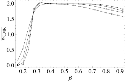
Figure 1: Average number of wrapping CMR clusters, $\overline{w_{\rm CMR}}$ vs.  $\beta$ for the 3D EA model.

Figure 2 shows the fraction of sites in the largest CMR blue cluster, ${\cal C}_{1}$, second largest CMR blue cluster, ${\cal C}_{2}$ and the sum of the two, ${\cal C}_{1}+{\cal C}_{2}$. The middle set of four curves is ${\cal C}_{1}$ for sizes $6^{3}$, $8^{3}$, $10^{3}$ and $12^{3}$, ordered from top to the bottom at $\beta=0.5$. The bottom set of curves is ${\cal C}_{2}$ with systems sizes ordered from smallest on bottom to largest on top at $\beta=0.5$. The difference between the fraction of sites in the two largest clusters, ${\cal C}_{1}-{\cal C}_{2}$ is approximately the spin glass order parameter. As the system size increases, this difference decreases below the transition suggesting that ${\cal C}_{1}={\cal C}_{2}$ for $\beta<\beta_{c}$ in the thermodynamic limit. On the other hand, the sum of the two largest clusters is quite constant independent of system size. Near the transition, approximately 96% of the sites are in the two largest clusters.

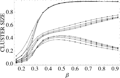
Figure 2: ${\cal C}_{1}$ (middle set), ${\cal C}_{2}$ (bottom set) and ${\cal C}_{1}+{\cal C}_{2}$ (top set) vs. $\beta$ for the CMR graphical representation for the 3D EA model.

The large fraction of sites in the two largest clusters makes the CMR cluster moves inefficient. If all sites were in the two largest clusters then the cluster moves would serve only to flip all spins in one or both clusters or exchange the identity of the two replicas. Equilibration depends on the small fraction of spins that are not part of the two largest clusters.

Figure 3 show the average number of wrapping TRFK clusters $\overline{w_{\rm TRFK}}$ as a function of inverse temperature. The largest system size is on the bottom for the small $\beta$ and on top for the large $\beta$. As for the case of CMR clusters, the data suggests a transition at some $\beta_{{\rm TRFK},p}$ from zero to two wrapping TRFK clusters. Although the number of TRFK wrapping clusters is significantly less than two for all $\beta$ and all system sizes, the trend in system size suggests that it might approach two for large systems and $\beta>\beta_{{\rm TRFK},p}$.

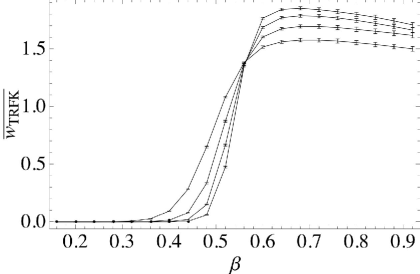
Figure 3: Average number of doubly occupied wrapping Fortuin-Kasteleyn clusters, $\overline{w_{\rm TRFK}}$ vs. $\beta$ for the 3D EA model.

The percolation signature for both CMR and TRFK clusters is qualitatively similar in three dimensions. In both cases two giant clusters with opposite values of the local order parameter appear at a temperature substantially above the phase transition temperature. In the high temperature phase, the two giant clusters have the same density and the phase transition is marked by the onset of different densities of the two clusters. The numerical evidence, however, suggests that the transition from equal to unequal giant cluster densities is quite broad for the small system sizes explored here.

V Discussion

We begin by noting that our results, even for the SK infinite-range spin glass, are not used to prove a phase transition (which has already been proved using other techniques ALR87 ). Rather, we use as an input the fact that such a transition exists and that the EA order parameter is zero above $T_{c}$ and nonzero below, and then show that the transition coincides exactly with the onset of a density difference in doubly occupied FK clusters. Numerical evidence indicates that something similar is occurring in the EA model. Together these complementary approaches shed light on the nature of the spin glass transition, especially from a geometric viewpoint, and suggest a possible framework through which a spin glass phase transition in realistic spin glass models can be finally proved.

We now summarize our results. We have introduced a random cluster approach for studying phase transitions and broken symmetry in spin glasses, both short- and infinite-range. We have shown that, unlike for ferromagnetic models, single FK percolation is a necessary but not sufficient condition for broken spin flip symmetry. However, double FK percolation (with a unique largest cluster) is sufficient and probably necessary. (More precisely, it is necessary in the SK model, because otherwise the EA order parameter is zero; and it is probably necessary in the EA model.)

In the SK model, there is a difference above $T_{c}$ between the CMR and TRFK approaches, but not below. In the former, there already is double percolation below $\beta_{c}$, above an onset inverse temperature of $\beta_{{\rm CMR},p}=N^{-1/2}$, below which there are no giant clusters. Between this inverse temperature and $\beta_{c}$ (which equals one in the class of models we study) there are exactly two giant clusters of equal density, which become $1/2$ in the $N\to\infty$ limit.

More importantly, there is a second transition occurring at exactly the SK spin glass critical value $\beta_{c}=1$. Above this threshold, the two giant clusters take on unequal densities, whose sum is one (i.e., every bond and spin belong to one of the two giant clusters). It could be the case at some even higher $\beta$ there is only a single giant cluster, but our methods so far are unable to determine whether this is the case.

For TRFK percolation there are no giant clusters above $\beta_{{\rm TRFK},p}=1$. For $\beta>1$ there are exactly two giant clusters with unequal densities, and the picture then becomes similar to that of the CMR representation.

The numerical simulations of the 3D EA model suggest a scenario similar to what we find in the SK model. We observe a sharp percolation transition for both the CMR and TRFK representations at a temperature well above the spin glass transition temperature. At this percolation transition, two giant clusters form with opposite values of the EA order parameter. These clusters are nearly equal in density and together occupy most of the system. As the temperature is decreased toward the presumed location of the spin glass transition, the density of the two clusters becomes increasingly unequal. Although this transition in the density of the two largest clusters appears quite rounded for the small systems investigated numerically, we believe it is sharp in the thermodynamic limit. The results for both the SK model and the connection between the EA order parameter and the density difference between giant clusters strongly suggests that the spin glass transition in finite dimensions is marked by the onset of this density difference in both the CMR and TRFK representations. These results provide an interesting geometric avenue for investigating the phase transition in the EA model and related models with frustration such as the random bond Ising model or the Potts spin glass.

- (1) K. Binder and A. P. Young. Spin glasses: experimental facts, theoretical concepts, and open questions. Rev. Mod. Phys., 58:801–976, 1986.
- (2) E. Marinari, G. Parisi, F. Ricci-Tersenghi, J. J. Ruiz-Lorenzo, and F. Zuliani. Replica symmetry breaking in spin glasses: Theoretical foundations and numerical evidences. J. Stat. Phys., 98:973–1047, 2000.
- (3) C. M. Newman and D. L. Stein. Topical Review: Ordering and broken symmetry in short-ranged spin glasses. J. Phys.: Cond. Mat., 15:R1319 – R1364, 2003.
- (4) D. Sherrington and S. Kirkpatrick. Solvable model of a spin glass. Phys. Rev. Lett., 35:1792–1796, 1975.
- (5) M. Aizenman, J. L. Lebowitz, and D. Ruelle. Some rigorous results on the Sherrington-Kirkpatrick spin glass model. Commun. Math. Phys., 112:3–20, 1987.
- (6) S. Edwards and P. W. Anderson. Theory of spin glasses. J. Phys. F, 5:965–974, 1975.
- (7) M. E. Fisher and R. R. P. Singh. Critical points, large-dimensionality expansions and Ising spin glasses. In G. Grimmett and D. J. A. Welsh, editors, Disorder in Physical Systems, pages 87–111. Clarendon Press, Oxford, 1990.
- (8) M. J. Thill and H. J. Hilhorst. Theory of the critical state of low-dimensional spin glass. J. Phys. I, 6:67–95, 1996.
- (9) G. Kotliar, P. W. Anderson, and D. L. Stein. A one-Dimensional spin glass model with long-range random interactions. Phys. Rev. B, 27:602–605, 1983.
- (10) A. T. Ogielski. Dynamics of three-dimensional spin glasses in thermal equilibrium. Phys. Rev. B, 32:7384–7398, 1985.
- (11) A. T. Ogielski and I. Morgenstern. Critical behavior of the three-dimensional Ising spin-glass model. Phys. Rev. Lett., 54:928–931, 1985.
- (12) N. Kawashima and A. P. Young. Phase transition in the three-dimensional Ising spin glass. Phys. Rev. B, 53:R484–R487, 1996.
- (13) E. Marinari, G. Parisi, and F. Ritort. On the Ising spin glass. J. Phys. A, 27:2687–2708, 1994.
- (14) P. W. Kasteleyn and C. M. Fortuin. Phase transitions in lattice systems with random local properties. J. Phys. Soc. Jpn. [Suppl.], 26:11–14, 1969.
- (15) C. M. Fortuin and P. W. Kasteleyn. On the random-cluster model. I. Introduction and relation to other models. Physica, 57:536–564, 1972.
- (16) M. Sweeny. Monte Carlo study of weighted percolation clusters relevant to the Potts model. Phys. Rev. B, 27:4445–4455, 1983.
- (17) R. H. Swendsen and J.-S. Wang. Replica Monte Carlo simulations of spin glasses. Phys. Rev. Lett., 57:2607–2609, 1986.
- (18) U. Wolff. Collective Monte Carlo updating for spin systems. Phys. Rev. Lett., 62:361–364, 1989.
- (19) M. Aizenman, J. T. Chayes, L. Chayes, and C. M. Newman. The phase boundary in dilute and random Ising and Potts ferromagnets. J. Phys. A Lett., 20:L313–L318, 1987.
- (20) J. Imbrie and C. M. Newman. An intermediate phase with slow decay of correlations in one dimensional percolation, Ising and Potts models. Commun. Math. Phys., 118:303–336, 1988.
- (21) J. Machta, C. M. Newman, and D. L. Stein. The percolation signature of the spin glass transition. J. Stat. Phys, 130:113–128, 2008.
- (22) J. Machta, C. M. Newman, and D. L. Stein. Percolation in the Sherrington-Kirkpatrick spin glass. In V. Sidoravicious and M. E. Vares, editors, Progress in Probability Vol. 60: In and Out of Equilibrium 2. Birkhäuser, Boston, arXiv:0710.1399.
- (23) L. Chayes, J. Machta, and O. Redner. Graphical representations for Ising systems in external fields. J. Stat. Phys., 93:17–32, 1998.
- (24) O. Redner, J. Machta, and L. F. Chayes. Graphical representations and cluster algorithms for critical points with fields. Phys. Rev. E, 58:2749–2752, 1998.
- (25) C. M. Newman and D. L. Stein. Short-range spin glasses: Results and speculations. In E. Bolthausen and A. Bovier, editors, Spin Glasses (Lecture Notes In Mathematics, v. 100), pages 159–175. Springer, Berlin, 2007.
- (26) J.-S. Wang and R. H. Swendsen. Low temperature properties of the J Ising spin glass in two dimensions. Phys. Rev. B, 38:4840–4844, 1988.
- (27) Y. Kasai and A. Okiji. Percolation problem describing ising spin glass system. Prog. Theor. Phys., 79:1080–1094, 1988.
- (28) C. M. Newman. Disordered Ising systems and random cluster representations. J. Phys.: Cond. Mat., 15:R1319 – R1364, 1992.
- (29) R. M. Burton and M. Keane. Density and uniqueness in percolation. Commun. Math. Phys., 121:501–505, 1989.
- (30) A. Gandolfi, M. Keane, and C. M. Newman. Uniqueness of the infinite component in a random graph with applications to percolation and spin glasses. Probab. Th. Rel. Fields, 92:511–527, 1992.
- (31) L. de Arcangelis, A. Coniglio, and F. Peruggi. Percolation transition in spin glasses. Europhysics Letters, 14:515–519, 1991.
- (32) H.-G. Katzgraber, M. Körner, and A. P. Young. Universality in three-dimensional Ising spin glasses: A Monte Carlo study. Phys. Rev. B, 73:224432–1–224432–11, 2006.
- (33) R. G. Edwards and A. D. Sokal. Generalizations of the Fortuin-Kasteleyn-Swendsen-Wang representation and Monte Carlo algorithm. Phys. Rev. D, 38:2009–2012, 1988.
- (34) B. Bollobás. Random Graphs, 2nd ed. Cambridge Univ. Press, Cambridge, 2001.
- (35) P. Erdös and E. Rényi. On the evolution of random graphs. Magyar Tud. Akad. Mat. Kutató Int. Közl, 5:17–61, 1960.
- (36) M. Mézard, G. Parisi, N. Sourlas, G. Toulouse, and M. Virasoro. Nature of the spin glass phase. Phys. Rev. Lett., 52:1156–1159, 1984.
- (37) J.-S. Wang and R. H. Swendsen. Replica Monte Carlo simulation (revisited). Prog. Theor. Phys. Suppl., 157:317–323, 2005.
- (38) J. Houdayer. A cluster Monte Carlo algorithm for 2-dimensional spin glasses. European Physical Journal B, 22:479–484, 2001.
- (39) T. Jörg. Cluster Monte Carlo algorithms for diluted spin glasses. Prog. Theor. Phys. Suppl., 157:349–352, 2005.
- (40) T. Jörg. Critical behavior of the three-dimensional bond-diluted Ising spin glass: Finite-size scaling functions and universality. Phys. Rev. B, 73:224431–1–22443–9, 2006.