INSTITUT NATIONAL DE RECHERCHE EN INFORMATIQUE ET EN AUTOMATIQUE

Bounds for self-stabilization in unidirectional networks
Samuel Bernard^⋆ — Stéphane Devismes^∘ — Maria Gradinariu Potop-Butucaru^⋆,† — Sébastien Tixeuil^{⋆,‡ ⋆} Université Pierre et Marie Curie - Paris 6, LIP6, France
^∘ CNRS, LRI, France
^† INRIA project-team Regal
^‡ INRIA project-team Grand Large N° 6524
May 2008

Abstract: A distributed algorithm is self-stabilizing if after faults and attacks hit the system and place it in some arbitrary global state, the systems recovers from this catastrophic situation without external intervention in finite time. Unidirectional networks preclude many common techniques in self-stabilization from being used, such as preserving local predicates. In this paper, we investigate the intrinsic complexity of achieving self-stabilization in unidirectional networks, and focus on the classical vertex coloring problem.

When deterministic solutions are considered, we prove a lower bound of $n$ states per process (where $n$ is the network size) and a recovery time of at least $n(n-1)/2$ actions in total. We present a deterministic algorithm with matching upper bounds that performs in arbitrary graphs. When probabilistic solutions are considered, we observe that at least $\Delta+1$ states per process and a recovery time of $\Omega(n)$ actions in total are required (where $\Delta$ denotes the maximal degree of the underlying simple undirected graph). We present a probabilistically self-stabilizing algorithm that uses $\mathtt{k}$ states per process, where $\mathtt{k}$ is a parameter of the algorithm. When $\mathtt{k}=\Delta+1$, the algorithm recovers in expected $O(\Delta n)$ actions. When $\mathtt{k}$ may grow arbitrarily, the algorithm recovers in expected $O(n)$ actions in total. Thus, our algorithm can be made optimal with respect to space or time complexity.

Key-words: self-stabilization, lower bounds, unidirectional networks, coloring

Bornes pour l’auto-stabilisation dans les réseaux unidirectionnels

Résumé : Un algorithme réparti est auto-stabilisant si, après que des fautes et des attaques aient frappé le système et l’aient placé dans un état quelconque, le système corrige cette situation catastrophique sans intervention extérieure en temps fini. Les réseaux unidirectionels empêchent de nombreuses techniques habituelles dans le cadre de l’auto-stabilisation d’être utilisées, comme la préservation de prédicats locaux. Dans cet article, nous évaluons la complexité intrinsèque de la réalisation de l’auto-stabilisation dans les réseaux unidirectionels, et nous nous concentrons sur le problème du coloriage de nœuds.

Quand les solutions déterministes sont envisagées, nous prouvons qu’il existe une borne inférieure de $n$ états par processus (où $n$ est la taille du réseau) et un temps minimal avant retour à la normale de $n(n-1)/2$ action au total. Nous présentons un algorithme déterministe dans des réseaux de topologies quelconques qui est optimal en espace et en temps.

Dans le cadre de solutions probabilistes, nous observons que $\Delta+1$ états par processus et $\Omega(n)$ actions au total sont requises (où $\Delta$ représente le degré du graphe non-orienté sous-jacent). Nous présentons un algorithme auto-stabilisant probabiliste qui utilise $\mathtt{k}$ états par processus, où $\mathtt{k}$ est un paramètre de l’algorithme. Quand $\mathtt{k}=\Delta+1$, l’algorithme retrouve un comportement correct en $O(\Delta n)$ actions en moyenne. Mais si $\mathtt{k}$ augmente de manière arbitraire, l’algorithme retrouve un comportement correct en $O(n)$ actions en moyenne. Au final, notre algorithme peut être rendu optimal en espace ou en temps.

Mots-clés : auto-stabilisation, bornes inférieures, réseaux unidirectionels, coloriage

1 Introduction

One of the most versatile technique to ensure forward recovery of distributed systems is that of self-stabilization [9, 10]. A distributed algorithm is self-stabilizing if after faults and attacks hit the system and place it in some arbitrary global state, the systems recovers from this catastrophic situation without external (e.g. human) intervention in finite time. Self-stabilization makes no hypotheses about the extent or the nature of the faults and attacks that may harm the system, yet may induce some overhead (e.g. memory, time) when there are no faults, compared to a classical (i.e. non-stabilizing) solution. Computing space and time bounds for particular problems in a self-stabilizing setting is thus crucial to evaluate the impact of adding forward recovery properties to the system.

The vast majority of self-stabilizing solutions in the literature [10] considers bidirectional communications capabilities, i.e. if a process $u$ is able to send information to another process $v$, then $v$ is always able to send information back to $u$. This assumption is valid in many cases, but can not capture the fact that asymmetric situations may occur, e.g. in wireless networks, it is possible that $u$ is able to send information to $v$ yet $v$ can not send any information back to $u$ ($u$ may have a wider range antenna than $v$). Asymmetric situations, that we denote in the following under the term of unidirectional networks, preclude many common techniques in self-stabilization from being used, such as preserving local predicates (a process $u$ may take an action that violates a predicate involving its outgoing neighbors without $u$ knowing it, since $u$ can not get any input from them).

Related works

Self-stabilization in bidirectional networks makes a distinction between global tasks (i.e. tasks whose specification forbids particular state combinations of processes arbitrarily far from one another in the network, such as leader election) and local tasks (whose specifications forbid particular state combinations only for processes that are at distance at most $d$ from one another, for some parameter $d$). Local tasks are often considered easier in bidirectional networks since detecting incorrect situations requires less memory and computing power [3], recovering can be done locally [2], and Byzantine containment can be guaranteed [19, 21].

Since a self-stabilizing algorithm may start from any arbitrary state, lower bounds for non-stabilizing (a.k.a. properly initialized) distributed algorithms still hold for self-stabilizing ones. As a result, relatively few works investigate lower bounds that are specific to self-stabilization [4, 11, 12, 14, 17, 22]. Results related to space lower bounds deal with global tasks (e.g. constructing a spanning tree [11], finding a center [11], electing a leader [4, 11], passing a token [12, 14, 22], etc.). [17] provides a time lower bound for self-stabilizing token passing, still a global task. Global tasks typically require $\Omega(n)$ states per process (i.e. $\Omega(\log(n)$ bits per process) and $\Omega(n)$ time complexity to recover from faults.

Investigating the possibility of self-stabilization in unidirectional networks was recently emphasized in several papers [1, 5, 6, 8, 13, 15, 16]. In particular, [6] show that in the simple case of acyclic unidirectional networks, nearly any recursive function can be computed anonymously in a self-stabilizing way. Computing global tasks in a general topology requires either unique identifiers [1, 5, 13] or distinguished processes [8, 15, 16]. Observe that all aforementioned works consider global tasks, and provide constructive upper bound results (i.e algorithms), leaving the question of matching lower bounds open.

Our contribution

In this paper, we investigate the intrinsic complexity of achieving self-stabilization in unidirectional networks, and focus on the classical vertex coloring problem, a local task with several known efficient self-stabilizing solutions in bidirectional networks [18, 20]. Deterministic and probabilistic solutions require only a number of states that is proportional to the network maximum degree $\Delta$, and the number of actions per process in order to recover is $O(\Delta)$ (in the case of a deterministic algorithm) or expected $O(1)$ (in the case of a probabilistic one). To satisfy the vertex coloring specification in unidirectional networks, an algorithm must ensure that no two neighboring nodes (i.e. two nodes $u$ and $v$ such that either $u$ can send information to $v$, or $v$ can send information to $u$, but not necessarily both) have identical colors.

The main result of this paper is to show that solving a local task in unidirectional networks with a deterministic algorithm is as difficult as solving a global task in bidirectional networks, while nice complexity guarantees can be preserved with probabilistic solutions:

1. When deterministic solutions are considered, we prove a lower bound of $n$ states per process (where $n$ is the network size) and a recovery time of at least $n(n-1)/2$ actions in total. We present a deterministic algorithm with matching upper bounds that performs in arbitrary graphs.

2. When probabilistic solutions are considered, we observe that at least $\Delta+1$ states per process and a recovery time of $\Omega(n)$ actions in total are required. We present a probabilistically self-stabilizing algorithm that uses $\mathtt{k}$ states per process, where $\mathtt{k}$ is a parameter of the algorithm. When $k=\Delta+1$, the algorithm recovers in expected $O(\Delta n)$ actions. When $\mathtt{k}$ may grow arbitrarily, the algorithm recovers in expected $O(n)$ actions in total. Thus, our algorithm can be made optimal with respect to space or time complexity.

Outline

The remaining of the paper is organized as follows: Section 2 presents the programming model and problem specification, Section 3 provides impossibility results and lower bounds for our problem, while Sections 4 and 5 present matching upper bounds (in the deterministic case) and asymptotically matching upper bounds (in the probabilistic case). Section 6 gives some concluding remarks and open questions.

2 Model

Program model

A program consists of a set $V$ of $n$ processes. A process maintains a set of variables that it can read or update, that define its state. Each variable ranges over a fixed domain of values. We use small case letters to denote singleton variables, and capital ones to denote sets. A process contains a set of constants that it can read but not update. A binary relation $E$ is defined over distinct processes such that $(i,j)\in E$ if and only if $j$ can read the variables maintained by $i$; $i$ is a predecessor of $j$, and $j$ is a successor of $i$. The set of predecessors (resp. successors) of $i$ is denoted by $P.i$ (resp. $S.i$), and the union of predecessors and successors of $i$ is denoted by $N.i$, the neighbors of $i$. In some case, we are interested in the iterated notions of those sets, e.g. $S.i^{0}={i}$, $S.i^{1}=S.i$, …, $S.i^{k}=\cup_{j\in S.i}S.j^{k-1}$. The values $\delta_{in}.i$, $\delta_{out}.i$, and $\delta.i$ denote respectively $|P.i|$, $|S.i|$, and $|N.i|$; $\Delta_{in}$, $\Delta_{out}$, and $\Delta$ denote the maximum possible values of $\delta_{in}.i$, $\delta_{out}.i$, and $\delta.i$ over all processes in $V$.

An action has the form $\langle name\rangle:\langle guard\rangle\longrightarrow\langle command\rangle$. A guard is a Boolean predicate over the variables of the process and its communication neighbors. A command is a sequence of statements assigning new values to the variables of the process. We refer to a variable $v$ and an action $a$ of process $i$ as $v.i$ and $a.i$ respectively. A parameter is used to define a set of actions as one parameterized action.

A configuration of the program is the assignment of a value to every variable of each process from its corresponding domain. Each process contains a set of actions. An action is enabled in some configuration if its guard is true in this configuration. A computation is a maximal sequence of configurations such that for each configuration $\gamma_{i}$, the next configuration $\gamma_{i+1}$ is obtained by executing the command of at least one action that is enabled in $\gamma_{i}$. Maximality of a computation means that the computation is infinite or it terminates in a configuration where none of the actions are enabled. A program that only has terminating computations is silent.

A scheduler is a predicate on computations, that is, a scheduler is a set of possible computations, such that every computation in this set satisfies the scheduler predicate. We distinguish two particular schedulers in the sequel of the paper: the distributed scheduler corresponds to predicate true (that is, all computations are allowed); in contrast, the locally central scheduler implies that in any configuration belonging to a computation satisfying the scheduler, no two enabled actions are executed simultaneously on neighboring processes.

A configuration conforms to a predicate if this predicate is true in this configuration; otherwise the configuration violates the predicate. By this definition every configuration conforms to predicate true and none conforms to false. Let $R$ and $S$ be predicates over the configurations of the program. Predicate $R$ is closed with respect to the program actions if every configuration of the computation that starts in a configuration conforming to $R$ also conforms to $R$. Predicate $R$ converges to $S$ if $R$ and $S$ are closed and any computation starting from a configuration conforming to $R$ contains a configuration conforming to $S$. The program deterministically stabilizes to $R$ if and only if true converges to $R$. The program probabilistically stabilizes to $R$ if and only if true converges to $R$ with probability $1$.

Problem specification

Consider a set of colors ranging from $0$ to $\mathtt{k}-1$, for some integer $\mathtt{k}\geq 1$. Each process $i$ defines a function $\mathit{color}.i$ that takes as input the states of $i$ and its predecessors, and outputs a value in $\{0,\ldots,\mathtt{k}-1\}$. The unidirectional vertex coloring predicate is satisfied if and only if for every $(i,j)\in E$, $\mathit{color}.i\neq\mathit{color}.j$.

3 Impossibility results and lower bounds

General bounds

We first observe two lower bounds that hold for any kind of silent program that is self-stabilizing or probabilistically self-stabilizing for the unidirectional coloring specification:

1. The minimal number of states per process is $\Delta+1$. Consider a bidirectional clique network (that is $(\Delta+1)$-sized), and a terminal configuration of the program. Suppose that only $\Delta$ states are used, then at least two processes $i$ and $j$ have the same state, and have the same view of their predecessors. As a result $\mathit{color}.i=\mathit{color}.j$, and $i$ and $j$ being neighbors, the unidirectional coloring predicate does not hold in this terminal configuration.

2. The minimal number of moves overall is $\Omega(n)$. Consider a unidirectional chain of processes which are all initially in the same state. For every process but one, the color is identical to that of its predecessor. Since a change of state may only resolve two conflicts (that of the moving node and that of its successor), a number of overall moves at least equal to $\lfloor n/2\rfloor$ is required, thus $\Omega(n)$ moves.

Deterministic bounds

The rest of the section is dedicated to deterministic impossibility results and lower bounds. Theorem 1 (presented below) shows that if unconstrained schedules (i.e. the scheduler is distributed) are allowed, some initial symmetric configurations can not be broken afterwards, making the unidirectional coloring problem impossible to solve by a deterministic algorithm. This justifies the later assumption of a locally central scheduler in Section 4, i.e. a scheduler that never schedules for execution two neighboring activatable processes simultaneously.

Lemma 1

Let an unidirectional network $\{p_{0},p_{1},\ldots,p_{n-1}\}$ of size $n$. Consider every node executes a uniform deterministic self-stabilizing uniform coloring algorithm. Whenever there exists $i$ such that $s.p_{i}=s.p_{(i-1)\bmod n}$, $p_{i}$ is activatable and if activated would change its state to $s^{\prime}.p_{i}$ with $s^{\prime}.p_{i}\neq s.p_{i}$.

Proof.

We first show that $p_{i}$ is activatable. Assume the contrary, and consider a uniform cycle of $n$ nodes that are all in the same state. If $p_{i}$ is not activatable, none of the remaining processes is activatable either. Hence, the configuration is terminal. Now, a process $p_{i}$ may only read its own state and that of its predecessor in the cycle, so the color $\mathit{color}.p_{i}$ is uniquely determined by these two values only. Moreover, the $\mathit{color}.p_{i}$ is the same as $\mathit{color}.p_{(i-1)\bmod n}$. So, the configuration is terminal and two neighboring processes have the same color. This contradicts the fact that the algorithm is a deterministic self-stabilizing unidirectional coloring one.

Then we show that $p_{i}$, if activated moves to a different state $s^{\prime}.p_{i}$. Assume $p_{i}$ moves to the same state $s.p_{i}$, then if the starting configuration is such that all nodes have the same state, then no node is able to change its state, the algorithm being uniform. Since this configuration can not be a coloring, the system never changes the global configuration and thus is not self-stabilizing. ∎

Theorem 1

There exists no uniform deterministic self-stabilizing coloring algorithm that can run on any unidirectional graph under a distributed scheduler.

(a) uniform configuration in state $s$

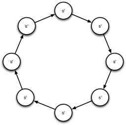
(b) uniform configuration in state $s^{\prime}$

Figure 1: A possible execution with synchronous scheduling

Proof.

Assume the contrary. Consider a unidirectional cycle $\{p_{0},p_{1},\ldots,p_{n-1}\}$ of size $n$. Assume that in the initial state all nodes are in the same state $s$ (see Figure 1.(a)). By Lemma 1, all nodes are activatable, and if a node is activated by the scheduler, it moves to a different state $s^{\prime}$. Consider the synchronous scheduler that, at each step, activates all nodes. Then, after one scheduler activation, all nodes have state $s^{\prime}$ (see Figure 1.(b)). After another activation, all nodes move to state $s^{\prime\prime}$, etc. In this infinite execution, every configuration has all nodes with the same state and thus, the coloration problem is not solved. As a result, the algorithm can not be self-stabilizing. ∎

Notice that the result of Theorem 1 holds even if the program is not required to be silent or if participating processes have infinite number of states.

From now on, we assume the scheduler is locally central. We demonstrate that a uniform silent deterministic self-stabilizing algorithm for the unidirectional coloring problem must use at least $n$ states per process in general networks. The proof is by exhibiting a particular family of networks (namely, $n$-sized cycles) in which the bound is reached by any such algorithm even assuming a locally central scheduler.

process $i$
const
	k : integer
	$p.i$ : predecessor of $i$
var
	$c.i$ : color of node $i$
action
	$c.i=c.p.i$ $\rightarrow$
		$c.i:=c.i+1\mathrm{mod}\mathtt{k}$

Algorithm 1 A uniform deterministic coloring algorithm for unidirectional rings

Lemma 2

Consider a unidirectional cycle $\{p_{0},p_{1},\ldots,p_{n-1}\}$ of size $n$. Consider a scheduler that only activates a node $p_{i}$ when $s.p_{i}=s.p_{(i-1)\bmod n}$. Assume every node executes a uniform deterministic self-stabilizing unidirectional coloring algorithm that uses a finite number of states $K$. There exists an initial configuration such that the state sequence starting from this configuration is isomorphic to that of Algorithm 1, for some parameter $k\leq K$.

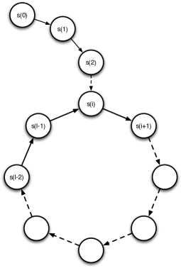
(a) state transition function of a uniform deterministic self-stabilizing algorithm

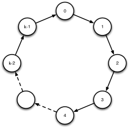
(b) state transition function of Algorithm 1

Figure 2: Isomorphism of the state transition function when $s.p_{i}=s.p_{i-1\bmod n}$

Proof.

Consider a unidirectional cycle $\{p_{0},p_{1},\ldots,p_{n-1}\}$ of size $n$. Assume a node $p_{i}$ is activated only when its state $s.p_{i}$ is equal to $s.p_{(i-1)\bmod n}$, the state of the predecessor of $p_{i}$ in the cycle. Then, the transition function of node $p_{i}$ is solely based on the state $s.p_{i}$. Let $s(0),s(1),\ldots$ the sequence of states returned by the transition function of process $p_{i}$ executing the self-stabilizing coloring algorithm started in an arbitrary state $s(0)$. Note that (i) the number of states is finite, (ii) a process with the same state as its predecessor is always activatable (Lemma 1), and (iii) the protocol is deterministic. Then, the shape of the transition function of $p_{i}$ is as depicted in Figure 2.(a). That is, there exist $i$ and $l$ ($i<l$) such that $s(i)=s(l)$ and $l-i\leq K$. Since the protocol is self-stabilizing, it may be started from any arbitrary state, and in particular from state $s(i)$ (in Figure 2.(a)). Let denote $s(j)$ by $j-i$, $\forall i\leq j<l$. The transition function of $p_{i}$ is isomorphic to that of the same process executing Algorithm 1 (given in Figure 2(b)) and assuming $k=l-i$. ∎

Theorem 2

A silent uniform deterministic self-stabilizing protocol for unidirectional coloring requires at least $n$ states per process in a $n$-sized network (with $n\geq 2$).

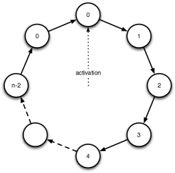
(a) starting configuration

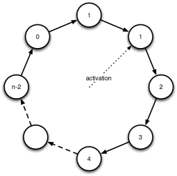
(b) after $1$ step

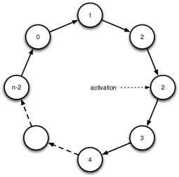
(c) after $2$ steps

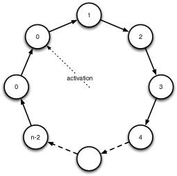
(d) after $n-1$ steps

Figure 3: A possible execution of Algorithm 1

Proof.

Assume there exists a silent uniform deterministic self-stabilizing protocol for coloring that requires less than $n$ states for a particular node. Since the protocol is uniform, every node must use $k<n$ states.

Consider a unidirectional cycle $\{p_{0},p_{1},\ldots,p_{n-1}\}$ of size $n$. In what follows, we consider executions of the protocol in which the scheduler only activates nodes that have the same state as their predecessor. By Lemma 2, the transition function of every node is isomorphic to that of Algorithm 1, so we assume all nodes execute Algorithm 1 with $k<n$.

In the following, we consider $k=n-1$ but the proof is easily expendable to any $k<n$ by putting the $n-k+1$ last processors in the same state. Now consider the unidirectional ring presented in Figure 3.(a). The scheduler only activates the single node with the same state $0$ as its parent, and reach the configuration presented in Figure 3.(b). The scheduler may now activate the single node with the same state $1$ as its parent and reach the configuration presented in Figure 3.(c). We repeat the argument and reach the configuration presented in Figure 3.(d). This configuration is symmetric to that of the configuration presented in Figure 3.(a), so the process can repeat infinitely often. As a result, the protocol is not silent. ∎

We now address the question of time lower bounds for deterministic self-stabilizing programs for the unidirectional coloring problem.

Theorem 3

A silent uniform deterministic self-stabilizing protocol for unidirectional coloring converges in at least $\frac{n(n-1)}{2}$ steps in general graphs.

Proof.

Consider a chain topology, and assume that processors are ordered from the sink $p_{1}$ to the source $p_{n}$. Assume all processors are initially in the same state (a self-stabilizing program may start from any arbitrary configuration). We now consider a locally central scheduler that activates nodes according to the schedule presented in Schedule 1.

var
	$i$,$j$: integer
scheduler
	for $j$ from $n-1$ to $1$
		for $i$ from $1$ to $j$
			activate $p_{i}$

Schedule 1 Our $\frac{n(n-1)}{2}$-steps scheduling in $n$-sized chains

Schedule 1 selects a single process at a time for execution, thus it satisfies the locally central scheduler property. In addition, it only selects for execution a process that has the same state as its predecessor (and thus activatable by Lemma 1): if $p_{1}$ to $p_{k}$ have the same state $s$ then $p_{1}$ to $p_{k-1}$ are activatable and if they are activated in ascending order, $p_{1}$ to $p_{k-1}$ will move to the same “next” state $s^{\prime}$ (see Figure 2.(a)). So every process activation leads to an effective move and the total number of activations is $\sum_{i=1}^{n-1}i=\frac{n(n-1)}{2}$.

Finally, all executions of the protocol must be terminating (it is silent), and from an initial configuration where all processes have the same state, a locally central schedule (like Schedule 1) may leads to $n(n-1)/2$ steps at least before termination. Hence the result. ∎

4 Self-stabilizing deterministic unidirectional coloring

In this section we propose a time and space optimal silent self-stabilizing deterministic algorithm for unidirectional coloring. The algorithm is referred thereafter as Algorithm 2 and performs under the locally central scheduler. The algorithm can be informally described as follows: each process $i$ has an integer variable $c.i$ (that ranges from $0$ to $\mathtt{k}-1$, where $\mathtt{k}$ is a parameter of the algorithm) that denotes its color; whenever a node has the same color as one of its predecessors, it changes its color to the next available color (using the classical total order on integers). Here, the $\mathit{color}.i$ function simply returns the color variable $c.i$ of $i$.

process $i$
const
	k : integer
	$P.i$ : set of predecessors of $i$
parameter
	$p$ : node in $P.i$
var
	$c.i$ : color of node $i$
action
	$p\in P.i$, $c.i=c.p$ $\rightarrow$
		do $p\in P.i$, $c.i=c.p$ $\rightarrow$
			$c.i:=c.i+1\mathrm{mod}\mathtt{k}$
		od

Algorithm 2 A uniform deterministic coloring algorithm for general unidirectional networks

A configuration is legitimate if, for every process $i$, and for every predecessor $p\in P.i$, $c.i\neq c.p.i$. Obviously, a legitimate configuration satisfies the unidirectional coloring predicate (assuming $\mathit{color}.i$ return $c.i$) and is terminal (all guarded commands are disabled). There remains to show how fast the algorithm attains a legitimate configuration in the worst case for every possible locally central schedule.

Theorem 4

Algorithm 2 is a (state-optimal) uniform silent deterministic self-stabilizing protocol for coloring nodes in unidirectional general networks of size $n$ (when $\mathtt{k}=n$), assuming a locally central scheduler and converges in $\frac{n(n-1)}{2}$ steps to a legitimate configuration.

Proof.

Assume Algorithm 2 starts in an arbitrary initial configuration $c$. We now consider the table that lists, for every possible color (in the set $\{0,\ldots,n-1\}$ since we assume $\mathtt{k}=n$), the processes that currently have this color. An example of such a table is presented as Table 1, where processes $P_{3}$ and $P_{2}$ have color $0$, process $P_{n-2}$ has color $n-1$, etc. This table is denoted in the sequel as the color table.

Processors	$P_{3},P_{2}$		$P_{n-1},P_{1}$		…	$P_{n-2}$
States	$0$	$1$	$2$	$3$	…	$n-1$

Table 1: An example of color table

According to Algorithm 2 the evolution of the color table follows two rules:

1. A cell containing one process can not become empty. That is, a process having a color not used by any other process in the system can not be activated. In our algorithm, this is due to the fact that processes are activatable only if they share their color with their predecessor.

2. A process only moves to the right (in a cyclic manner) and can not jump over an empty cell. Indeed, when activated, a process chooses the first “next” (in the sense of the usual total order on integers) unconflictual color hence the processes always move to the right. A process may move by several positions, but never skips a free position (this would mean that a process does not choose the ”next” color although this color is not conflicting with any other process and thus not with the process predecessors).

Since there are $n$ cells and $n$ processes, every process could be placed in a different cell if necessary. Since a process can not jump over an empty cell, after $n-1$ moves, a process is sure to find a free cell. In fact, the number of moves a process may have to perform to reach a free cell depends on the number of free cells. With $k$ free cells, there are at most $n-k$ consecutive non-empty cells that could potentially provoke further conflicts. A process, in order to reach a free cell has to perform at most $n-k$ moves. Once this process occupies a free cell, the number of free cells decreases to $k-1$. Starting with $n-1$ free cell (every process has the same color), and finishing with $1$, at most $1+2+...+(n-1)=\frac{n(n-1)}{2}$ steps are needed to have every process in a free cell or with a non-conflicting color (i.e. different from that of its predecessors) and thus reach a legitimate configuration. ∎

5 Probabilistic self-stabilizing unidirectional coloring

In Section 3, we observed that there exist lowers bounds even for probabilistic approaches to the unidirectional coloring problem. The space lower bound is $\Delta+1$ and the time lower bound is $n$ (where $\Delta$ and $n$ are the degree and the size of the underlying simple undirected graph, respectively).

The algorithm presented as Algorithm 3 can be informally described as follows. If a process has the same color as one of its predecessors then it chooses a new color in the set of available colors (i.e. the set of colors that are not already used by any of its predecessors). The colors are chosen in a set of size $\mathtt{k}$, where $\mathtt{k}$ is a parameter of the algorithm. In the following, we show that Algorithm 3 is probabilistically self-stabilizing for the unidirectional coloring problem if $\mathtt{k}>\Delta$. To reach that goal we proceed in two steps: first we show that any terminal configuration satisfies the unidirectional coloring predicate (Lemma 3); secondly, we show that the expected number of steps to reach a terminal configuration starting from an arbitrary one is bounded (Lemma 7).

process $i$
const
	k : integer
	$P.i$ : set of predecessors of $i$
	$C.i$ : set of colors of nodes in $P.i$
parameter
	$p$ : node in $P.i$
var
	$c.i$ : color of node $i$
action
	$p\in P.i$, $c.i=c.p$ $\rightarrow$
		$c.i:=\mathtt{random}\left(\{0,\ldots,\mathtt{k}-1\}\setminus C.i\right)$

Algorithm 3 A uniform probabilistic coloring algorithm for general unidirectional networks

Lemma 3

Any terminal configuration satisfies the unidirectional coloring predicate.

Proof.

In a terminal configuration, every process $i$ satisfies $\forall j\in P.i,c.i\neq c.j$ and $\forall j\in S.i,c.i\neq c.j$. Hence, in a terminal configuration, every process $i$ has a color that is different from those of its neighbors, which proves the theorem. ∎

Definition 1 (Conflict)

Let $p$ be a process and $\gamma$ a configuration. The tuple $(p$,$\gamma)$ is called a conflict if and only if there exists $q\in P.p$ (the predecessors of $p$) such that $c.q=c.p$ in $\gamma$.

Lemma 4

Assume $\mathtt{k}>\Delta$. Let $(p$,$\gamma)$ be a conflict. The expected number of conflicts created by the execution of one step of $p$ in order to resolve $(p$,$\gamma)$ is:

$$\frac{\delta.p-\delta_{in}.p}{\mathtt{k}-\delta_{in}.p}$$ (1)

Proof.

When a process $p$ executes Action $\mathtt{A}$ from $\gamma$, it chooses a new color in a set of at least $\mathtt{k}-\delta_{in}.p$ colors. That is, there are $\mathtt{k}$ colors and it can not choose a color chosen by one of its predecessors, therefore at most $\delta_{in}.p$ colors are removed from the set of possible choices.

For each $q\in S.p\wedge q\notin P.p$, $p$ and $q$ are in conflict if and only if, $p$ chooses the color of $q$. Notice that $p$ has $\frac{1}{(\mathtt{k}-\delta_{in}.p)}$ chance to create a new conflict. Since the number of successors of $p$ not in the set of predecessors of $p$, $\sharp\{q\in S.p\wedge q\notin P.p\}$, is $\delta.p-\delta_{in}.p$, the expected number of created conflicts is $\frac{\delta.p-\delta_{in}.p}{\mathtt{k}-\delta_{in}.p}$. ∎

Lemma 5

Let $(p,\gamma)$ be a conflict. The expected number of conflicts created by the execution of one step of $p$ in order to resolve $(p$,$\gamma)$ is less than or equal to:

$$\mathtt{M}=\frac{\Delta-1}{\mathtt{k}-1},~{}\mathtt{k}>\Delta$$ (2)

Proof.

Observe that $\forall p\in V,\Delta\geq\delta.p$, therefore $\forall p\in V,\frac{\delta.p-\delta_{in}.p}{\mathtt{k}-\delta_{in}.p}\leq\frac{\Delta-\delta_{in}.p}{\mathtt{k}-\delta_{in}.p}$. In order to find an upper bound for this value, let $f:p\in V,\Delta<\mathtt{k},\delta_{in}.p\in[0,\Delta],\delta_{in}.p\mapsto\frac{\Delta-\delta_{in}.p}{\mathtt{k}-\delta_{in}.p}$. Its derivative exists and is $f^{\prime}(\delta_{in}.p)=\frac{\Delta-\mathtt{k}}{(\mathtt{k}-\delta_{in}.p)^{2}}$. By hypothesis, $\mathtt{k}>\Delta$, so $f^{\prime}(\delta_{in}.p)<0$ and $f$ is decreasing. Therefore, $f(\delta_{in}.p)$ is maximum when $\delta_{in}.p=0$ but for this value $(p$,$\gamma)$ can not be a conflict. Therefore, $\delta_{in}.p\geq 1$ and $f$ is maximum for $\delta_{in}.p=1$ which leads to $\frac{\delta.p-\delta_{in}.p}{\mathtt{k}-\delta_{in}.p}\leq\frac{\Delta-\delta_{in}.p}{\mathtt{k}-\delta_{in}.p}\leq\frac{\Delta-1}{\mathtt{k}-1}$. ∎

Lemma 6

Let $(p,\gamma)$ be a conflict. The expected number of step created in order to resolve this conflict is less than:

$$\frac{\mathtt{k}-1}{\mathtt{k}-\Delta},~{}\mathtt{k}>\Delta$$ (3)

Proof.

From Lemma 5, the expected number of conflicts created by one step of $p$ is less than $\mathtt{M}=\frac{\Delta-1}{\mathtt{k}-1}$. Then, the processes in $S.p$ who received the created conflicts produce at most $\mathtt{M}$ new conflicts each since there are at most $\mathtt{M}$ expected such processes. They will perform $\mathtt{M}$ steps and create at most $\mathtt{M}^{2}=\left(\frac{\Delta-1}{\mathtt{k}-1}\right)^{2}$ new conflicts. Then the $\mathtt{M}^{2}$ processes in $S.p^{2}$ (the successors at distance two from $p$), after $\mathtt{M}^{2}$ step (one for each) will produce $\mathtt{M}^{3}$ new conflicts. By recurrence, at most $\mathtt{M}^{i}$ expected steps will be executed and $\mathtt{M}^{i+1}$ new conflicts will be created by the processes in $S.p^{i}$ (the successors at distance $i$ from $p$).

Finally, the expected number of steps executed is $\sum^{\infty}_{i=0}{\mathtt{M}^{i}}=\sum^{\infty}_{i=0}{\left(\frac{\Delta-1}{\mathtt{k}-1}\right)^{i}}$. Note that $\Delta\geq 1$ and $\mathtt{k}>\Delta$, so $0<\frac{\Delta-1}{\mathtt{k}-1}<1$. The expected number of steps executed in order to solve the conflict $(p,\gamma)$ is $\sum^{\infty}_{i=0}{\left(\frac{\Delta-1}{\mathtt{k}-1}\right)^{i}}=\frac{1}{1-\frac{\Delta-1}{\mathtt{k}-1}}=\frac{\mathtt{k}-1}{\mathtt{k}-\Delta}$ ∎

Lemma 7

Starting from an arbitrary configuration, the expected number of steps to reach a configuration verifying the unidirectional coloring predicate is less or equal to:

$$\frac{n(\mathtt{k}-1)}{\mathtt{k}-\Delta},~{}\mathtt{k}>\Delta$$ (4)

Proof.

In the worst case the number of initial conflicts is $n$. Then the proof is a direct consequence of Lemma 6. ∎

Notice that with a minimal number of colors (i.e., $\mathtt{k}=\Delta+1$), the expected number of steps to reach a terminal configuration starting from an arbitrary configuration is less than $n\Delta$. Moreover, when the number of colors increases (i.e., $\mathtt{k}\rightarrow\infty$), the expected number of steps to reach a terminal configuration starting from an arbitrary configuration converges to $n$.

Theorem 5

Algorithm 3 is a probabilistic self-stabilizing solution for the unidirectional coloring when $\mathtt{k}>\Delta$.

Proof.

The proof is a direct consequence of Lemma 3 and Lemma 7. ∎

6 Conclusion

We investigated the intrinsic complexity of performing local tasks in unidirectional networks in a self-stabilizing setting. Contrary to “classical” bidirectional networks, local vertex coloring now induces global complexity ($n$ states per process at least, $n$ moves per process at least) for deterministic solutions. We presented state and time optimal solutions for the deterministic case, and asymptotically optimal solutions for the probabilistic case. This work raises several important open questions:

1. Our probabilistic solution can be tuned to be optimal in space (and is then with a $\Delta$ multiplicative penalty in time), or optimal in time, but not both. However, our lower bounds do not preclude the existence of probabilistic solutions that are optimal for both complexity measures.

2. Several of the lower bounds we provide in the deterministic case rely on the silence property of the expected solution. We question the possibility of designing deterministic algorithms that are not silent yet provide coloring with less than $n$ colors in general graphs.

References

- [1] Yehuda Afek and Anat Bremler-Barr. Self-stabilizing unidirectional network algorithms by power supply. Chicago J. Theor. Comput. Sci., 1998, 1998.
- [2] Yehuda Afek and Shlomi Dolev. Local stabilizer. J. Parallel Distrib. Comput., 62(5):745–765, 2002.
- [3] Joffroy Beauquier, Sylvie Delaët, Shlomi Dolev, and Sébastien Tixeuil. Transient fault detectors. Distributed Computing, 20(1):39–51, 2007.
- [4] Joffroy Beauquier, Maria Gradinariu, and Colette Johnen. Randomized self-stabilizing and space optimal leader election under arbitrary scheduler on rings. Distributed Computing, 20(1):75–93, 2007.
- [5] Jorge Arturo Cobb and Mohamed G. Gouda. Stabilization of routing in directed networks. In Datta and Herman [7], pages 51–66.
- [6] Sajal K. Das, Ajoy Kumar Datta, and Sébastien Tixeuil. Self-stabilizing algorithms in dag structured networks. Parallel Processing Letters, 9(4):563–574, December 1999.
- [7] Ajoy Kumar Datta and Ted Herman, editors. Self-Stabilizing Systems, 5th International Workshop, WSS 2001, Lisbon, Portugal, October 1-2, 2001, Proceedings, volume 2194 of Lecture Notes in Computer Science. Springer, 2001.
- [8] Sylvie Delaët, Bertrand Ducourthial, and Sébastien Tixeuil. Self-stabilization with r-operators revisited. Journal of Aerospace Computing, Information, and Communication, 2006.
- [9] Edsger W. Dijkstra. Self-stabilizing systems in spite of distributed control. Commun. ACM, 17(11):643–644, 1974.
- [10] S. Dolev. Self-stabilization. MIT Press, March 2000.
- [11] Shlomi Dolev, Mohamed G. Gouda, and Marco Schneider. Memory requirements for silent stabilization. Acta Inf., 36(6):447–462, 1999.
- [12] Shlomi Dolev, Amos Israeli, and Shlomo Moran. Resource bounds for self-stabilizing message-driven protocols. SIAM J. Comput., 26(1):273–290, 1997.
- [13] Shlomi Dolev and Elad Schiller. Self-stabilizing group communication in directed networks. Acta Inf., 40(9):609–636, 2004.
- [14] Philippe Duchon, Nicolas Hanusse, and Sébastien Tixeuil. Optimal randomized self-stabilizing mutual exclusion in synchronous rings. In Proceedings of the 18th Symposium on Distributed Computing (DISC 2004), number 3274 in Lecture Notes in Computer Science, pages 216–229, Amsterdam, The Nederlands, October 2004. Springer Verlag.
- [15] Bertrand Ducourthial and Sébastien Tixeuil. Self-stabilization with r-operators. Distributed Computing, 14(3):147–162, July 2001.
- [16] Bertrand Ducourthial and Sébastien Tixeuil. Self-stabilization with path algebra. Theoretical Computer Science, 293(1):219–236, 2003. Extended abstract in Sirrocco 2000.
- [17] Christophe Genolini and Sébastien Tixeuil. A lower bound on k-stabilization in asynchronous systems. In Proceedings of IEEE 21st Symposium on Reliable Distributed Systems (SRDS’2002), Osaka, Japan, October 2002.
- [18] Maria Gradinariu and Sébastien Tixeuil. Self-stabilizing vertex coloring of arbitrary graphs. In International Conference on Principles of Distributed Systems (OPODIS’2000), pages 55–70, Paris, France, December 2000.
- [19] Toshimitsu Masuzawa and Sébastien Tixeuil. Stabilizing link-coloration of arbitrary networks with unbounded byzantine faults. International Journal of Principles and Applications of Information Science and Technology (PAIST), 1(1):1–13, December 2007.
- [20] Nathalie Mitton, Eric Fleury, Isabelle Guérin-Lassous, Bruno Séricola, and Sébastien Tixeuil. On fast randomized colorings in sensor networks. In Proceedings of ICPADS 2006, pages 31–38. IEEE Press, July 2006.
- [21] Mikhail Nesterenko and Anish Arora. Tolerance to unbounded byzantine faults. In 21st Symposium on Reliable Distributed Systems (SRDS 2002), pages 22–. IEEE Computer Society, 2002.
- [22] Sébastien Tixeuil. On a space-optimal distributed traversal algorithm. In Datta and Herman [7], pages 216–228.