Testing Gamma Ray Bursts as Standard Candles

Abstract

Several interesting correlations among Gamma Ray Burst (GRB) observables with available redshifts have been recently identified. Proper evaluation and calibration of these correlations may facilitate the use of GRBs as standard candles constraining the expansion history of the universe up to redshifts of $z>6$. Here we use the 69 GRB dataset recently compiled by Schaefer (2007) and we test the calibration of five of the above correlations ($1:{E_{peak}}-E_{\gamma}$, $2:{E_{peak}}-L$, $3:{\tau_{lag}}-L$, $4:V-L$, $5:{\tau_{RT}}-L$) with respect to two potential sources of systematics: Evolution with redshift and cosmological model used in the calibration. In examining the model dependence we assume flat $\Lambda$CDM and vary ${\Omega_{\rm m}}$. Our approach avoids the circularity problem of previous studies since we do not fix ${\Omega_{\rm m}}$ to find the correlation parameters. Instead we simultaneously minimize $\chi^{2}$ with respect to both the log-linear correlation parameters $a$, $b$ and the cosmological parameter ${\Omega_{\rm m}}$. We find no statistically significant evidence for redshift dependence of $a$ and $b$ in any of the correlation relations tested [the slopes of $a(z)$ and $b(z)$ are consistent with 0 at the $2\sigma$ level]. We also find that one of the five correlation relations tested (${E_{peak}}-E_{\gamma}$) has a significantly lower intrinsic dispersion compared to the other correlations. For this correlation relation, the maximum likelihood method ($\chi^{2}$ minimization) leads to $b_{1}=50.58\pm 0.04$, $a_{1}=1.56\pm 0.11$, ${\Omega_{\rm m}}=0.30^{+1.60}_{-0.25}$ respectively. The other four correlation relations minimize $\chi^{2}$ for a flat matter dominated universe ${\Omega_{\rm m}}\simeq 1$. Finally, a cross-correlation analysis between the GRBs and SnIa data for various values of ${\Omega_{\rm m}}$ has shown that the $E_{peak}-E_{\gamma}$ relation traces well the SnIa regime (within $0.17\leq z\leq 1.755$). In particular, for $\Omega_{\rm m}\simeq 0.15$ and $\Omega_{\rm m}\simeq 0.30$ we get the highest correlation signal between the two populations. However, due to the large error-bars in the cross-correlation analysis (small number statistics) even the tightest correlation relation ($E_{peak}-E_{\gamma}$) provides much weaker constraints on ${\Omega_{\rm m}}$ than current SnIa data.

1 Introduction

Several cosmological observations (Riess et al. 1998; Perlmutter et al. 1999; Tegmark et al. 2006; Davis et al. 2007, Komatsu et al. 2008) have converged during the last decade towards a cosmic expansion history that involves a recent accelerating expansion of the universe. This expansion has been attributed to an energy component (dark energy) with negative pressure which dominates the universe at late times and causes the observed accelerating expansion. The simplest type of dark energy corresponds to the cosmological constant (Padmanabhan 2003). Alternatively, modifications of general relativity have also been utilized to explain the observed cosmic acceleration (Boisseau et al. 2000; Perivolaropoulos 2005; Caldwell, Cooray & Melchiorri 2007; Nesseris & Perivolaropoulos 2006; Jain & Zhang 2007; Wang et al. 2007; Heavens, Kitching & Verde 2007; Nesseris & Perivolaropoulos 2007).

The geometrical probes (Lazkoz, Nesseris & Perivolaropoulos 2008) used to map the cosmic expansion history involve a combination of standard candles [Type Ia supernovae (SnIa) Davis et al. 2007] and standard rulers [clusters, CMB sound horizon detected through Baryon Acoustic Oscillations (BAO; Percival et al. 2007 ) and through the CMB perturbations angular power spectrum Komatsu et al. 2008]. These observations probe the integral of the Hubble expansion rate $H(z)$ either up to redshifts of order $z\simeq 1-2$ (SnIa, BAO, clusters) or up to the redshift of recombination ($z\simeq 1089$). Alternatively, dynamical probes (Bertschinger 2006; Nesseris & Perivolaropoulos 2008) of the expansion history based on measures of the growth rate of cosmological perturbations are also confined to relatively low redshifts up to $z\simeq 1$. It is therefore clear that the redshift range $\sim 2-1000$ is not directly probed by any of the above observations. Even though many models of dark energy predict a decelerating expansion in that redshift range due to matter domination, the possibility of non-trivial expansion properties at higher redshifts can not be excluded. In order to investigate this possibility we need a visible distance indicator at redshifts $z>2$.

Gamma Ray Bursts (GRBs) are the most violent and bright explosions in the universe. They are produced by a highly relativistic bipolar jet outflow from a compact source (Rhoads 1999; Piran 2004). At present the most distant GRB (GRB 050904) is at a redshift $z=6.3$ (Kawai et al. 2005). The fact that GRBs are detected up to very high redshifts makes it tempting to try and use them as standard candles that could be used to constrain the cosmological expansion history in a similar way as SnIa. The problem is that GRBs appear to be anything but standard candles: they have a very wide range of isotropic equivalent luminosities and energy outputs. Several suggestions have been made to calibrate them as better standard candles by using correlations between various properties of the prompt emission, and in some cases also the afterglow emission. While there is good motivation for such cosmological applications of GRBs, there are many practical difficulties. Indeed, a serious problem that hampers such a straight forward approach is the intrinsic faintness of the nearby events which introduces a bias towards low (or high) values of GRB observables and as a result of this, the extrapolation of each of the correlations to low-z events is faced with serious problems. An additional problem is that the GRB surveys suffer, due to the unknown flux limit, from the well known degradation of sampling as a function of redshift (Lloyd, Petrosian, & Mallozzi 2000). One might also expect a significant evolution of the intrinsic properties of GRBs with redshift (also between intermediate and high redshifts) which can be hard to disentangle from cosmological effects. In addition, even after properly accounting for the observed correlations, the scatter in the luminosity of the standardized candles is still fairly large. Finally, the calibration of the observed correlations require the assumption of a cosmological model (luminosity distance vs redshift) in order to convert the observed bolo-metric peak flux or bolo-metric fluence to isotropic absolute luminosity $L$ or to a total collimation corrected energy $E_{\gamma}$. The use of a cosmological model to perform the calibration creates a circularity problem and a model dependence of the obtained calibration.

Despite of the above difficulties, the potential benefits of obtaining even approximate standard candles at redshifts as high as $z>6$ has prompted a significant activity towards both testing the usefulness of GRBs as standard candles (Amati et al. 2002; Ghirlanda, Ghisellini & Firmani 2006; Firmani et al. 2006; Li 2007a; Li 2007b; Butler et al. 2007; Zhang & Xie 2007; Hooper & Dodelson 2007) and eagerly utilizing them to constrain cosmological parameters (Schaefer et al. 2003; Zhang & Meszaros 2004; Dai, Liang & Xu 2004; Di Girolamo, et al. 2005; Schafer 2007; Bertolami & Tavares Silva 2006; Wang & Dai 2006; Demianski, et al. (2006); Li et al. 2008a; Amati et al. 2008). This activity has lead to a debate about the usefulness of GRBs as standard candles with both discouraging (Li 2007a; Li 2007b; Butler et al. 2007) and encouraging (Amati et al. 2002; Ghirlanda et al. 2006; Firmani et al. 2006; Schaefer 2007; Zhang & Xie 2007; Hooper & Dodelson 2007) results.

The goal of the present study is to evaluate the current utility of GRBs as standard candles and identify the correlation relations that are more promising in the determination of the isotropic absolute luminosity and total collimation corrected energy of the GRBs. The evaluated correlation relations involve the relationship between a measurable observable of the light curve (luminosity indicator) with the GRB luminosity, given by the correlation relation in the form of a power-law (Schaefer 2007), ie., $E_{\gamma}=B_{\gamma,peak}{E_{peak}}^{a_{\gamma,peak}}$ (Ghirlanda, Ghisellini & Lazzati 2004)   $L=B_{peak}{E_{peak}}^{a_{peak}}$, (Schaefer et al. 2003)   $L=B_{lag}{\tau_{lag}}^{a_{lag}}$, (Norris, Marani & Bonnell 2000)  $L=B_{v}V^{a_{v}}$, (Fenimore & Ramirez-Ruiz 2000)   and $L=B_{RT}{\tau_{RT}}^{a_{RT}}$ (Schaefer 2007) [see section 2 for the definitions of the above observable luminosity indicators]. These five correlation relations can be denoted compactly as $R=B_{j}\;Q^{a_{j}}$ where $R$ is proportional to the GRB absolute luminosity $L$, $Q$ is a GRB observable, $j=1,..,5$ counts correlation relations while $B_{j}$, $a_{j}$ are parameters to be calibrated using a $\chi^{2}$ minimization with the GRB data.

We use the 69 GRB dataset compiled by Schaefer (2007) and fit the logarithmic linear form of the correlation relations ie., $\log R=b_{j}+a_{j}\log Q$ (where $b_{j}=\log B_{j}$) using a maximum likelihood method of $\chi^{2}$ minimization (symmetric in $R$ and $Q$). We implement the following tests:

• We compare the quality of fit obtained with each one of the above five correlation relations by evaluating $\chi^{2}_{min}$ per degree of freedom in each case.

• We split the dataset into four consecutive redshift bins and evaluate the best fit parameters $a_{j}$, $b_{j}$ in each bin to test for evolution effects of each correlation relation.

• The value of $R$ (e.g. isotropic absolute luminosity) depends on both the observed GRB bolo-metric peak flux and on the cosmological model used to evaluate the luminosity distance (see eq. 1). We thus evaluate the dependence of the quality of fit ($\chi^{2}_{min}$) on the assumed cosmic expansion history $H(z)$. For concreteness we assume a flat $\Lambda$CDM model and fit $a_{j}$, $b_{j}$ for various ${\Omega_{\rm m}}$. This test is equivalent to simultaneously minimizing $\chi^{2}$ with respect to both the calibration parameters $a_{j}$ and $b_{j}$ and the cosmological parameter ${\Omega_{\rm m}}$. Such an approach avoids the circularity problem discussed above and leads to an unambiguous determination of the cosmological parameter ${\Omega_{\rm m}}$. We would like to stress here that Schaefer (2007) claims that during the ${\Omega_{\rm m}}$ fitting a marginalization over the parameters $a_{j}$, $b_{j}$ could potentially solve the circularity problem. However, if the marginalization is done over the $1\sigma$ range of the best fit parameter values then the information for the imposed value of ${\Omega_{\rm m}}$ is still carried over leading to circularity. If it is done on a wider range then the errors on ${\Omega_{\rm m}}$ would be even larger than the ones obtained here.

• Finally, we perform a direct cross-correlation comparison of the GRB data Schaefer (2007) with a recent SnIa dataset Davis et al. (2007) in the redshift range of overlap.

The structure of this paper is the following: In the next section we briefly review the five correlation relations studied and describe our numerical fitting methods. In section 3 we present our numerical results with respect to both the redshift dependence of the correlation parameters and their dependence on the assumed cosmological model. In section 4 we compare the GRBs with the SnIa data in the redshift range of overlap. Finally, in section 5 we conclude and discuss future prospects of this work.

2 Correlation Relations - Method

The correlation relations discussed in what follows connect GRB observables with the isotropic absolute luminosity $L$ or the collimation corrected energy $E_{\gamma}$ of the GRB. Such observable properties of the GRBs include the peak energy, denoted by ${E_{peak}}$, which is the photon energy at which the $\nu\,F_{\nu}$ spectrum is brightest; the jet opening angle, denoted by $\theta_{\rm jet}$, which is the rest-frame time of the achromatic break in the light curve of an afterglow; the time lag, denoted by ${\tau_{lag}}$, which measures the time offset between high and low energy GRB photons arriving on Earth and the variability, denoted by $V$, which is the measurement of the “spikiness” or “smoothness” of the GRB light curve. In the literature, there is a wide variety of choices for the definition of $V$ (Fenimore & Ramirez-Ruiz 2000; Reichart et al. 2001). In this work, we follow the notations of Schaefer (2007) in which the observed $V$ value varies as the inverse of the time stretching, so the corresponding measured value must be multiplied by $1+z$ to correct to the GRB rest frame. An additional luminosity indicator is the minimum rise time Schaefer (2007) denoted by ${\tau_{RT}}$, and taken to be the shortest time over which the light curve rises by half the peak flux of the pulse.

These quantities appear to correlate with the GRB isotropic luminosity or its total collimation-corrected energy. This property can not be measured directly but rather it can be obtained through the knowledge of either the bolo-metric peak flux, denoted by ${P_{\rm bolo}}$; or bolo-metric fluence; denoted by ${S_{\rm bolo}}$, Schaefer (2007). Therefore, the isotropic luminosity is given by:

$$L=4\pi d^{2}_{L}(\Omega_{\rm m},z)P_{\rm bolo}\;$$ (1)

and the total collimation-corrected energy reads:

$$E_{\gamma}=4\pi d^{2}_{L}(\Omega_{\rm m},z)S_{\rm bolo}F_{\rm beam}(1+z)^{-1}\;$$ (2)

where $F_{\rm beam}$ is the beaming factor ($1-\cos{\theta_{\rm jet}}$).

The luminosity correlation relations are power-law relations of either $L$ or $E_{\gamma}$ as a function of ${\tau_{lag}}$, $V$,  $E_{peak}$,  ${\tau_{RT}}$. Both $L$ and $E_{\gamma}$ depend not only on the GRB observables ${P_{\rm bolo}}$ or ${S_{\rm bolo}}$, but also on the cosmological parameters through the luminosity distance $d_{L}(z)$ which in a flat universe is expressed in terms of the Hubble expansion rate $H(z)=H_{0}E(z)$ as

$$d_{L}({\Omega_{\rm m}},z)=(1+z)\frac{c}{H_{0}}\int_{0}^{z}\frac{dz^{\prime}}{E(z^{\prime})}\;,$$

where $E^{2}(z)={\Omega_{\rm m}}(1+z)^{3}+\Omega_{\rm x}f_{\rm x}(z)$ and the dimensionless dark energy density $f_{\rm x}(z)$ is given by

$$f_{\rm x}(z)=\frac{\rho_{\rm x}(z)}{\rho_{\rm x}(0)}=1$$ (3)

where the last equality is valid in the case of $\Lambda$CDM ($\Omega_{\rm x}=\Omega_{\Lambda}$) which is assumed in what follows.

The relationship between a measurable observable of the light curve (luminosity indicator) with the GRB luminosity is given by the luminosity relation in the form of a power-law, i. e., $E_{\gamma}=B_{\gamma,peak}{E_{peak}}^{a_{\gamma,peak}}$ (Ghirlanda et al. 2004)  $L=B_{peak}{E_{peak}}^{a_{peak}}$, (Schaefer et al. 2003)   $L=B_{lag}{\tau_{lag}}^{a_{lag}}$, (Norris et al. 2000)  $L=B_{v}V^{a_{v}}$, (Fenimore & Ramirez-Ruiz 2000)   and $L=B_{RT}{\tau_{RT}}^{a_{RT}}$ (Schaefer 2007). The observed (on Earth) luminosity indicators will have different values from those that would be estimated in the rest frame of the GRB event. That is, the light curves and spectra seen by the Earth-orbiting satellites suffer time dilation and red-shifting. Therefore, the physical connection between the indicators and the luminosity in the GRB rest frame must take into account the observed indicators and correct them to the rest frame of the GRB. For the temporal indicators, the observed quantities must be divided by $1+z$ to correct the time dilation. The observed $V$-value must be multiplied by $1+z$ because it varies inversely with time, and the observed ${E_{peak}}$ must be multiplied by $1+z$ to correct the redshift dilation of the spectrum. We have also rescaled the luminosity indicators to dimensionless quantities by using the same values employed by Schaefer (2007) in order to minimize correlations between the normalization constant and the exponent during the fitting, i. e., for the temporal luminosity we use 0.1 second, for the variability 0.02, and for the energy indicator 300keV. For example the effective GRB frame dimensionless value of $E_{peak}$ used in our analysis is $Q=\frac{E_{peak}(1+z)}{300keV}$ where $E_{peak}$ is obtained from Table 1. The 69 GRB data of Schaefer (2007) used in our analysis are shown in Table 1.

GRB	z	$P_{\rm bolo}$	$S_{\rm bolo}$	$F_{\rm beam}$	$\tau_{lag}$	$V$	$E_{\rm peak}$	$\tau_{RT}$
		[${\rm erg/cm^{2}s}$]	[${\rm erg/cm^{2}}$]		[sec]		[keV]	[sec]
970228$\ldots$$\ldots$	0.70	7.3E-6 $\pm$ 4.3E-7	$\cdots$	$\cdots$	$\cdots$	0.0059$\pm$0.0008	115${}_{-38}^{+38}$	0.26 $\pm$ 0.04
970508$\ldots$$\ldots$	0.84	3.3E-6 $\pm$ 3.3E-7	8.09E-6 $\pm$ 8.1E-7	0.0795$\pm$ 0.0204	0.50$\pm$0.30	0.0047$\pm$0.0009	389${}_{-[40]}^{+[40]}$	0.71 $\pm$ 0.06
970828$\ldots$$\ldots$	0.96	1.0E-5 $\pm$ 1.1E-6	1.23E-4 $\pm$ 1.2E-5	0.0053$\pm$ 0.0014	$\cdots$	0.0077$\pm$0.0007	298${}_{-[30]}^{+[30]}$	0.26 $\pm$ 0.07
971214$\ldots$$\ldots$	3.42	7.5E-7 $\pm$ 2.4E-8	$\cdots$	$\cdots$	0.03$\pm$0.03	0.0153$\pm$0.0006	190${}_{-[20]}^{+[20]}$	0.05 $\pm$ 0.02
980613$\ldots$$\ldots$	1.10	3.0E-7 $\pm$ 8.3E-8	$\cdots$	$\cdots$	$\cdots$	$\cdots$	92 ${}_{-42}^{+42}$	$\cdots$
980703$\ldots$$\ldots$	0.97	1.2E-6 $\pm$ 3.6E-8	2.83E-5 $\pm$ 2.9E-6	0.0184$\pm$ 0.0027	0.40$\pm$0.10	0.0064$\pm$0.0003	254${}_{-[25]}^{+[25]}$	3.60 $\pm$ 0.5
990123$\ldots$$\ldots$	1.61	1.3E-5 $\pm$ 5.0E-7	3.11E-4 $\pm$ 3.1E-5	0.0024$\pm$ 0.0007	0.16$\pm$0.03	0.0175$\pm$0.0001	604${}_{-[60]}^{+[60]}$	$\cdots$
990506$\ldots$$\ldots$	1.31	1.1E-5 $\pm$ 1.5E-7	$\cdots$	$\cdots$	0.04$\pm$0.02	0.0131$\pm$0.0001	283${}_{-[30]}^{+[30]}$	0.17 $\pm$ 0.03
990510$\ldots$$\ldots$	1.62	3.3E-6 $\pm$ 1.2E-7	2.85E-5 $\pm$ 2.9E-6	0.0021$\pm$ 0.0003	0.03$\pm$0.01	0.0100$\pm$0.0001	126${}_{-[10]}^{+[10]}$	0.14 $\pm$ 0.02
990705$\ldots$$\ldots$	0.84	6.6E-6 $\pm$ 2.6E-7	1.34E-4 $\pm$ 1.5E-5	0.0035$\pm$ 0.0010	$\cdots$	0.0210$\pm$0.0008	189${}_{-15}^{+15}$	0.05 $\pm$ 0.02
990712$\ldots$$\ldots$	0.43	3.5E-6 $\pm$ 2.9E-7	1.19E-5 $\pm$ 6.2E-7	0.0136$\pm$ 0.0034	$\cdots$	$\cdots$	65 ${}_{-10}^{+10}$	$\cdots$
991208$\ldots$$\ldots$	0.71	2.1E-5 $\pm$ 2.1E-6	$\cdots$	$\cdots$	$\cdots$	0.0037$\pm$0.0001	190${}_{-[20]}^{+[20]}$	0.32 $\pm$ 0.04
991216$\ldots$$\ldots$	1.02	4.1E-5 $\pm$ 3.8E-7	2.48E-4 $\pm$ 2.5E-5	0.0030$\pm$ 0.0009	0.03$\pm$0.01	0.0130$\pm$0.0001	318${}_{-[30]}^{+[30]}$	0.08 $\pm$ 0.02
000131$\ldots$$\ldots$	4.50	7.3E-7 $\pm$ 8.3E-8	$\cdots$	$\cdots$	$\cdots$	0.0053$\pm$0.0006	163${}_{-13}^{+13}$	0.12 $\pm$ 0.06
000210$\ldots$$\ldots$	0.85	2.0E-5 $\pm$ 2.1E-6	$\cdots$	$\cdots$	$\cdots$	0.0041$\pm$0.0004	408${}_{-14}^{+14}$	0.38 $\pm$ 0.06
000911$\ldots$$\ldots$	1.06	1.9E-5 $\pm$ 1.9E-6	$\cdots$	$\cdots$	$\cdots$	0.0235$\pm$0.0014	986${}_{-[100]}^{+[100]}$	0.05 $\pm$ 0.02
000926$\ldots$$\ldots$	2.07	2.9E-6 $\pm$ 2.9E-7	$\cdots$	$\cdots$	$\cdots$	0.0134$\pm$0.0013	100${}_{-7}^{+7}$	0.05 $\pm$ 0.03
010222$\ldots$$\ldots$	1.48	2.3E-5 $\pm$ 7.2E-7	2.45E-4 $\pm$ 9.1E-6	0.0014$\pm$ 0.0001	$\cdots$	0.0117$\pm$0.0003	309${}_{-12}^{+12}$	0.12 $\pm$ 0.03
010921$\ldots$$\ldots$	0.45	1.8E-6 $\pm$ 1.6E-7	$\cdots$	$\cdots$	0.90$\pm$0.30	0.0014$\pm$0.0015	89 ${}_{-13.8}^{+21.8}$	3.90 $\pm$ 0.50
011211$\ldots$$\ldots$	2.14	9.2E-8 $\pm$ 9.3E-9	9.20E-6 $\pm$ 9.5E-7	0.0044$\pm$ 0.0011	$\cdots$	$\cdots$	59 ${}_{-8}^{+8}$	$\cdots$
020124$\ldots$$\ldots$	3.20	6.1E-7 $\pm$ 1.0E-7	1.14E-5 $\pm$ 1.1E-6	0.0039$\pm$ 0.0010	0.08$\pm$0.05	0.0131$\pm$0.0026	87 ${}_{-12}^{+18}$	0.25 $\pm$ 0.05
020405$\ldots$$\ldots$	0.70	7.4E-6 $\pm$ 3.1E-7	1.10E-4 $\pm$ 2.1E-6	0.0060$\pm$ 0.0020	$\cdots$	0.0129$\pm$0.0008	364${}_{-90}^{+90}$	0.45 $\pm$ 0.08
020813$\ldots$$\ldots$	1.25	3.8E-6 $\pm$ 2.6E-7	1.59E-4 $\pm$ 2.9E-6	0.0012$\pm$ 0.0003	0.16$\pm$0.04	0.0131$\pm$0.0003	142${}_{-13}^{+14}$	0.82 $\pm$ 0.10
020903$\ldots$$\ldots$	0.25	3.4E-8 $\pm$ 8.8E-9	$\cdots$	$\cdots$	$\cdots$	$\cdots$	2.6${}_{-0.8}^{+1.4}$	$\cdots$
021004$\ldots$$\ldots$	2.32	2.3E-7 $\pm$ 5.5E-8	3.61E-6 $\pm$ 8.6E-7	0.0109$\pm$ 0.0027	0.60$\pm$0.40	0.0038$\pm$0.0049	80 ${}_{-23}^{+53}$	0.35 $\pm$ 0.15
021211$\ldots$$\ldots$	1.01	2.3E-6 $\pm$ 1.7E-7	$\cdots$	$\cdots$	0.32$\pm$0.04	$\cdots$	46 ${}_{-6}^{+8}$	0.33 $\pm$ 0.05
030115$\ldots$$\ldots$	2.50	3.2E-7 $\pm$ 5.1E-8	$\cdots$	$\cdots$	0.40$\pm$0.20	0.0061$\pm$0.0042	83 ${}_{-22}^{+53}$	1.47 $\pm$ 0.50
030226$\ldots$$\ldots$	1.98	2.6E-7 $\pm$ 4.7E-8	8.33E-6 $\pm$ 9.8E-7	0.0034$\pm$ 0.0008	0.30$\pm$0.30	0.0058$\pm$0.0047	97 ${}_{-17}^{+27}$	0.70 $\pm$ 0.20
030323$\ldots$$\ldots$	3.37	1.2E-7 $\pm$ 6.0E-8	$\cdots$	$\cdots$	$\cdots$	$\cdots$	44 ${}_{-26}^{+90}$	1.00 $\pm$ 0.50
030328$\ldots$$\ldots$	1.52	1.6E-6 $\pm$ 1.1E-7	6.14E-5 $\pm$ 2.4E-6	0.0020$\pm$ 0.0005	0.20$\pm$0.20	0.0053$\pm$0.0007	126${}_{-13}^{+14}$	$\cdots$
030329$\ldots$$\ldots$	0.17	2.0E-5 $\pm$ 1.0E-6	2.31E-4 $\pm$ 2.0E-6	0.0049$\pm$ 0.0009	0.14$\pm$0.04	0.0097$\pm$0.0002	68 ${}_{-2.2}^{+2.3}$	0.66 $\pm$ 0.08
030429$\ldots$$\ldots$	2.66	2.0E-7 $\pm$ 5.4E-8	1.13E-6 $\pm$ 1.9E-7	0.0060$\pm$ 0.0029	$\cdots$	0.0055$\pm$0.0057	35 ${}_{-8}^{+12}$	0.90 $\pm$ 0.20
030528$\ldots$$\ldots$	0.78	1.6E-7 $\pm$ 3.2E-8	$\cdots$	$\cdots$	12.5$\pm$0.50	0.0022$\pm$0.0019	32 ${}_{-5.0}^{+4.7}$	0.77 $\pm$ 0.20
040924$\ldots$$\ldots$	0.86	2.6E-6 $\pm$ 2.8E-7	$\cdots$	$\cdots$	0.30$\pm$0.04	$\cdots$	67 ${}_{-6}^{+6}$	0.17 $\pm$ 0.02
041006$\ldots$$\ldots$	0.71	2.5E-6 $\pm$ 1.4E-7	1.75E-5 $\pm$ 1.8E-6	0.0012$\pm$ 0.0003	$\cdots$	0.0077$\pm$0.0003	63 ${}_{-13}^{+13}$	0.65 $\pm$ 0.16
050126$\ldots$$\ldots$	1.29	1.1E-7 $\pm$ 1.3E-8	$\cdots$	$\cdots$	2.10$\pm$0.30	0.0039$\pm$0.0015	47 ${}_{-8}^{+23}$	3.90 $\pm$ 0.80
050318$\ldots$$\ldots$	1.44	5.2E-7 $\pm$ 6.3E-8	3.46E-6 $\pm$ 3.5E-7	0.0020$\pm$ 0.0006	$\cdots$	0.0071$\pm$0.0009	47 ${}_{-8}^{+15}$	0.38 $\pm$ 0.05
050319$\ldots$$\ldots$	3.24	2.3E-7 $\pm$ 3.6E-8	$\cdots$	$\cdots$	$\cdots$	0.0028$\pm$0.0022	$\cdots$	0.19 $\pm$ 0.04
050401$\ldots$$\ldots$	2.90	2.1E-6 $\pm$ 2.2E-7	$\cdots$	$\cdots$	0.10$\pm$0.06	0.0135$\pm$0.0012	118${}_{-18}^{+18}$	0.03 $\pm$ 0.01
050406$\ldots$$\ldots$	2.44	4.2E-8 $\pm$ 1.1E-8	$\cdots$	$\cdots$	0.64$\pm$0.40	$\cdots$	25 ${}_{-13}^{+35}$	0.50 $\pm$ 0.30
050408$\ldots$$\ldots$	1.24	1.1E-6 $\pm$ 2.1E-7	$\cdots$	$\cdots$	0.25$\pm$0.10	$\cdots$	$\cdots$	0.25 $\pm$ 0.08
050416$\ldots$$\ldots$	0.65	5.3E-7 $\pm$ 8.5E-8	$\cdots$	$\cdots$	$\cdots$	$\cdots$	15 ${}_{-2.7}^{+2.3}$	0.51 $\pm$ 0.30
050502$\ldots$$\ldots$	3.79	4.3E-7 $\pm$ 1.2E-7	$\cdots$	$\cdots$	0.20$\pm$0.20	0.0221$\pm$0.0029	93 ${}_{-35}^{+55}$	0.40 $\pm$ 0.20
050505$\ldots$$\ldots$	4.27	3.2E-7 $\pm$ 5.4E-8	6.20E-6 $\pm$ 8.5E-7	0.0014$\pm$ 0.0007	$\cdots$	0.0035$\pm$0.0019	70 ${}_{-24}^{+140}$	0.40 $\pm$ 0.15
050525$\ldots$$\ldots$	0.61	5.2E-6 $\pm$ 7.2E-8	2.59E-5 $\pm$ 1.3E-6	0.0025$\pm$ 0.0010	0.11$\pm$0.02	0.0135$\pm$0.0003	81 ${}_{-1.4}^{+1.4}$	0.32 $\pm$ 0.03
050603$\ldots$$\ldots$	2.82	9.7E-6 $\pm$ 6.0E-7	$\cdots$	$\cdots$	0.03$\pm$0.03	0.0163$\pm$0.0015	344${}_{-52}^{+52}$	0.17 $\pm$ 0.02
050802$\ldots$$\ldots$	1.71	5.0E-7 $\pm$ 7.3E-8	$\cdots$	$\cdots$	$\cdots$	0.0046$\pm$0.0053	$\cdots$	0.80 $\pm$ 0.20
050820$\ldots$$\ldots$	2.61	3.3E-7 $\pm$ 5.2E-8	$\cdots$	$\cdots$	0.70$\pm$0.30	$\cdots$	246${}_{-40}^{+76}$	2.00 $\pm$ 0.50
050824$\ldots$$\ldots$	0.83	9.3E-8 $\pm$ 3.8E-8	$\cdots$	$\cdots$	$\cdots$	$\cdots$	$\cdots$	11.0 $\pm$ 2.00
050904$\ldots$$\ldots$	6.29	2.5E-7 $\pm$ 3.5E-8	2.00E-5 $\pm$ 2.0E-6	0.0097$\pm$ 0.0024	$\cdots$	0.0023$\pm$0.0026	436${}_{-90}^{+200}$	0.60 $\pm$ 0.20
050908$\ldots$$\ldots$	3.35	9.8E-8 $\pm$ 1.5E-8	$\cdots$	$\cdots$	$\cdots$	$\cdots$	41 ${}_{-5}^{+9}$	1.50 $\pm$ 0.30
050922$\ldots$$\ldots$	2.20	2.0E-6 $\pm$ 7.3E-8	$\cdots$	$\cdots$	0.06$\pm$0.02	0.0033$\pm$0.0006	198${}_{-22}^{+38}$	0.13 $\pm$ 0.02
051022$\ldots$$\ldots$	0.80	1.1E-5 $\pm$ 8.7E-7	3.40E-4 $\pm$ 1.2E-5	0.0029$\pm$ 0.0001	$\cdots$	0.0122$\pm$0.0004	510${}_{-20}^{+22}$	0.19 $\pm$ 0.04
051109$\ldots$$\ldots$	2.35	7.8E-7 $\pm$ 9.7E-8	$\cdots$	$\cdots$	$\cdots$	$\cdots$	161${}_{-35}^{+130}$	1.30 $\pm$ 0.40
051111$\ldots$$\ldots$	1.55	3.9E-7 $\pm$ 5.8E-8	$\cdots$	$\cdots$	1.02$\pm$0.10	0.0024$\pm$0.0007	$\cdots$	3.20 $\pm$ 1.00
060108$\ldots$$\ldots$	2.03	1.1E-7 $\pm$ 1.1E-7	$\cdots$	$\cdots$	$\cdots$	0.0032$\pm$0.0058	65 ${}_{-10}^{+600}$	0.40 $\pm$ 0.20

Table 1: The dataset of GRB observables used in our analysis (from Schaefer 2007).

GRB	z	$P_{\rm bolo}$	$S_{\rm bolo}$	$F_{\rm beam}$	$\tau_{lag}$	$V$	$E_{\rm peak}$	$\tau_{RT}$
		[${\rm erg/cm^{2}s}$]	[${\rm erg/cm^{2}}$]		[sec]		[keV]	[sec]
060115$\ldots$$\ldots$	3.53	1.3E-7 $\pm$ 1.6E-8	$\cdots$	$\cdots$	$\cdots$	$\cdots$	62 ${}_{-6}^{+19}$	0.40 $\pm$ 0.20
060116$\ldots$$\ldots$	6.60	2.0E-7 $\pm$ 1.1E-7	$\cdots$	$\cdots$	$\cdots$	$\cdots$	139${}_{-36}^{+400}$	1.30 $\pm$ 0.50
060124$\ldots$$\ldots$	2.30	1.1E-6 $\pm$ 1.2E-7	3.37E-5 $\pm$ 3.4E-6	0.0021$\pm$ 0.0002	0.08$\pm$0.04	0.0140$\pm$0.0020	237${}_{-51}^{+76}$	0.30 $\pm$ 0.10
060206$\ldots$$\ldots$	4.05	4.4E-7 $\pm$ 1.9E-8	$\cdots$	$\cdots$	0.10$\pm$0.10	0.0025$\pm$0.0016	75 ${}_{-12}^{+12}$	1.25 $\pm$ 0.25
060210$\ldots$$\ldots$	3.91	5.5E-7 $\pm$ 2.2E-8	1.94E-5 $\pm$ 1.2E-6	0.0005$\pm$ 0.0001	0.13$\pm$0.08	0.0019$\pm$0.0004	149${}_{-35}^{+400}$	0.50 $\pm$ 0.20
060223$\ldots$$\ldots$	4.41	2.1E-7 $\pm$ 3.7E-8	$\cdots$	$\cdots$	0.38$\pm$0.10	0.0075$\pm$0.0033	71 ${}_{-10}^{+100}$	0.50 $\pm$ 0.10
060418$\ldots$$\ldots$	1.49	1.5E-6 $\pm$ 5.9E-8	$\cdots$	$\cdots$	0.26$\pm$0.06	0.0070$\pm$0.0005	230${}_{-[20]}^{+[20]}$	0.32 $\pm$ 0.08
060502$\ldots$$\ldots$	1.51	3.7E-7 $\pm$ 1.6E-7	$\cdots$	$\cdots$	3.50$\pm$0.50	0.0010$\pm$0.0017	156${}_{-33}^{+400}$	3.10 $\pm$ 0.30
060510$\ldots$$\ldots$	4.90	1.0E-7 $\pm$ 1.7E-8	$\cdots$	$\cdots$	$\cdots$	0.0028$\pm$0.0019	95 ${}_{-[30]}^{+[60]}$	$\cdots$
060526$\ldots$$\ldots$	3.21	2.4E-7 $\pm$ 3.3E-8	1.17E-6 $\pm$ 1.7E-7	0.0034$\pm$ 0.0014	0.13$\pm$0.03	0.0112$\pm$0.0039	25 ${}_{-[5]}^{+[5]}$	0.20 $\pm$ 0.05
060604$\ldots$$\ldots$	2.68	9.0E-8 $\pm$ 1.6E-8	$\cdots$	$\cdots$	5.00$\pm$1.00	$\cdots$	40 ${}_{-[5]}^{+[5]}$	0.60 $\pm$ 0.20
060605$\ldots$$\ldots$	3.80	1.2E-7 $\pm$ 5.5E-8	$\cdots$	$\cdots$	5.00$\pm$3.00	$\cdots$	169${}_{-[30]}^{+[200]}$	2.00 $\pm$ 0.50
060607$\ldots$$\ldots$	3.08	2.7E-7 $\pm$ 8.1E-8	$\cdots$	$\cdots$	2.00$\pm$0.50	0.0059$\pm$0.0014	120${}_{-17}^{+190}$	2.00 $\pm$ 0.20

Figure 1: The correlation coefficients $a_{j}$, $b_{j}$ (${\Omega_{\rm m}}=0.26$) obtained in four redshift bins for the five correlation relations considered. There is no statistically significant indication for evolution for any of the five correlations considered.

To explain the calibration procedure in general, we denote the five luminosity relations by $R_{i}=B\,Q_{i}^{a}$ and we take their logarithms to express them as a linear relation of the form

$$\log{R_{i}}=\log{B}+a\,\log{Q_{i}}\Rightarrow y_{i}=b+a\,x_{i}\;$$ (4)

where $y_{i}\equiv\log R_{i}$, $x_{i}\equiv\log Q_{i}$ and $b\equiv\log B$. Notice that $R_{i}$ depends on the cosmological parameters [eg. ${\Omega_{\rm m}}$) through the luminosity distance (see eqs (1) and (2)].

In order to find the best fit values of the parameters $a$ and $b$ we use a symmetrized form of the maximum likelihood method and minimize $\chi^{2}(a,b,\Omega_{\rm m})$ defined as

$$\chi^{2}(a,b,\Omega_{\rm m})=\sum_{i=1}^{N}\frac{[y_{i}({\Omega_{\rm m}})-{\bar{y}}_{i}(a,b)]^{2}}{\sigma_{y_{i}}^{2}+\sigma_{sys}^{2}+a^{2}\sigma_{x_{i}}^{2}}\;\;.$$ (5)

Note that each correlation point is weighted by its error^-1 which means that points with large errors have a negligible contribution to the $\chi^{2}(a,b,\Omega_{\rm m})$ function. Furthermore, we normalize $\chi^{2}$ over the number of points and since the number of points is not too low (see last column of Table 2) we do not anticipate the number of points by itself to introduce a further significant bias. The quantities appearing in eq. (5) are defined as follows:

• $y_{i}({\Omega_{\rm m}})$ corresponds to either $\log L$ or $\log E_{\gamma}$ as obtained from Table 1 and eqs. (1)-(2) and depends on the cosmological parameter ${\Omega_{\rm m}}$ through the luminosity distance $d_{L}({\Omega_{\rm m}},z_{i})$.

• ${\bar{y}}_{i}(a,b)$ is the predicted value of $y_{i}\equiv\log R_{i}$ on the basis of the linear logarithmic relation (4).

• Using error propagation we find $\sigma_{y_{i}}$ from the errors of Table 1 as

  $$\sigma_{y_{i}}=\left[\frac{dy(R_{i})}{dR_{i}}\right]\sigma_{R_{i}}=\frac{1}{\ln{10}}\frac{\sigma_{P_{\rm bolo}}}{P_{\rm bolo}}$$ (6)

  when $y$ corresponds to $\log L$ and

  $$\sigma_{y_{i}}=\frac{1}{\ln{10}}\sqrt{\left(\frac{\sigma_{\rm S_{bolo}}}{S_{\rm bolo}}\right)^{2}+\left(\frac{\sigma_{\rm F_{beam}}}{F_{\rm beam}}\right)^{2}}$$ (7)

  when $y$ corresponds to $\log E_{\gamma}$. In the case of asymmetric errors we utilize the simplest approach of symmetrizing the errors by taking their mean value on the two sides. Similarly, we find $\sigma_{x_{i}}$ as

  $$\sigma_{x_{i}}=\left[\frac{dx(Q_{i})}{dQ_{i}}\right]\sigma_{Q_{i}}=\frac{1}{\ln{10}}\frac{\sigma_{Q_{i}}}{Q_{i}}\;.$$ (8)

• $\sigma_{sys}$ is an assumed additional source of intrinsic scatter determined for each correlation relation. Note that we do not treat $\sigma_{sys}$ as a free parameter (we do not minimize with respect to it) but we fix it only at the end of the minimization by demanding $N\chi^{2}/dof\simeq\chi^{2}=O(1)$. Thus we treat $\sigma_{sys}$ not as a physics related parameter but as an unknown source of scatter which is required to make the quality of fit acceptable. A similar approach has been used by the SNLS collaboration (Astier et al. 2006) in cosmological fits of type Ia supernova data. This approach however should be generally used with care (Vishwakarma 2007) since it may hide a low quality of distance indicators or it may introduce a good quality of fit for a model, by brute force.

Equation (5) has the advantage of being symmetric with respect to errors in both the $x_{i}$ and $y_{i}$ variables (see eg Amati et al. 2008 and references therein). It is interesting to mention here that the statistical results depend on where we put the $\sigma_{sys}$ parameter (either in $x$, $y$-axis or both). For example $\sigma_{sys}$ could have been included along with the $x$-axis error as

$$\chi^{2}(a,b,\Omega_{\rm m})=\sum_{i=1}^{N}\frac{[y_{i}({\Omega_{\rm m}})-{\bar{y}}_{i}(a,b)]^{2}}{\sigma_{y_{i}}^{2}+\sigma_{sys}^{2}+a^{2}(\sigma_{x_{i}}^{2}+\sigma_{sys}^{2})}\;\;.$$ (9)

leading to full symmetry between $x$ and $y$. We have verified numerically that the use of eq. (9) [proposed by N. Butler private communication] leads to values of best fit parameters $a$ and $b$ that depend very sensitively on the value of $\sigma_{sys}$. We consider this to be an undesirable feature and thus we have chosen to use the more robust form of (5). Schaefer (2007) on the other hand, uses a linear regression procedure by putting $\sigma_{sys}$ in both $x$ and $y$. The novelty of our statistical analysis is that we treat the problem with a maximum likelihood which includes the data errors and thus the corresponding results are less dependent on the assumption related with the value of the $\sigma_{sys}$ parameter.

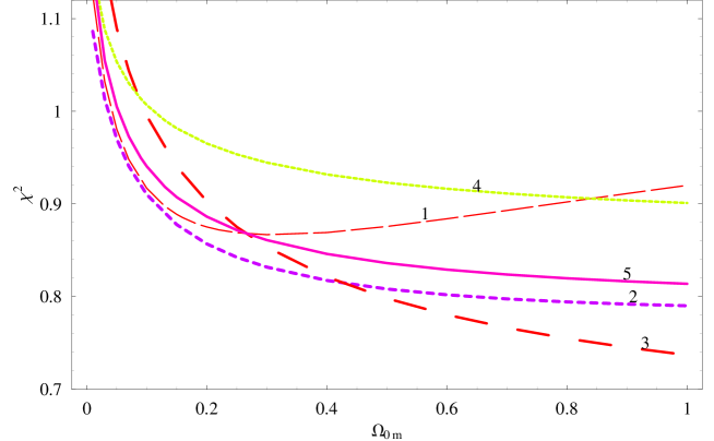
Figure 2: The variation of $\chi^{2}$ as a function of the cosmological parameter ${\Omega_{\rm m}}$ in a flat $\Lambda$CDM cosmology. Notice that only the highest quality correlation relations $1$ favors (mildly) an accelerating universe (${\Omega_{\rm m}}\simeq 0.26$). Minimization with respect to $a$, $b$ was performed for each value of ${\Omega_{\rm m}}$.

A symmetrized method may be warranted because the two variables $R_{i}$, $Q_{i}$ are not directly causative [for example, it is possible that the scatter may be dominated by hidden variables, or variables not directly measured or treated, such as the bulk Lorentz factor $\Gamma_{jet}$ (Schaefer et al. 2003, Amati et al. 2002)]. The bisector method of two ordinary least squares (Isobe et al. 1990) used in previous studies (Schaefer 2007) is an alternative symmetrized approach (for other similar approaches see Kelly 2007). That approach however ignores the measurement uncertainties during the fit which are taken into account in our symmetrized maximum likelihood method. The advantage of expressing $\chi^{2}(a,b,{\Omega_{\rm m}})$ in terms of both the calibration parameters $a$, $b$ and the cosmological parameter ${\Omega_{\rm m}}$ is that it allows either fixing ${\Omega_{\rm m}}$ and calibrating $a$, $b$ to be used for constraining other cosmological models (Schaefer 2007) or minimizing simultaneously with respect to all three parameters (Li et al. 2008b; Qi, Wang & Lu 2008). Even though the former approach may be useful as a consistency test it suffers from a circularity problem since it assumes a particular cosmological model to make the calibration and thus introduces a bias against alternative models. The later approach bypasses this circularity problem at the expense of increasing the uncertainties in the parameter determination since there are now three parameters to be fit instead of just two. Thus, in the next section we use the former approach (fixing ${\Omega_{\rm m}}$) to investigate the possible redshift dependence of the calibration parameters $a$, $b$ but we use the later approach (variable ${\Omega_{\rm m}}$) when testing for the model dependence of the calibration.

3 Results of Calibration Tests

3.1 Redshift Dependence of Calibration

In order to test if the correlation relations discussed in the previous section vary with redshift we separate the GRB samples in each case into four groups corresponding to the following redshift bins: $z\in[0,1]$, $z\in[1,2]$, $z\in[2,3]$ and $z\in[3,7]$. The number of GRBs corresponding to each correlation relation and each redshift bin is shown in Table 2.

Table 2: Number of GRBs in each redshift bin.

Correl. Type	$z\in[0,1]$	$z\in[1,2]$	$z\in[2,3]$	$z\in[3,7]$	Total
${E_{peak}}-E_{\gamma}$	10	8	4	5	27
${E_{peak}}-L$	18	15	14	17	64
${\tau_{lag}}-L$	7	13	9	9	38
$V-L$	14	15	9	13	51
${\tau_{RT}}-L$	17	15	13	17	62

We now perform a maximum likelihood fit in each group after setting ${\Omega_{\rm m}}=0.26$ obtained from the five years WMAP data (Komatsu et al. 2008), and determine the best fit calibration parameters $a$, $b$ with $1\sigma$ errors and the quality of fit expressed through the minimum $\chi^{2}$ (per degree of freedom). We use a different value for the intrinsic dispersion $\sigma_{sys}$ for each type of correlation obtained by demanding a value of $\chi^{2}$ of order 1. Thus we transfer the information about the quality from $\chi^{2}$ to $\sigma_{sys}$ (the smaller the required $\sigma_{sys}$ the better the fit). These results are shown in Table 3. We have verified that the main features of our results do not depend on the choice of ${\Omega_{\rm m}}$ in the range ${\Omega_{\rm m}}\in[0.2,0.3]$. Despite of the fact that we use the maximum likelihood method instead of linear regression used in Schaefer (2007) our results for $a_{j}$, $b_{j}$ in the full redshift range (last column of Table 3) are consistent at the $1\sigma$ level with those of Schaefer (2007).

Table 3: Best fit parameters in each redshift bin

Correlation Type	$z\in[0,1]$	$z\in[1,2]$	$z\in[2,3]$	$z\in[3,7]$	Total
${E_{peak}}-E_{\gamma}$	$b=50.56\pm 0.06$	$b=50.57\pm 0.08$	$b=50.63\pm 0.11$	$b=50.66\pm 0.15$	$b=50.60\pm 0.04$
($\sigma_{sys}=0.15$)	$a=1.56\pm 0.15$	$a=1.76\pm 0.23$	$a=0.84\pm 0.37$	$a=1.45\pm 0.26$	$a=1.56\pm 0.11$
	$\chi^{2}=1.03$	$\chi^{2}=0.65$	$\chi^{2}=0.51$	$\chi^{2}=0.34$	$\chi^{2}=0.86$
${E_{peak}}-L$	$b=52.12\pm 0.10$	$b=52.43\pm 0.12$	$b=52.61\pm 0.27$	$b=52.51\pm 0.13$	$b=52.33\pm 0.06$
($\sigma_{sys}=0.30$)	$a=1.55\pm 0.14$	$a=1.99\pm 0.33$	$a=3.08\pm 1.19$	$a=1.14\pm 0.41$	$a=1.75\pm 0.11$
	$\chi^{2}=1.11$	$\chi^{2}=0.89$	$\chi^{2}=0.40$	$\chi^{2}=0.20$	$\chi^{2}=0.84$
${\tau_{lag}}-L$	$b=51.80\pm 0.24$	$b=52.32\pm 0.14$	$b=52.32\pm 0.18$	$b=52.52\pm 0.19$	$b=52.24\pm 0.09$
($\sigma_{sys}=0.39$)	$a=-0.63\pm 0.31$	$a=-0.94\pm 0.23$	$a=-0.93\pm 0.25$	$a=-0.31\pm 0.26$	$a=-0.87\pm 0.12$
	$\chi^{2}=0.62$	$\chi^{2}=0.70$	$\chi^{2}=0.63$	$\chi^{2}=0.13$	$\chi^{2}=0.87$
$V-L$	$b=52.24\pm 0.16$	$b=52.50\pm 0.14$	$b=52.57\pm 0.20$	$b=52.69\pm 0.14$	$b=52.45\pm 0.07$
($\sigma_{sys}=0.47$)	$a=0.96\pm 0.36$	$a=2.34\pm 0.56$	$a=1.50\pm 0.54$	$a=0.03\pm 0.47$	$a=1.30\pm 0.21$
	$\chi^{2}=1.22$	$\chi^{2}=0.57$	$\chi^{2}=0.58$	$\chi^{2}=0.32$	$\chi^{2}=0.95$
${\tau_{RT}}-L$	$b=52.29\pm 0.16$	$b=52.56\pm 0.13$	$b=52.43\pm 0.13$	$b=52.59\pm 0.11$	$b=52.46\pm 0.06$
($\sigma_{sys}=0.48$)	$a=-0.92\pm 0.21$	$a=-1.05\pm 0.22$	$a=-0.81\pm 0.26$	$a=-0.43\pm 0.26$	$a=-0.92\pm 0.11$
	$\chi^{2}=0.52$	$\chi^{2}=0.27$	$\chi^{2}=0.56$	$\chi^{2}=0.19$	$\chi^{2}=0.87$

The corresponding plots of the calibration parameters $a_{j}$, $b_{j}$ vs $<z>$ (average redshift in each redshift bin) are shown in Fig. 1 for all five correlation relations. The slope of each $a_{j}(<z>)$, $b_{j}(<z>)$ with $1\sigma$ errors is also shown in Fig. 1. Notice that all slopes are consistent with zero at the $2\sigma$ level. Thus, there is no statistically significant evidence for evolution with redshift of the correlation relations. This result is to be contrasted with the result of Li (2007a, 2007b) where the Amati et al. (2002) relation $E_{peak}-E_{\gamma-iso}$ was found to have statistically significant correlation with redshift for both parameters $a$ and $b$. However the latter results are under dispute by the recent paper of Ghirlanda et al. (2008). Here we use an improved variant of this relation namely $E_{peak}-E_{\gamma}$ (Ghirlanda et al. 2004) and a somewhat different GRB dataset (Schaefer 2007) and we find no statistically significant evidence for correlation of $a$, $b$ with redshift. It is also interesting to use the results of Table 3 in order to compare the five correlation relations with respect to their quality of linear fit. Since the value of the intrinsic dispersion $\sigma_{sys}$ has been adjusted for each correlation so that $\chi^{2}\simeq 1$, the comparison can not be made by simply comparing the values of $\chi^{2}$ (per degree of freedom) in each case. Instead we compare the required value of $\sigma_{sys}$. Smaller $\sigma_{sys}$ corresponds to better quality of fit. According to this test, the correlation relations are ranked according to their quality as follows:

1. ${E_{peak}}-E_{\gamma}$ ($\sigma_{sys}=0.15$),

2. ${E_{peak}}-L$ ($\sigma_{sys}=0.30$),

3. ${\tau_{lag}}-L$ ($\sigma_{sys}=0.39$),

4. $V-L$ ($\sigma_{sys}=0.47$),

5. ${\tau_{RT}}-L$ ($\sigma_{sys}=0.48$).

Clearly, the correlation relation ${E_{peak}}-E_{\gamma}$ provides significantly better fit compared to the other four relations.

Figure 3: Comparison of the distance modulus as a function of redshift, estimated by the GRB observations (solid points) and the a recent SnIa dataset of Davis et al. (open points). Last Panel: The average cross-correlation function between the GRBs and SnIa as a function of the density parameter. The different points correspond to different luminosity indicators for the current GRB data and thus to different values of the fitted model parameters. Note that we don’t plot all the error-bars in order to avoid confusion.

3.2 Model Dependence of Calibration

In order to investigate the cosmological model dependence of the calibration parameters $a_{j}$, $b_{j}$ we now allow the cosmological parameter ${\Omega_{\rm m}}$ to vary in the $\chi^{2}(a,b,{\Omega_{\rm m}})$ of eq. (5). In particular we minimize $\chi^{2}(a,b,{\Omega_{\rm m}})$ with respect to $a_{j}$, $b_{j}$ for various ${\Omega_{\rm m}}\in[0.2,0.3]$. We show $\chi^{2}_{min}({\Omega_{\rm m}})$ in Fig. 2 for all five correlation relations. As shown in Fig. 2 the best correlation relation (${E_{peak}}-E_{\gamma}$) develops a minimum with respect to ${\Omega_{\rm m}}$ at ${\Omega_{\rm m}}=0.30^{+1.60}_{-0.25}$ (the $1\sigma$ error is obtained by demanding $\chi^{2}<\chi^{2}_{min}+3.53/N$ corresponding to maximum likelihood minimization with three parameters). On the other hand, the $\chi^{2}$ for other four correlation relations are monotonic with respect to ${\Omega_{\rm m}}$ and seem to favor a flat matter dominated universe. We attribute this behavior to the large intrinsic scatter inherent in these correlation relations. The fact that these relations favor large ${\Omega_{\rm m}}$ may explain the fact that the best fit ${\Omega_{\rm m}}$ obtained by Schaefer (2007) using a combination of all five correlation was somewhat larger (${\Omega_{\rm m}}\simeq 0.39$) than the corresponding values obtained using other more robust cosmological tests. We thus argue that the mixing of the best quality correlation with the other four correlations plagued with large scatter may lead to misleading results and perhaps should be avoided. To this end, it is interesting to mention that systematic effects introduced by the flux limits of the GRB surveys (Lloyd et al. 2000) could potentially affect the above statistical results. In order to check such a possibility, in the next section we perform a direct comparison between the GRBs with the SnIa data.

4 GRBs versus SnIa

An alternative model independent test of the GRBs as standard candles is their direct comparison with the best cosmological standard candles available namely SnIa. Thus we perform a cross-correlation analysis in the distance modulus space in the redshift range $z\in[0.17,1.75]$. The cross-correlation between two samples (in our case GRB and SnIa) is typically defined by the following estimator (Peebles 1973; Efstathiou et al. 1991):

$$\xi(\mu)=f\frac{N_{GG}}{N_{GS}}-1,$$ (10)

where $N_{GG}$ and $N_{GS}$ is the number of GRB-GRB and GRB-SnIa pairs respectively in the interval $[\mu,\mu+\delta\mu]$. For a $\xi(\mu)=0$ there is not any correlation between the two populations. Having known (from the $\chi^{2}-$analysis) the calibrations for every $L$ or $E_{\gamma}$, we can also derive [see eqs (1) and (2)] the corresponding distance modulus $\mu(z)=5{\rm log}d_{L}(z)+25$. Note that $\delta\mu$ is set at 0.75 which corresponds to 10 number of bins. The robustness of our results was tested using different bins (spanning from 7 to 15) and we found very similar statistical results. In the above relation $f$ is the normalization factor $f=2N_{S}/(N_{G}-1)$ where $N_{G}$ and $N_{S}$ are the total number of GRB and SnIa entries respectively. The uncertainty in $\xi(\mu)$ is estimated as $\sigma_{\xi}=\sqrt{(1+\xi(\mu))/N_{GS}}$ (Peebles 1973). To this end, we estimate the average cross-correlation function, which is given by:

$$\xi_{c}=N^{-1}_{b}\sum_{i=1}^{N_{b}}\xi^{i}(\mu)$$ (11)

where $N_{b}$ is the number of bins used ($N_{b}=10$).

In this paper we utilize the sample of 192 standard candles (supernovae) of Davis et al. (2007) in the $0.016\leq z\leq 1.755$. Due to the fact that the GRB observations extend beyond $z\geq 0.17$, we apply our statistical analysis to the following redshift interval $0.170\leq z\leq 1.755$. In this case, the SnIa subsample contains 146 entries, ${E_{peak}}-E_{\gamma}$ contains 17 entries, ${E_{peak}}-L$ contains 32 entries, ${\tau_{lag}}-L$ contains 19 entries, $V-L$ contains 28 entries and ${\tau_{RT}}-L$ contains 31 entries.

In Fig.3 we compare the estimated GRB distance moduli (solid points) with those derived by the SnIa data (open points) as a function of redshift. Performing, a standard Kolmogorov-Smirnov (KS) test to the distance moduli we find that the probability of consistency between GRBs and SnIa using the $E_{peak}-E_{\gamma}$ relation is ${\cal P}_{KS}\sim 0.4$. Clearly, there is a strong indication that the $E_{peak}-E_{\gamma}$ relation traces well the SnIa regime, a fact corroborated also by the cross-correlation test between GRBs and SnIa, which gives an average cross-correlation function of $0.38\pm 0.09$ for $\Omega_{\rm m}=0.30$ or a $\sim 4\sigma$ correlation signal. Notice that the cross-correlation analysis was performed for each value of $\Omega_{\rm m}$. Doing so, in the last panel of Fig.3 we present, for each GRB subsample, the average cross-correlation function $\xi_{c}$ as a function of $\Omega_{\rm m}$. It becomes clear that the best GBR tracer of the SnIa regime is the $E_{peak}-E_{\gamma}$ relation. Interestingly, the cross correlation function peaks at $\Omega_{\rm m}\simeq 0.15$ and $\Omega_{\rm m}\simeq 0.30$ respectively. However, due to small number statistics the $E_{peak}-E_{\gamma}$ test (17 entries) provides much weaker constraints on ${\Omega_{\rm m}}$ than current SnIa data. On the other hand, the $\tau_{lag}-L$ gives a relatively good correlation signal up to $\Omega_{\rm m}\leq 0.3$ although, the amplitude of the cross-correlation function decreases rapidly as a function of $\Omega_{\rm m}$ than the $E_{peak}-E_{\gamma}$ case. Finally, the $\tau_{RT}-L$, $E_{peak}-L$ and $V-L$ relations seem to fluctuate around zero (in agreement with the $\chi^{2}$ minimization results of Fig. 2).

5 Conclusions

We have investigated the robustness of the current GRB data calibrated as luminosity indicators with respect to two sources of biases: evolution of the calibration with redshift and dependence of the calibration on the assumed cosmological model. We have found no statistically significant evidence for evolution of the calibration parameters $a$, $b$ with redshift for any of the luminosity indicator correlations considered. However, our statistical results do not exclude the possibility of correlation to be discovered in the future based on better GRB data. We have also found that the correlation ${E_{peak}}-E_{\gamma}$ has two important advantages over the other four correlations considered:

• Its intrinsic scatter $\sigma_{sys}$ is less than half of the corresponding scatter of the other four correlations

• It can pick up the accelerating expansion of the universe in a model independent way [it has a clear global minimum of $\chi^{2}(a,b,{\Omega_{\rm m}})$ at ${\Omega_{\rm m}}\simeq 0.3$]

• It traces relatively well the SnIa regime.

However, even the best GRB luminosity indicator correlation is currently not competitive with other cosmological probes of the acceleration expansion since the cosmological parameter $1\sigma$ errors (${\Omega_{\rm m}}=0.30^{+1.60}_{-0.25}$) are more than an order of magnitude larger than the corresponding errors obtained eg using SnIa standard candles and other geometrical probes (${\Omega_{\rm m}}=0.267^{+0.028}_{-0.018}$). Therefore, even though the GRB data are currently not competitive with other cosmological probes of the accelerating expansion of the universe this may well change in the future if the ${E_{peak}}-E_{\gamma}$ GRB dataset expands well beyond its current status consisting of only 27 datapoints.

References

- [] Amati, L., et al., 2002, ApJ, 390, 81
- [] Amati, L., et al., 2008, arXiv:0805.0377, MNRAS, submitted
- [] Astier, P. et al., 2006, A&A, 447, 31
- [] Bertolami, O., &, Tavares Silva, P., 2006, MNRAS, 365, 1149
- [] Bertschinger, E., 2006, ApJ, 648, 797
- [] Boisseau, B, Esposito-Farese, G., Polarski D., &, Starobinsky, A. A., 2000, Phys. Rev. Lett. 85, 2236
- [] Butler, N. R., Kocevski, D., Bloom, J. S., &, Curtis, J. L, 2007, ApJ, 671, 656
- [] Butler, N. R., Kocevski, D., &, Bloom, J. S., 2008, submitted to ApJ, (arXiv0802.3396)
- [] Caldwell, R., Cooray, A., &, Melchiorri, A., 2007, Phys. Rev. D, 76, 023507
- [] Dai, Z. G., Liang, E. W., &, Xu, D., 2004, ApJ, 612, L101
- [] Davis, T. M., et al., 2007, ApJ, 666, 716
- [] Demianski, M., Piedipalumbo, E., Rubano, C., &, Tortora, C., 2006 A&A, 454, 55
- [] Di Girolamo, T., Catena, R., Vietri, M., &, Di Sciascio, G., 2005, JCAP, 0504, 008
- [] Efstathiou, G., Bernstein, G., Katz, N., Tyson, J. A., &, Guhathakurta, P., 1991, ApJ, 380, L47
- [] Fenimore, E. E., &, Ramirez-Ruiz, E., 2000, (arXiv:astro-ph/0004176)
- [] Firmani, C., Ghisellini, G., Avila-Reese, V., &, Ghirlanda, G., 2006, MNRAS, 370, 185
- [] Frail, D. A., et al., 2001, ApJ, 562, L55
- [] Ghirlanda, G., Ghisellini, G., &, Lazzati, D., 2004, ApJ, 616, 331
- [] Ghirlanda, G., Ghisellini, G., &, Firmani, C., 2006, New J. Phys., 8, 123
- [] Ghirlanda, G., Nava, L., Ghisellini, G., Firmani, C., &, Cabrera, J. I., 2008, MNRAS, 387, 319
- [] Heavens, A. F., Kitching, T. D., &, Verde, L., 2007, MNRAS, 380, 1029
- [] Hooper, D., &, Dodelson, S., 2007, Astropart. Phys., 27, 113
- [] Isobe, T., Feigelson, E. D., Akritas, M. G., &, Babu, G. J., 1990, ApJ, 364, 104
- [] Jain B., &, Zhang, P., 2007, (arXiv:0709.2375)
- [] Kawai, N., et al., 2006, Nature, 440, 184
- [] Kelly, B. C., 2007, ApJ, 665, 1489
- [] Komatsu, E., et al., 2008, ApJS, submitted, (arXiv:0803.0547)
- [] Lazkoz, R., Nesseris, S., &, Perivolaropoulos, L., 2007, (arXiv:0712.1232)
- [] Li, L-X., 2007a, MNRAS, 379, L55
- [] Li, L-X, 2007b, To appear in the proceedings of ’The Next Decade of GRB afterglows’, Amsterdam (arXiv:0705.4401)
- [] Li, H., Su, M., Fan, Z., Dai, Z., &, Zhang, X., 2008a, Phys. Lett. B, 658, 95
- [] Li, H., Xia, Jun-Qing, Liu, J., Zhao, Gong-Bo, Fan, Zu-Hui,&, Zhang, X. 2008b, ApJ, 680, 92
- [] Lloyd, N. M., Petrosian, V., Mallozzi, R. S., 2000, ApJ, 534, 227
- [] Mosquera Cuesta, H. J., Dumet, H. M.,&, Furlanetto, C., 2007, (arXiv:0708.1355)
- [] Nesseris, S., &, Perivolaropoulos, L., 2006, Phys. Rev. D, 73, 103511
- [] Nesseris, S., &, Perivolaropoulos, L., 2007, Phys. Rev. D, 75, 023517
- [] Nesseris, S., &, Perivolaropoulos, L., 2008, Phys. Rev. D, 77, 023504
- [] Norris, J. P., Marani, G. F., &, Bonnell, J. T., 2000,ApJ, 534, 248
- [] Padmanabhan, T., 2003, Phys. Rept., 380, 235
- [] Peebles, P. J. E., 1973, ApJ, 185, 413
- [] Perivolaropoulos, L, 2005, JCAP, 0510, 001
- [] Perlmutter, S., et al., 1999, ApJ, 517, 565
- [] Percival, W. J., Cole, S., Eisenstein, D. J., Nichol, R. C., Peacock, J. A., Pope, A. C., &, Szalay, A. S., 2007, MNRAS, 381, 1053
- [] Piran, T., 2004, Rev. Mod. Phys., 76, 1143
- [] Qi, S., Wang, F. Y.,&, Lu, T., 2008, A&A, 483, 49
- [] Rhoads, J. E., 1999, ApJ, 525, 737
- [] Reichart, D. E., Lamb, D. Q., Fenimore, E. E., Ramirez-Ruiz, E., Cline, T. L., Hurley, K., 2001, ApJ, 552, 57
- [] Riess, A. G., et al., 1998, AJ, 116, 1009
- [] Sari, R., Piran, T., &, Halpern, J. P., 1999, ApJ, 519, L17
- [] Schaefer, B. E., 2003, ApJ, 583, L67
- [] Schaefer, B. E., 2007, ApJ, 660,16
- [] Tegmark, M., et al., 2006, Phys. Rev. D., 74, 123507
- [] Vishwakarma, R.G., 2007, Int. J. Mod. Phys. D 16, 1641. [arXiv:astro-ph/0511628].
- [] Wang, F. Y., &, Dai, Z. G., 2006, MNRAS, 368,371
- [] Wang, S., Hui, L., May, M., &, Haiman, Z., 2007 Phys. Rev. D, 76, 063503
- [] Zhang, Z. B.&, Xie, G. Z., 2007, (arXiv:0711.1411)
- [] Zhang, B., &, Meszaros, P., 2004, Int. J. Mod. Phys. A, 19, 2385