Frustration and entanglement in the $t_{2g}$ spin–orbital model on a triangular lattice:
valence–bond and generalized liquid states

Abstract

We consider the spin–orbital model for a magnetic system with singly occupied but triply degenerate $t_{2g}$ orbitals coupled into a planar, triangular lattice, as would be exemplified by NaTiO₂. We investigate the ground states of the model for interactions which interpolate between the limits of pure superexchange and purely direct exchange interactions. By considering ordered and dimerized states at the mean–field level, and by interpreting the results from exact diagonalization calculations on selected finite systems, we demonstrate that orbital interactions are always frustrated, and that orbital correlations are dictated by the spin state, manifesting an intrinsic entanglement of these degrees of freedom. In the absence of Hund coupling, the ground state changes from a highly resonating, dimer–based, symmetry–restored spin and orbital liquid phase, to one based on completely static, spin–singlet valence bonds. The generic properties of frustration and entanglement survive even when spins and orbitals are nominally decoupled in the ferromagnetic phases stabilized by a strong Hund coupling. By considering the same model on other lattices, we discuss the extent to which frustration is attributable separately to geometry and to interaction effects.

I Introduction

Frustration in magnetic systems may be of geometrical origin, or may arise due to competing exchange interactions, or indeed both.Diep For quantum spins, frustration acts to enhance the effects of quantum fluctuations, leading to a number of different types of magnetically disordered state, among which some of the more familiar are static and resonating valence–bond (VB) phases. A further form of solution in systems with frustrated spin interactions is the emergence of novel ordered states from a highly degenerate manifold of disordered states, and the mechanism for their stabilization has become known simply as “order–by–disorder”.Diep ; Faz99 Many materials are now known whose physical properties could be understood only by employing microscopic models with frustrated spin interactions in which some of these theoretical concepts operate.

A different and still richer situation occurs in the class of transition–metal oxides or fluorides with partly filled $3d$ orbitals and near–degeneracy of active orbital degrees of freedom. In undoped systems, large Coulomb interactions on the transition–metal ions localize the electrons, and the low–energy physics is that of a Mott (or charge–transferZsa85 ) insulator. Their magnetic properties are described by superexchange spin–orbital models, derived directly from the real electronic structure and containing linearly independent but strongly coupled spin and orbital operators.Ole05 Such models emerge from the charge excitations which involve various multiplet states,Kug73 ; Cas78 in which ferromagnetic (FM) and antiferromagnetic (AF) interactions, as well the tendencies towards ferro–orbital (FO) and alternating orbital (AO) order, compete with each other. This leads to a profound, intrinsic frustration of spin–orbital exchange interactions, which occurs even in case of only nearest–neighbor interactions for lattices with unfrustrated geometry, such as the square and cubic lattices.Fei97 The underlying physics is formulated in the Goodenough–Kanamori rules,Goode which imply that the two types of order are complementary in typical situations: AO order favors a FM state while FO order coexists with AF spin order. Only recently have exceptions to these rules been noticed, Ole06 and the search for such exceptions, and thus for more complex types of spin–orbital order or disorder, have become the topic of much active research.

A case study for frustration in coupled spin–orbital systems is provided by the one–dimensional (1D) SU(4) model.Li98 One expects a priori no frustration in one dimension and with only nearest–neighbor interactions. However, spin and orbital interactions, the latter formulated in terms of pseudospin operators, appear on a completely symmetrical footing for every bond, and favor respectively AF and AO ordering tendencies, which compete with each other. In fact a low–energy but magnetically disordered spin state also frustrates the analogous pseudospin–disordered state, and conversely. This competition results in strong, combined spin–orbital quantum fluctuations which make it impossible to separate the two subsystems, and it is necessary to treat explicitly entangled spin–pseudospin states.Ole06 ; Pss07 While in one sense this may be considered as a textbook example of frustration and entanglement, the symmetry of the entangled sectors is so high that joint spin–pseudospin operators are as fundamental as the separate spin and pseudospin operators, forming parts of a larger group of elementary (and disentangled) generators. The fact that the 1D SU(4) model is exactly solvable also results in fundamental symmetries between the intersite correlation functions for the spin and orbital (and spin–orbital) sectors.Fri99 We return below to a more detailed discussion of entanglement and its consequences. Although indicative of the rich underlying physics (indeed, unconventional behavior has been identified for the SU(4) Hamiltonian on the triangular lattice,Li98 ; rpmfm ) the implications of this model are rather limited because it does not correspond to the structure of superexchange interactions in real correlated materials.

Realistic superexchange models for perovskite transition–metal oxides with orbital degrees of freedom have been known for more than three decades,Kug73 ; Cas78 but the intrinsic frustrating effects of spin–orbital interactions have been investigated only in recent years.Fei97 ; Kha00 A primary reason for this delay was the complexity of the models and the related quantum phenomena, which require advanced theoretical methods beyond a straightforward mean–field theory. The structure of spin–orbital superexchange involves interactions between SU(2)–symmetric spins $\{{\vec{S}}_{i},{\vec{S}}_{j}\}$ on two nearest–neighbor transition–metal ions $\{i,j\}$, each coupled to orbital operators $\{{\vec{T}}_{i},{\vec{T}}_{j}\}$ which obey only much lower symmetry (at most cubic for a cubic lattice), and its general form isOle05

$${\cal H}_{J}=J\sum_{\langle ij\rangle\parallel\gamma}\left\{{\hat{J}}_{ij}^{(\gamma)}\left({\vec{S}}_{i}\cdot{\vec{S}}_{j}\right)+{\hat{K}}_{ij}^{(\gamma)}\right\}.$$ (1)

The energy scale $J$ is determined (Sec. II) by the interaction terms and effective hopping matrix elements between pairs of directional $e_{g}$ orbitals [$(dd\sigma)$ element] or $t_{2g}$ orbitals [$(dd\pi)$ element] The orbital operators ${\hat{J}}_{ij}^{(\gamma)}$ and ${\hat{K}}_{ij}^{(\gamma)}$ specify the orbitals on each bond $\langle ij\rangle\parallel\gamma$, which participate in $d^{n}_{i}d^{n}_{j}\rightleftharpoons d^{n+1}_{i}d^{n-1}_{j}$ virtual excitations, and thus have the symmetry of the lattice. The form of the orbital operators depends on the valence $n$, on the type ($e_{g}$ or $t_{2g}$) of the orbitals and, crucially, on the bond direction in real space.Bri04 It is clear from Eq. (1) that individual terms in the Hamiltonian ${\cal H}_{J}$ can be minimized for particularly chosen spin and orbital configurations,Ole05 but in general the structure of the orbital operators ensures a competition between the different bonds.

This directional nature is the microscopic origin of the intrinsic frustration mentioned above, which is present even in the absence of geometrical frustration. Both spin and orbital interactions are frustrated, making long–range order more difficult to realize in either sector, and enhancing the effects of quantum fluctuations. Quite generally, because insufficient (potential) energy is available from spin or orbital order, instead the system is driven to gain (kinetic) energy from resonance processes, promoting phases with short–range dynamical correlations and leading naturally to spin and/or orbital disorder. Disordering tendencies are particularly strong in highly symmetric systems, which for crystalline materials means cubic and hexagonal structures. Among possible magnetically disordered phases for spin systems, tendencies towards dimer formation are common in the regime of predominantly AF spin interactions, and new phases with VB correlations occur. This type of physics was discussed first for $e_{g}$ orbitals on the cubic lattice,Fei97 and, in the context of BaVS₃, for one version of the problem of $t_{2g}$ orbitals on a triangular lattice.rmkzmpfbf The same generic behavior has since been found for $t_{2g}$ orbitals on the cubic lattice,Hor03 $e_{g}$–orbital systems on the triangular lattice,Ver04 ; Mil07 and for $t_{2g}$ orbitals in the pyrochlore geometry.Mat04 ; Mat05 By analogy with spin liquids, the orbital–liquid phaseDiep has been introduced for systems with both $e_{g}$Fei97 ; Fei05 and $t_{2g}$Kha00 ; Kha05 orbital degrees of freedom. The orbital liquid is a phase in which strong orbital fluctuations restore the symmetry of the orbital sector, in the sense that the instantaneous orbital state of any site is pure, but the time average is a uniform occupation of all available orbital states. We note that in the discussion of orbital liquids in $t_{2g}$ systems,Kha00 ; Kha05 it was argued that the spin sector would be ordered. To date little is known concerning the behavior of orbital correlations in an orbital liquid, the possible instabilities of the orbital liquid towards dimerized or VB phases, or its interplay with lattice degrees of freedom.

One possible mechanism for the formation of an orbital liquid state is the positional resonance of VBs. There has been considerable recent discussion of spin–orbital models in the continuing search for a realistic system realizing such a resonating VB (RVB) state,Mil07 including in a number of the references cited in the previous paragraph. While the RVB state was first proposed for the $S=\frac{1}{2}$ Heisenberg model on a triangular lattice,rfa extensive analysis of spin–only models has not yet revealed a convincing candidate system, although the nearest–neighbor dimer basis has been shown to deliver a very good description of the low–energy sector for the $S=\frac{1}{2}$ Heisenberg model on a kagome lattice.rmm To date, the only rigorous proof for RVB states has been obtained in rather idealized quantum dimer models (QDMs),Rok88 most notably on the triangular lattice.Moe01 The insight gained from this type of study can, however, be usedMil07 to formulate some qualitative criteria for the emergence of an RVB ground state. These combine energetic and topological requirements, both of which are essential: the energetics of the system must establish a proclivity for dimer formation, a high quasi–degeneracy of basis states in the candidate ground manifold, and additional energy gains from dimer resonance; exact degeneracy between topological sectors (determined by a non–local order parameter related to winding of wave functions around the system) is a prerequisite to remove the competing possibility of a “solid” phase with dimer, plaquette or other “crystalline” order.rrfbim

We comment here that the “problem” of frustration, and the resulting highly degenerate manifolds of states which may promote resonance phenomena, is often solved by interactions with the lattice. Lattice deformations act to lift degeneracies and to stabilize particular patterns of spin and orbital order, the most familiar situation being that in colossal–magnetoresistance manganites.Wei04 The same physics is also dominant in a number of spinels, where electron–lattice interactions are responsible both for the Verwey transition in magnetitePie06 and for $t_{2g}$ orbital order below it, as well as for inducing the Peierls state in CuIr₂S₄ and MgTi₂O₄.Kho05 Similar phenomena are also expectedKho05 to play a role in NaTiO₂. Here, however, we will not introduce a coupling to phonon degrees of freedom, and focus only on purely electronic interactions whose frustration is not quenched by the lattice.

The spin–orbital interactions on a triangular lattice are particularly intriguing. This lattice occurs for edge–sharing MO₆ octahedra in structures such as NaNiO₂ or LiNiO₂, where the consecutive $\langle 111\rangle$ planes of Ni³⁺ ions are well separated. These two $e_{g}$–electron systems behave quite differently: while NaNiO₂ undergoes a cooperative Jahn–Teller structural transition followed by a magnetic transition at low temperatures ($T_{\rm N}=20$ K), both transitions are absent in LiNiO₂.Hol04 Possible reasons for this remarkable contrast were discussed in Ref. Rei05, , where the authors noted in particular that realistic spin–orbital superexchange neither has an SU(2)$\otimes$SU(2) structure,Ver04 nor can it ever be reduced only to the consideration of FM spin terms.Mos02 These studies showed in addition that LiNiO₂ is not a spin–orbital liquid, and that the reasons for the observed disordered state are subtle, as spins and orbitals are thought likely to order in a strictly two–dimensional (2D) spin–orbital model.Rei05

   

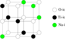
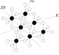
(a)                               (b)

Figure 1: (Color online) Structure of the transition–metal oxide with edge–sharing octahedra realized for NaTiO₂: (a) fragment of crystal structure, with Ti and Na ions shown respectively by black and green (grey) circles separated by O ions (open circles); (b) titanium $\langle 111\rangle$ plane with adjacent oxygen layers, showing each Ti³⁺ ion coordinated by six oxygen atoms (open circles). The directions of the Ti–Ti bonds are labeled as $XY$, $YZ$, and $ZX$, corresponding to the plane spanned by the connecting Ti–O bonds. This figure is reproduced from Ref. Rei05, , where it served to explain the structure of LiNiO₂.

The possibilities offered for exotic phases in this type of model and geometry motivate the investigation of a realistic spin–orbital model with active $t_{2g}$ orbitals, focusing first on $3d^{1}$ electronic configurations. The threefold degeneracy of the orbitals is maintained, although, as noted above, this condition may be hard to maintain in real materials at low temperatures. A material which should exemplify this system is NaTiO₂ (Fig. 1), which is composed of Ti³⁺ ions in $t_{2g}^{1}$ configuration, but has to date had rather limited experimentalHir85 ; Tak92 and theoreticalPen97 attention. Considerably more familiar is the set of triangular cobaltates best known for superconductivity in Na_xCoO₂: here the Co⁴⁺ ions have $t_{2g}^{5}$ configuration and are expected to be analogous to the $d^{1}$ case by particle–hole symmetry. The effects of doping have recently been removed by the synthesis of the insulating end–member CoO₂.Mot08 Another system for which the same spin–orbital model could be applied is Sr₂VO₄, where the V⁴⁺ ions occupy the sites of a square lattice.Ito91

The model with hopping processes of pure superexchange type was considered in the context of doped cobaltates by Koshibae and Maekawa.Kos03 These authors noted that, like the cubic system, two $t_{2g}$ orbitals are active for each bond direction in the triangular lattice, but that the superexchange interactions are very different from the cubic case because the effective hopping interchanges the active orbitals. Here we focus only on insulating systems, whose entire low–energy physics is described by a spin–orbital model. In addition to superexchange processes mediated by the oxygen ions, on the triangular lattice it is possible to have direct–exchange interactions, which result from charge excitations due to direct $d-d$ hopping between those $t_{2g}$ orbitals which do not participate in the superexchange. The ratio of these two types of interaction ($\alpha$, defined in Sec. II) is a key parameter of the model. Further, in transition–metal ionsOle05 the coefficients of the different microscopic processes depend on the Hund exchange $J_{H}$ arising from the multiplet structure of the excited intermediate $d^{2}$ state,Gri71 and we introduce

$$\eta=\frac{J_{H}}{U},$$ (2)

as the second parameter of the model. The aim of this investigation is to establish the general properties of the phase diagram in the $(\alpha,\eta)$ plane.

We conclude our introductory remarks by returning to the question of entanglement. In the analysis to follow we will show that the presence of conflicting ordering tendencies driven by different components of the frustrated intersite interactions can be related to the entanglement of spin and orbital interactions. By “entanglement” we mean that the correlations in the ground state involve simultaneous fluctuations of the spin and orbital components of the wave function which cannot be factorized. We will introduce an intersite spin–orbital correlation function to identify and quantify this type of entanglement in different regimes of the phase diagram. It has been shownOle06 that such spin–orbital entanglement is present in cubic titanates or vanadates for small values of the Hund exchange $\eta$. Here we will find entanglement to be a generic feature of the model for all exchange interactions, even in the absence of dimer resonance, and that only the FM regime at sufficiently high $\eta$, which is fully factorizable, provides a counterpoint where the entanglement vanishes.

The paper is organized as follows. In Sec. II we derive the spin–orbital model for magnetic ions with the $d^{1}$ electronic configuration (Ti³⁺ or V⁴⁺) on a triangular lattice. The derivation proceeds from the degenerate Hubbard model, and the resulting Hamiltonian contains both superexchange and direct exchange interactions. We begin our analysis of the model, which covers the full range of physical parameters, in Sec. III by considering patterns of long–ranged spin and orbital order representative of all competitive possibilities. These states compete with magnetically or orbitally disordered phases dominated by VB correlations on the bonds, which are investigated in Sec. IV. The analysis suggests strongly that all long–range order is indeed destabilized by quantum fluctuations, leading over much of the phase diagram to liquid phases based on fluctuating dimers, with spin correlations of only the shortest range. In Sec. V we present the results of exact diagonalization calculations performed for small clusters with three, four, and six bonds, which reinforce these conclusions and provide detailed information about the local physical processes leading to the dominance of resonating dimer phases. In each of Secs. III, IV, and V, we conclude with a short summary of the primary results, and the reader who is more interested in an overview, rather than in detailed energetic comparisons and actual correlation functions for the different phases, may wish to read only these. Some insight into the competition and collaboration between frustration effects of different origin can be obtained by varying the geometry of the system, and Sec. VI discusses the properties of the model on related lattices. A discussion and concluding summary are presented in Sec. VII.

II Spin–orbital model

II.1 Hubbard model for $t_{2g}$ electrons

We consider the spin–orbital model on the triangular lattice which follows from the degenerate Hubbard–like model for $t_{2g}$ electrons. It contains the electron kinetic energy and electronic interactions for transition–metal ions arranged on the $\langle 111\rangle$ planes of a compound with local cubic symmetry and with the $d^{1}$ ionic configuration, and as such is applicable to Ti³⁺ or V⁴⁺ [Fig. 1(a)]. The kinetic energy is given by

$$H_{t} = -\!\!\sum_{\langle ij\rangle{\parallel}\gamma,\mu\nu,\sigma}\!\!t^{(\gamma)}_{\mu\nu}\!\left(d^{\dagger}_{i\mu\sigma}d_{j\nu\sigma}+d^{\dagger}_{j\nu\sigma}d_{i\mu\sigma}\right)\!,$$ (3)

where $d^{\dagger}_{i\mu\sigma}$ are creation operators for an electron with spin $\sigma=\uparrow,\downarrow$ and orbital “color” $\mu$ at site $i$, and the sum is made over all the bonds $\langle ij\rangle{\parallel}\gamma$ spanning the three directions, $\gamma=a,b,c$, of the triangular lattice. This notation is adopted from the situation encountered in a cubic array of magnetic ions, where only two of the three $t_{2g}$ orbitals are active on any one bond $\langle ij\rangle$, and contribute $t^{(\gamma)}_{\mu\nu}$ to the kinetic energy, while the third lies in the plane perpendicular to the $\gamma$ axis and thus hopping processes involving the $2p_{\pi}$ oxygen orbitals is forbidden by symmetry.Kha01 ; Har03 We introduce the labels $a\equiv yz$, $b\equiv xz$, and $c\equiv xy$ also for the three orbital colors, and in the figures to follow their respective spectral colors will be red, green, and blue.

(a)

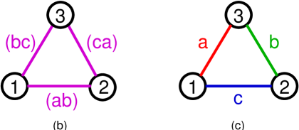
Figure 2: (Color online) (a) Schematic representation of the hopping processes in Eq. (3) which contribute to magnetic interactions on a representative bond $\langle ij\rangle$ along the $c$–axis in the triangular lattice. The $t_{2g}$ orbitals are represented by different colors (greyscale intensities). Superexchange processes involve O $2p_{z}$ orbitals (violet), and couple pairs of $a$ and $b$ orbitals (red, green) with effective hopping elements $t$, interchanging their orbital color. Direct exchange couples $c$ orbitals (blue) with hopping strength $t^{\prime}$. (b) Pairs of $t_{2g}$ orbitals active in superexchange and (c) single orbitals active in direct exchange; horizontal bonds correspond to the situation depicted in panel (a).

For the triangular lattice formed by the ions on the $\langle 111\rangle$ planes of transition–metal oxides (Fig. 1) it is also the case that only two $t_{2g}$ orbitals participate in (superexchange) hopping processes via the oxygen sites. However, unlike the cubic lattice, where the orbital color is conserved, here any one active orbital color is exchanged for the other one [Fig. 2(a)]. Using the same convention, that each direction in the triangular lattice is labeled by its inactive orbital colorKha04 $\gamma=a,b,c$, the hopping elements for a bond oriented (for example) along the $c$–axis in Eq. (3) are $t^{(c)}_{ab}=t^{(c)}_{ba}=t$, while $t^{(c)}_{aa}=t^{(c)}_{bb}=0$. In addition, and also in contrast to the cubic system, for the triangular geometry a direct hopping from one $c$ orbital to the other, i.e. without involving the oxygen orbitals, is also permitted on this bond (Fig. 2), and this element is denoted by $t^{\prime}=t^{(c)}_{cc}$. We will also refer to these hopping processes as off–diagonal and diagonal. We stress that while the lattice structure of magnetic ions is triangular, the system under consideration retains local cubic symmetry of the metal–oxygen octahedra, which is crucial to ensure that the degeneracy of the three $t_{2g}$ orbitals is preserved.

The electron–electron interactions are described by the on–site termsOle83

$$H_{int}\! = \!U\sum_{i\mu}n_{i\mu\uparrow}n_{i\mu\downarrow}+\left(U-\frac{5}{2}J_{H}\right)\!\sum_{i,\mu<\nu,\sigma\sigma^{\prime}}\!n_{i\mu\sigma}n_{i\nu\sigma^{\prime}}$$ (4)

$$- \!2J_{H}\!\sum_{i,\mu<\nu}\!{\vec{S}}_{i\mu}\!\cdot\!{\vec{S}}_{i\nu}\!+\!J_{H}\!\!\sum_{i,\mu\neq\nu}\!d^{\dagger}_{i\mu\uparrow}d^{\dagger}_{i\mu\downarrow}d_{i\nu\downarrow}d_{i\nu\uparrow},$$

where $U$ and $J_{H}$ represent respectively the intraorbital Coulomb and on–site Hund exchange interactions. Each pair of orbitals $\{\mu,\nu\}$ is included only once in the interaction terms. The Hamiltonian (4) describes rigorously the multiplet structure of $d^{2}$ ions within the $t_{2g}$ subspace, and is rotationally invariant in the orbital space.Ole83

When the Coulomb interaction is large compared with the hopping elements ($U\gg t,t^{\prime}$), the system is a Mott insulator with one $d$ electron per site in the $t_{2g}$ orbitals, whence the local constraint in the strongly correlated regime is

$$n_{ia}+n_{ib}+n_{ic}=1,$$ (5)

where $n_{i\gamma}=n_{i\gamma\uparrow}+n_{i\gamma\downarrow}$. The operators act in the restricted space $n_{i\gamma}=0,1$. The low–energy Hamiltonian may be obtained by second–order perturbation theory, and consists of a superposition of terms which follow from virtual $d_{i}^{1}d_{j}^{1}\rightleftharpoons d_{i}^{2}d_{j}^{0}$ excitations. Because each hopping process may be of either off–diagonal ($t$) [Fig. 2(b)] or diagonal ($t^{\prime}$) type [Fig. 2(c)], the Hamiltonian consists of several contributions which are proportional to three coupling constants,

$$J_{s}=\frac{4t^{2}}{U},\hskip 14.22636ptJ_{d}=\frac{4t^{\prime 2}}{U},\hskip 14.22636ptJ_{m}=\frac{4tt^{\prime}}{U}.$$ (6)

These represent in turn the superexchange term, the direct exchange term, and mixed interactions which arise from one diagonal and one off–diagonal hopping process.

We choose to parameterize the Hamiltonian by the single variable

$$\alpha=\sin^{2}\theta,$$ (7)

with

$$\tan\theta=\frac{t^{\prime}}{t},$$ (8)

which gives $J_{s}=J\cos^{2}\theta$, $J_{m}=J\sin\theta\cos\theta$, and $J_{d}=J\sin^{2}\theta$; $J$ is the energy unit, which specifies respectively the superexchange ($J=J_{s}$) and direct–exchange ($J=J_{d}$) constants in the two limits $\alpha=0$ and $\alpha=1$. The Hamiltonian

$${\cal H}=J\left\{(1-\alpha)\;{\cal H}_{s}+\sqrt{(1-\alpha)\alpha}\;{\cal H}_{m}+\alpha\;{\cal H}_{d}\right\}$$ (9)

consists of three terms which follow from the processes described by the exchange elements in Eqs. (6), each of which contains contributions from both high– and low–spin excitations.

II.2 Superexchange

Superexchange contributions to ${\cal H}$ can be expressed in the form

$${\cal H}_{s}\! = \!\frac{1}{2}\sum_{\langle ij\rangle\parallel\gamma}\Big{\{}r_{1}\Big{(}\vec{S}_{i}\!\cdot\!\vec{S}_{j}+\frac{3}{4}\Big{)}\Big{[}A_{ij}^{(\gamma)}\!+\frac{1}{2}(n_{i\gamma}+n_{j\gamma})-1\Big{]}$$ (10)

$$+r_{2}\Big{(}\vec{S}_{i}\!\cdot\!\vec{S}_{j}-\frac{1}{4}\Big{)}\Big{[}A_{ij}^{(\gamma)}\!-\frac{1}{2}(n_{i\gamma}+n_{j\gamma})+1\Big{]}$$

$$-\frac{2}{3}(r_{2}-r_{3})\Big{(}\vec{S}_{i}\!\cdot\!\vec{S}_{j}-\frac{1}{4}\Big{)}B_{ij}^{(\gamma)}\Big{\}},$$

where one recognizes a structure similar to that for superexchange in cubic vanadates,Kha00 ; Ole05 with separation into a spin projection operator on the triplet state, $(\vec{S}_{i}\cdot\vec{S}_{j}+\frac{3}{4})$, and an operator $(\vec{S}_{i}\cdot\vec{S}_{j}-\frac{1}{4})$ which is finite only for low–spin excitations. These operators are accompanied by coefficients $(r_{1},r_{2},r_{3})$ which depend on the Hund exchange parameter (2), and are given from the multiplet structure of $d^{2}$ ionsGri71 by

$$r_{1}=\frac{1}{1-3\eta},\hskip 14.22636ptr_{2}=\frac{1}{1-\eta},\hskip 14.22636ptr_{3}=\frac{1}{1+2\eta}.$$ (11)

The Coulomb and Hund exchange elements deduced from the spectroscopic data of Zaanen and SawatzkyZaa90 are $U=4.35$ eV and $J_{H}=0.59$ eV, giving a realistic value of $\eta\simeq 0.136$ for Ti²⁺ ions. For V²⁺ one findsZaa90 $U=4.98$ eV and $J_{H}=0.64$ eV, whence $\eta\simeq 0.13$, and the values for V³⁺ ions are expected to be very similar. Finally, for Co³⁺ ions,Miz96 $U=6.4$ eV and $J_{H}=0.84$ eV, giving again $\eta\simeq 0.13$. The value $\eta=0.13$ therefore appears to be quite representative for transition–metal oxides with partly filled $t_{2g}$ orbitals, whereas somewhat larger values have been found for systems with active $e_{g}$ orbitals due to a stronger Hund exchange.Ole05

The orbital operators $A_{ij}$ and $B_{ij}$ in Eq. (10) depend on the bond direction $\gamma$ and involve two active orbital colors,

$$\hskip-19.91684ptA_{ij}^{(\gamma)}\!\! = \!\!\Big{(}T_{i\gamma}^{+}T_{j\gamma}^{+}\!+T_{i\gamma}^{-}T_{j\gamma}^{-}\Big{)}\!-\!2T_{i\gamma}^{z}T_{j\gamma}^{z}+\!\frac{1}{2}n_{i}^{(\gamma)}n_{j}^{(\gamma)},$$ (12)

$$\hskip-19.91684ptB_{ij}^{(\gamma)}\! = \!\!\Big{(}T_{i\gamma}^{+}T_{j\gamma}^{-}\!+T_{i\gamma}^{-}T_{j\gamma}^{+}\Big{)}\!-\!2T_{i\gamma}^{z}T_{j\gamma}^{z}+\!\frac{1}{2}n_{i}^{(\gamma)}n_{j}^{(\gamma)}.$$ (13)

For illustration, in the case $\gamma=c$ ($\langle ij\rangle\parallel c$), the orbitals $a$ and $b$ at site $i$ are interchanged (off–diagonal hopping) at site $j$, and the electron number operator is $n_{i}^{(\gamma)}=n_{ia}+n_{ib}$. The quantity $n_{i\gamma}$ in Eq. (10) is the number operator for electrons on the site in orbitals inactive for hopping on bond $\gamma$, $n_{i\gamma}=1-n_{i}^{(\gamma)}$, or $n_{ic}$ in this example.

For a single bond, the orbital operators in Eq. (12) may be written in a very suggestive form by performing a local transformation in which the active orbitals are exchanged on one bond site, specifically $|a\rangle\rightarrow|b\rangle$ and $|b\rangle\rightarrow|a\rangle$ on bond $\gamma=c$.Kos03 Then

$$\hskip-19.91684ptA_{ij}^{(\gamma)}\!\! = \!\!2\Big{(}{\vec{T}}_{i\gamma}\cdot{\vec{T}}_{j\gamma}\!+\!\frac{1}{4}n_{i}^{(\gamma)}n_{j}^{(\gamma)}\Big{)},$$ (14)

$$\hskip-19.91684ptB_{ij}^{(\gamma)}\! = \!\!2\Big{(}\vec{T}_{i\gamma}\times\vec{T}_{j\gamma}+\frac{1}{4}n_{i}^{(\gamma)}n_{j}^{(\gamma)}\Big{)},$$ (15)

where the scalar product in $A_{ij}$ is the conventional expression for pseudospin–1/2 variables, and the cross product in $B_{ij}$ is defined as

$$\vec{T}_{i\gamma}\times\vec{T}_{j\gamma}=\frac{1}{2}(T_{i\gamma}^{+}T_{j\gamma}^{+}+T_{i\gamma}^{-}T_{j\gamma}^{-})+T_{i\gamma}^{z}T_{j\gamma}^{z}.$$ (16)

Equations (10) and (14) make it clear that for a single superexchange bond, the minimal energy is obtained either by forming an orbital singlet, in which case the optimal spin state is a triplet, or by forming a spin singlet, in which case the preferred orbital state is a triplet; we refer to these bond wavefunctions respectively as (os/st) and (ss/ot). The two states are degenerate for $\eta=0$, while for finite Hund exchange

$$E_{\rm(os/st)} = -Jr_{1},$$ (17)

$$E_{\rm(ss/ot)} = -\frac{1}{3}J\left(2r_{2}+r_{3}\right),$$ (18)

and the (os/st) state is favored. This propensity for singlet formation in the $\alpha=0$ limit will drive much of the physics to be analyzed in what follows.

Because of the off–diagonal nature of the hopping term, in the original electronic basis (before the local transformation) the orbital singlet is the state

$$|\psi_{os}\rangle=\frac{1}{\sqrt{2}}\left(|aa\rangle-|bb\rangle\right),$$ (19)

while the orbital triplet states are

$$|\psi_{ot+}\rangle = |ab\rangle,$$ (20)

$$|\psi_{ot0}\rangle = \frac{1}{\sqrt{2}}\left(|aa\rangle+|bb\rangle\right),$$ (21)

$$|\psi_{ot-}\rangle = |ba\rangle.$$ (22)

The locally transformed basis then gives a clear analogy which can be used for single bonds and dimer phases in combination with all of the understanding gained for the Heisenberg model. However, we stress here that the local transformation fails for systems with more than 1 bond in the absence of static dimer formation. This arises due to frustration, and can be shown explicitly in numerical calculations, but we will not enter into this point in more detail here. However, we take the liberty of retaining the notation of the local transformation, particularly in Sec. IV when considering dimers. Because the transformation interchanges the definitions of FO and AO configurations, we will state clearly in each section the basis in which the notation is chosen.

II.3 Direct Exchange

The direct exchange part is obtained by considering virtual excitations of active $\gamma$ orbitals on a bond $\langle ij\rangle\parallel\gamma$, which yield

$${\cal H}_{d}\! = \!\frac{1}{4}\sum_{\langle ij\rangle\parallel\gamma}\Big{\{}\Big{[}-r_{1}\Big{(}\vec{S}_{i}\!\cdot\!\vec{S}_{j}+\frac{3}{4}\Big{)}+r_{2}\Big{(}\vec{S}_{i}\!\cdot\!\vec{S}_{j}-\frac{1}{4}\Big{)}\Big{]}$$ (23)

$$\hskip 36.98866pt\times\Big{[}n_{i\gamma}(1-n_{j\gamma})+(1-n_{i\gamma})n_{j\gamma}\Big{]}$$

$$+\frac{1}{3}\left(2r_{2}+r_{3}\right)\Big{(}\vec{S}_{i}\!\cdot\!\vec{S}_{j}-\frac{1}{4}\Big{)}\;4n_{i\gamma}n_{j\gamma}\Big{\}}.$$

Here there are no orbital operators, but only number operators which select electrons of color $\gamma$ on bonds oriented along the $\gamma$–axis. When only only one active orbital is occupied [$n_{i\gamma}(1-n_{j\gamma})$], this electron can gain energy $-\frac{1}{4}J$ from virtual hopping at $\eta=0$, a number which has only a weak dependence on the bond spin state at $\eta>0$. When both active orbitals are occupied ($n_{i\gamma}n_{j\gamma}$), placing the two electrons in a spin singlet yields the far lower bond energy $-J$, and thus again one may expect much of the discussion to follow to center on dimer–based states of the extended system. Again the triplet $d^{2}$ spin excitation corresponds to the lowest energy, $(U-3J_{H})$, and only the lower two excitations involve spin singlets which could minimize the bond energy. The structure of these terms is the same as in the 1D $e_{g}$ spin–orbital model,Dag04 or the case of the spinel MgTi₂O₄.Mat04 A simplified model for the triangular–lattice model in this limit, using a lowest–order expansion in $\eta$ for the spin but not for orbital interactions, was introduced in Ref. Jac07, .

II.4 Mixed Exchange

Finally, the two different types of hopping channel may also contribute to two–step, virtual $d_{i}^{1}d_{j}^{1}\rightleftharpoons d_{i}^{2}d_{j}^{0}$ excitations with one off–diagonal ($t$) and one diagonal ($t^{\prime}$) process. The occupied orbitals are changed at both sites (Fig. 2), and as for the superexchange term the resulting effective interaction may be expressed in terms of orbital fluctuation operators. To avoid a more general but complicated notation, we write this term only for $c$–axis bonds,

$${\cal H}_{m}^{(c)}\! = \!-\frac{1}{4}\sum_{\langle ij\rangle\parallel c}\Big{[}r_{1}\Big{(}\vec{S}_{i}\!\cdot\!\vec{S}_{j}+\frac{3}{4}\Big{)}-r_{2}\Big{(}\vec{S}_{i}\!\cdot\!\vec{S}_{j}-\frac{1}{4}\Big{)}\Big{]}$$ (24)

$$\times\Big{(}T_{ia}^{+}T_{jb}^{+}+T_{ib}^{-}T_{ja}^{-}+T_{ib}^{+}T_{ja}^{+}+T_{ia}^{-}T_{jb}^{-}\Big{)},$$

where the orbital operators are

$$T_{ia}^{+} =b_{i}^{\dagger}c_{i},\hskip 19.91684ptT_{ib}^{+}=c_{i}^{\dagger}a_{i},$$

$$T_{ia}^{-} =c_{i}^{\dagger}b_{i},\hskip 19.91684ptT_{ib}^{-}=a_{i}^{\dagger}c_{i}.$$ (25)

These definitions are selected to correspond to the $\uparrow$–pseudospin components of both operators being $|b_{i}\rangle$ for $T_{ia}^{z}$ and $|c_{i}\rangle$ for $T_{ib}^{z}$. The form of the ${\cal H}_{m}^{(a)}$ and ${\cal H}_{m}^{(b)}$ terms is obtained from Eq. (24) by a cyclic permutation of the orbital indices. By inspection, this type of term is finite only for bonds whose sites are occupied by linear superpositions of different orbital colors, and creates no strong preference for the spin configuration at small $\eta$.

II.5 Limit of vanishing Hund exchange

In the subsequent sections we will give extensive consideration to the model of Eq. (9) at $\eta=0$. In this special case the multiplet structure collapses (spin singlet and triplet excitations are degenerate), one finds a single charge excitation of energy $U$, and the Hamiltonian reduces to the form

$${\cal H}(\eta=0) = J\sum_{\langle ij\rangle\parallel\gamma}\Big{\{}(1-\alpha)\Big{[}2\Big{(}\vec{S}_{i}\!\cdot\!\vec{S}_{j}+\frac{1}{4}\Big{)}\Big{(}\vec{T}_{i\gamma}\!\cdot\!\vec{T}_{j\gamma}+\frac{1}{4}n_{i}^{(\gamma)}n_{j}^{(\gamma)}\Big{)}+\frac{1}{2}(n_{i\gamma}+n_{j\gamma})-1\Big{]}$$ (26)

$$\hskip 36.98866pt+\alpha\Big{[}\Big{(}\vec{S}_{i}\!\cdot\!\vec{S}_{j}-\frac{1}{4}\Big{)}n_{i\gamma}n_{j\gamma}-\!\frac{1}{4}\Big{(}n_{i\gamma}(1-n_{j\gamma})+(1-n_{i\gamma})n_{j\gamma}\Big{)}\Big{]}$$

$$\hskip 36.98866pt-\frac{1}{4}\sqrt{\alpha(1-\alpha)}\;\Big{(}T_{i\bar{\gamma}}^{+}T_{j{\tilde{\gamma}}}^{+}+T_{i{\tilde{\gamma}}}^{-}T_{j\bar{\gamma}}^{-}+T_{i{\tilde{\gamma}}}^{+}T_{j\bar{\gamma}}^{+}+T_{i\bar{\gamma}}^{-}T_{j{\tilde{\gamma}}}^{-}\Big{)}\Big{\}},$$

which depends only on the ratio of superexchange to direct exchange ($0\leq\alpha\leq 1$). The first line of Eq. (26) makes explicit the fact that the spin and orbital sectors are completely equivalent and symmetrical at $\alpha=0$, at least at the level of a single bond. However, we will show that this equivalence is broken when more bonds are considered, and no higher symmetry emerges because of the color changes involved for different bond directions, which change the SU(2) orbital subsector. The second line of Eq. (26) emphasizes the importance of bond occupation and singlet formation at $\alpha=1$ (Sec. IIC).

In the third line of Eq. (26), the labels $\bar{\gamma}\neq{\tilde{\gamma}}$ refer to the two mixed orbital operators on each bond [Eq. (II.4)]. Orbital fluctuations are the only processes contributing to the mixed terms in this limit, where the spin state of the bond has no effect. We draw the attention of the reader to the fact that for the parameter choice $\alpha=0.5$, an electron of any color at any site has the same matrix element to hop in any direction. However, because of the different color changes involved in these processes, again the spin–orbital Hamiltonian does not exhibit a higher symmetry at this point, a result reflected in the different operator structures of superexchange and direct exchange components.

III Long–range–ordered states

In this Section we study possible ordered or partially ordered states for the Hamiltonian of Eq. (9). As explained in Sec. II, the parameters of the problem are the ratio of the direct and superexchange interactions, $\alpha$ (7), and the strength of the Hund exchange interaction, $\eta$ (2). Regarding the latter, we will discuss briefly the transition to ferromagnetic (FM) spin order for increasing $\eta$ in this framework.

The first necessary step in any analysis of such an interacting system is to establish the energies of different (magnetically and orbitally) ordered states. The high connectivity of the triangular–lattice system suggests that ordered states will dominate, and claims of more exotic ground states are justifiable only when these are shown to be uncompetitive. The calculations in this Section will be performed for static orbital and spin configurations, with the virtual processes responsible for (super)exchange as the only fluctuations. In the language of the discussion in Sec. I, fully ordered states gain only potential energy at the cost of sacrificing the kinetic (resonance) energy from fluctuation processes, which we will show in Secs. IV and V is of crucial importance here.

III.1 Possible orbital configurations

The results to follow will be obtained by first fixing the orbital configuration, either on every site or on particular bonds, and then computing the spin interaction and optimizing the spin state accordingly. While this is equivalent to the converse, the procedure is more transparent and offers more insight into the candidate phases. We limit the number of states to ordered phases with small unit cells, and the orbital states to be considered are enumerated in this subsection. For clarity we adopt the convention of Fig. 2(c) that horizontal ($c$) bonds have diagonal (direct exchange) hopping of $c$ orbitals, which are shown in blue, and off–diagonal (superexchange) hopping processes for $a$ and $b$ orbitals [Fig. 2(b)], respectively red and green; up–slanting ($a$) bonds have diagonal hopping for $a$ orbitals and off–diagonal hopping between $b$ and $c$ orbitals; down–slanting ($b$) bonds have diagonal hopping for $b$ orbitals and off–diagonal hopping between $a$ and $c$ orbitals. All Hamiltonians and energies are functions of $\alpha$ and $\eta$, as given by Eqs. (9), (10), (23), and (24). To minimize additional notation, they will be quoted in this and in the next section as functions of the single argument $\alpha$, with implicit $\eta$–dependence contained in the parameters $(r_{1},r_{2},r_{3})$. The orbital bond index $\gamma$ will also be suppressed here and in Sec. IV.

     

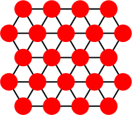
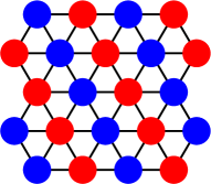
(a)                               (b)

     

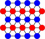
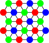
(c)                               (d)

     

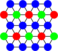
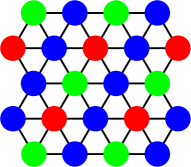
(e)                               (f)

Figure 3: (Color online) Schematic representation of possible orbital states with a single color on each site of the triangular lattice: (a) one–color state; (b) and (c) two inequivalent two–color states; (d) three–sublattice three–color state; (e) and (f) two inequivalent three–color states. The latter two configurations are degenerate with similar states where the lines of occupied $a$ and $b$ orbitals repeat rather than being staggered along the direction perpendicular to the lines of occupied $c$ orbitals. The three–sublattice state (3d) is nondegenerate ($d=1$), states (3a), (3b), and (3e) have degeneracy $d=3$, and states (3c) and (3f) have degeneracy $d=6$.

We continue to refer to the orbital type as a “color”, and begin by listing symmetry–inequivalent states where each site has a unique color. If the same orbital is occupied at every site [Fig. 3(a)], the three states with $a$, $b$, or $c$ orbitals occupied are physically equivalent (degeneracy is $d=3$). When lines of the same occupied orbitals alternate along the perpendicular direction there are two basic possibilities, which are shown in Figs. 3(b) and 3(c). These two–color states differ in their numbers of active superexchange or direct–exchange bonds, which depend on how the monocolored lines are oriented relative to the active hopping direction(s) of the orbital color. There is only one three–color configuration with equal occupations, which is shown in Fig. 3(d).

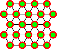
(a)

     

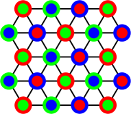
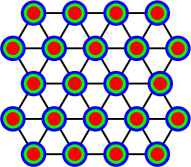
(b)                               (c)

     

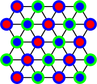
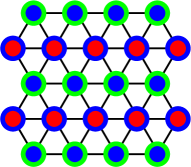
(d)                               (e)

Figure 4: (Color online) Schematic representation of possible orbital configurations with superpositions of (a) two orbitals in a two–color state, (b) three orbitals, (c) two orbitals with equal net weight, and (d) and (e) two orbitals with differing net weights of all three orbitals. State (a) has degeneracy $d=3$, states (b) and (c) have $d=1$, and the degeneracies of states (d) and (e) are $d=6$ and $d=3$.

Turning to orbital states with unequal occupations, motivated by the tendency of ${\cal H}$ to favor dimer formation in certain limits we extend our considerations to the possibility of a four–site unit cell [Figs. 3(e) and 3(f)]. More elaborate three–color unit cells are not considered. In this case the same state is obtained when the fourth site is occupied by electrons whose orbital color is any of the other three. Again this state, which breaks rotational symmetry, differs depending on its orientation relative to the active hopping axes.

States involving a superposition of either two or three orbitals at each site can be expected to allow a significantly greater variety of hopping processes. When either two or three orbital states are partially occupied at each site (we stress that the condition of Eq. (5) is always obeyed rigorously), one finds the two uniform states represented in Figs. 4(a) and 4(b). These denote the symmetric wavefunctions $|\psi_{2}\rangle=(|\phi_{a}\rangle+|\phi_{b}\rangle)/\sqrt{2}$ and $|\psi_{3}\rangle=(|\phi_{a}\rangle+|\phi_{b}\rangle+|\phi_{c}\rangle)/\sqrt{3}$ at every site, where $|\phi_{\gamma}\rangle=\gamma^{\dagger}|0\rangle$. The remaining states shown in Fig. 4 involve only two orbitals per site, but with all three orbitals partly occupied in the lattice. The average electron density per site and per orbital is $1/3$ in the state of Fig. 4(c), while in Figs. 4(d) and 4(e) it is $n_{c}=\frac{1}{2}$, $n_{a}=n_{b}=\frac{1}{4}$. The latter two states are neither unique nor (for general interactions) equivalent to each other, and represent two classes of states with respective degeneracies 3 and 6.

III.2 Ordered–state energies: superexchange

Before analyzing the different possible ordered states for any of the model parameters, we stress that the spin interactions on a given bond depend strongly on the orbital occupation of that bond. We begin with the pure superexchange model $H_{s}$ (10), meaning $\alpha=0$, for which the question of spin and orbital singlets was addressed in Sec. II.2. Here the spin and orbital scalar products $\langle{\vec{S}}_{i}\cdot{\vec{S}}_{j}\rangle$ and $\langle{\vec{T}}_{i}\cdot{\vec{T}}_{j}\rangle$ may take only values consistent with long–range order throughout the system and thus vary between $-1/4$ and $+1/4$.

For a bond on which both electrons occupy active orbitals, one has the possibility of either FO or AO states. For the FO state, $\langle{\vec{T}}_{i}\cdot{\vec{T}}_{j}\rangle=1/4=\langle{\vec{T}}_{i}\times{\vec{T}}_{j}\rangle$ and $\langle A_{ij}\rangle=\langle B_{ij}\rangle=1$, whence the terms of ${\cal H}_{s}$ can be separated into the physically transparent form

$$H_{1}^{\rm(FO)}(0) = \frac{1}{2}Jr_{1}\left(\frac{1}{2}\langle n_{i\gamma}+n_{j\gamma}\rangle\right)\left({\vec{S}}_{i}\cdot{\vec{S}}_{j}+\frac{3}{4}\right)=0,$$

$$H_{2}^{\rm(FO)}(0) = \frac{1}{2}Jr_{2}\left(2-\frac{1}{2}\langle n_{i\gamma}+n_{j\gamma}\rangle\right)\left({\vec{S}}_{i}\cdot{\vec{S}}_{j}-\frac{1}{4}\right)$$ (27)

$$= Jr_{2}\left({\vec{S}}_{i}\cdot{\vec{S}}_{j}-\frac{1}{4}\right),$$

$$H_{3}^{\rm(FO)} = \frac{1}{3}J(r_{3}-r_{2})\left({\vec{S}}_{i}\cdot{\vec{S}}_{j}-\frac{1}{4}\right),$$

specifying a net spin interaction which, because $n_{i\gamma}=0$, must be AF if any hopping processes are to occur. In the AO case, $\langle{\vec{T}}_{i}\cdot{\vec{T}}_{j}\rangle=-1/4=\langle{\vec{T}}_{i}\times{\vec{T}}_{j}\rangle$ and $\langle A_{ij}\rangle=\langle B_{ij}\rangle=0$, giving

$$H_{1}^{\rm(AO)}(0) = -\frac{1}{2}Jr_{1}\left({\vec{S}}_{i}\cdot{\vec{S}}_{j}+\frac{3}{4}\right),$$

$$H_{2}^{\rm(AO)}(0) = \frac{1}{2}Jr_{2}\left({\vec{S}}_{i}\cdot{\vec{S}}_{j}-\frac{1}{4}\right),$$ (28)

$$H_{3}^{\rm(AO)}(0) = 0,$$

and the spin interaction is constant at $\eta=0$, with only a weak FM preference emerging at finite $\eta$. We remind the reader here that the designations FO and AO continue to be based on the conventional notationFei05 obtained by a local transformation on one bond site, and in the basis of the original orbitals correspond respectively to opposite active orbitals and to equal active orbitals. Cases where only one orbital is active on a bond are by definition AO, but do contribute a finite spin interaction

$$H_{1}^{1}(0) = -\frac{1}{4}Jr_{1}\left({\vec{S}}_{i}\cdot{\vec{S}}_{j}+\frac{3}{4}\right),$$

$$H_{2}^{1}(0) = \frac{1}{4}Jr_{2}\left({\vec{S}}_{i}\cdot{\vec{S}}_{j}-\frac{1}{4}\right),$$ (29)

$$H_{3}^{1}(0) = 0,$$

which again has only a weak FM tendency at $\eta>0$. Clearly, when neither electron may hop, the bond does not contribute a finite energy.

We begin with the uniform, one–color orbital state of Fig. 3(a), meaning that all bonds are AO by the definition of the previous paragraph. In two directions both electrons are active, while in the third none are. The energy per bond is

$$E_{\rm FM}^{(3a)}(0)=-\frac{1}{3}Jr_{1}.$$ (30)

and the spin configuration is FM. However, an antiferromagnetic (AF) spin configuration on the square lattice defined by the active hopping directions has energy

$$E_{\rm AF}^{(3a)}(0)=-\frac{1}{6}J\left(r_{1}+r_{2}\right),$$ (31)

from which one observes that all spin states are degenerate at $\eta=0$. The ordered spin state spin is then FM for any finite $\eta$. We note in passing that the energy per bond for a square lattice would have the significantly lower value $-\frac{1}{2}J$ for the same ${\cal H}_{s}$ convention, by which is meant the presence of the constants $+\frac{3}{4}$ and $-\frac{1}{4}$ in Eq. (10). This result is a direct reflection of the geometrical frustration of the triangular lattice, an issue to which we return in Sec. VI.

The state of Fig. 3(b) involves one set of (alternating) AO lines with two active orbitals and two sets of (AO) lines each with one active orbital. All sets of lines favor FM order at finite $\eta$, with

$$E_{\rm FM}^{(3b)}(0)=-\frac{1}{3}Jr_{1}.$$ (32)

Here the square–lattice state which becomes degenerate at $\eta=0$, with

$$E_{\rm AF}^{(3b)}(0)=-\frac{1}{6}J\left(r_{1}+r_{2}\right),$$ (33)

is more accurately described as one with two lines of AF spins and one of FM spins [Fig. 5(a)], and will be denoted henceforth as AFF.

The state of Fig. 3(c) involves one set of FO lines with two active orbitals, one set of lines with one active orbital, one half set of AO lines with two active orbitals and one half set of inactive lines. The two–active FO lines will favor AF order, while the AO and the one–active lines will favor FM order only at $\eta>0$, giving

$$E_{\rm AFF}^{(3c)}(0)=-\frac{1}{72}J\;(9r_{1}+11r_{2}+4r_{3})$$ (34)

from the AFF configuration, but with 2 equivalent directions for the FM line. At $\eta=0$ the energy is again $-\frac{1}{3}J$. Both $E_{\rm AF}^{(3b)}(0)$ and $E_{\rm AFF}^{(3c)}(0)$ can be regarded as the energy of an unfrustrated system, in the sense that the spin order enforced in any one direction by the orbital configuration at no time denies the system the ability to adopt the energy–minimizing configuration in other directions. However, at finite $\eta$ the configurations shown in Figs. 3(b) and 3(c) will be penalized relative to the uniform (AO) order of Fig. 3(a) due to the presence of AF bonds.

     

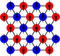
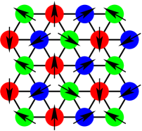
(a)                               (b)

Figure 5: (Color online) Spin configurations minimizing the total energy of the superexchange Hamiltonian ${\cal H}_{s}$ ($\alpha=0$) for given fixed patterns of orbital order: (a) AFF state for the orbital ordering pattern of Fig. 3(c), showing how the FM line is selected by the direction (here $b$) giving zero frustration; (b) 60–120^∘ ordered spin configuration minimizing the total energy for the orbital ordering pattern of Fig. 3(d).

We insert here an important observation: the orbital state of Fig. 3(c) also admits the formation of 1D AF Heisenberg spin chains on the FO ($b$–axis) lines. The energy per bond of such a state includes constant interchain contributions which are independent of the spin state ($\langle{\vec{S}}_{i}\cdot{\vec{S}}_{j}\rangle=0$) on these bonds. Of these interchain bonds, 1/4 are FO with two active orbitals and 1/2 have one active orbital. One finds

$$E_{\rm 1D}^{(3c)}(0)=-\frac{1}{9}J\ln 2\;(2r_{2}+r_{3})-\frac{1}{24}J(3r_{1}+r_{2}),$$ (35)

which gives $E_{\rm 1D}^{(3c)}(0)=-0.3977J$ at $\eta=0$. This energy is significantly lower than that of an ordered magnetic state, a result showing that the kinetic energy gained from resonance processes on the chains is far more significant than minimal potential energy gain obtainable from an ordering of the magnetic moments on the active interchain bonds which are active, and thus provides strong evidence in favor of the hypothesis that any ordered state will “melt” to a quantum disordered one in this system. We will return to this issue below.

For the two–color superposition [Fig. 4(a)], one set of bonds always has two active orbitals, but with equal probability of being FO or AO, while the other two sets of bonds have a 1/4 probability of having two active orbitals, which are FO, or a 1/2 probability of having one active orbital (and a 1/4 probability of having none). Under these circumstances, the net system Hamiltonian can be expressed by summing over all the possible orbital states, although this is not necessarily a useful exercise when the spin state may not be isotropic. By inserting the three most obvious ordered spin states, FM, AF (meaning here the AF state of the triangular lattice with 120^∘ bond angles and $\langle{\vec{S}}_{i}\cdot{\vec{S}}_{j}\rangle=-\frac{1}{8}$) and AFF, the candidate energies are

$$E_{\rm FM}^{(4a)}(0) = -\frac{1}{6}Jr_{1},$$ (36)

$$E_{\rm AF}^{(4a)}(0) = E_{\rm AFF}^{(4a)}(0)\;=\;-\frac{1}{48}J\;(5r_{1}+7r_{2}+2r_{3}).$$

The coincidence for the results for the AF and AFF ordered states in this case is an accidental degeneracy. The final energy $E_{\rm AF(F)}^{(4a)}=-\frac{7}{24}J$ at $\eta=0$ shows that both states are compromises, and it is not possible to put all bonds in their optimal spin state simultaneously. This arises because of the presence of two–active FO components in all three lattice directions, and will emerge as a quite generic feature of superposition states, albeit not one without exceptions.

In general there is no compelling reason (given by ${\cal H}$ for any value of $\alpha$) to expect that two–color superpositions of this type may be favorable. While the 120^∘ state of a triangular–lattice antiferromagnet is one compromise within a space of SU(2) operators, this type of symmetry–breaking is not relevant within the orbital sector, where there are three colors and the two–color subsector of active orbitals in the $\alpha=0$ limit changes as a function of the bond orientation.

In the equally weighted three–color state [Fig. 3(d)], all bonds are FO and it is easy to show that 1/3 of them (arranged as isolated triangles) have two active orbitals while the other 2/3 have one active orbital. The two–active bonds favor AF order while the one–active bonds have only a weak preference for FM order at finite $\eta$. In this case the problem becomes frustrated and is best resolved by a kind of AF state on the triangular lattice where the strong triangles have 120^∘ angles and alternating triangles have spins either all pointing in or all pointing out [Fig. 5(b)]; then 2/3 of the intertriangle bonds have 60^∘ angles while the other 1/3 have 120^∘ angles. The energy of this state is

$$E^{(3d)}(0)=-\frac{1}{144}J\;(19r_{1}+17r_{2}+6r_{3}),$$ (37)

and $E^{(3d)}(0)=-\frac{7}{24}J$ at $\eta=0$, a value again inferior to the optimal energy due to the manifest spin frustration.

In the state of Fig. 3(e), the only AO bonds (1/6 of the total) contain inactive orbitals. Of the remaining bonds, 3/6 have two active FO orbitals (in all three directions) and 2/6 have one active orbital. Once again the system is composed of strongly coupled triangles, but this time in a square array and with strong coupling in their basal direction by one set of two–active FO bonds. Possible competitive spin–ordered states would be AF or AFF, with energies

$$E_{\rm AF}^{(3e)}(0) = -\frac{1}{96}J\;(5r_{1}+15r_{2}+6r_{3}),$$ (38)

$$E_{\rm AFF}^{(3e)}(0) = -\frac{1}{288}J\;(15r_{1}+35r_{2}+16r_{3}).$$

The lowest energy is obtained for 120^∘ AF order, with the frustrated value $E_{\rm AF}^{(3e)}(0)=-\frac{13}{48}J$ for $\eta=0$.

For the state in Fig. 3(f) the FO bonds (1/6) and only 1/6 of the AO bonds have two active orbitals, while the other 2/3 of the bonds have one active orbital. In this case

$$E_{\rm FM}^{(3f)}(0) = -\frac{1}{4}Jr_{1},$$

$$E_{\rm AF}^{(3f)}(0) = -\frac{1}{96}J\;(15r_{1}+13r_{2}+2r_{3}),$$ (39)

$$E_{\rm AFF}^{(3f)}(0) = -\frac{1}{192}J\;(36r_{1}+17r_{2}+5r_{3}),$$

leading again to an AF spin state. At $\eta=0$ one has $E_{\rm AF}^{(3f)}(0)=-\frac{5}{16}J$, i.e. relatively weaker frustration.

Turning now to three–color superpositions, the “uniform” orbital state [Fig. 4(b)] is one in which on every bond there is a probability 2/9 of having two active FO orbitals, 2/9 for two active AO orbitals, 4/9 of one active orbital and 1/9 of no active orbitals. The appropriately weighted bond interaction strengths may be summed to give the net interaction, which for the three spin states considered results in the energies

$$E_{\rm FM}^{(4b)}(0) = -\frac{2}{9}Jr_{1},$$

$$E_{\rm AF}^{(4b)}(0) = -\frac{1}{36}J\;(5r_{1}+5r_{2}+r_{3}),$$ (40)

$$E_{\rm AFF}^{(4b)}(0) = -\frac{1}{81}J\;(12r_{1}+10r_{2}+2r_{3}),$$

and thus the AF state is lowest, with the value $E_{\rm AF}^{(4b)}(0)=-\frac{11}{36}J$ at $\eta=0$. While this orbital configuration does not attain the minimal energy of $-\frac{1}{3}J$, it is a close competitor: although it involves every bond, the fractional probabilities of each being in a two–active state mean that it cannot maximize individual bond contributions. However, we will see in Sec. IIID that state (4b) lies lowest over much of the phase diagram ($0<\alpha<1$) as a result of the contributions from mixed terms.

For states with unequal site occupations, in Fig. 4(c) one has a situation where on 1/3 of the bonds (arranged in separate triangles) there is a 1/4 probability of two active FO orbitals and a 1/2 probability of one active orbital, while on the remaining 2/3 of the bonds there is a 1/4 probability of two active AO orbitals, 1/4 of two active FO orbitals and 1/2 of having one active orbital. On computing the net energies for the three standard spin configurations, one obtains

$$E_{\rm FM}^{(4c)}(0) = -\frac{5}{24}Jr_{1},$$

$$E_{\rm AF}^{(4c)}(0) = -\frac{1}{192}J\;(25r_{1}+25r_{2}+8r_{3}),$$ (41)

$$E_{\rm AFF}^{(4c)}(0) = -\frac{1}{216}J\;(30r_{1}+25r_{2}+8r_{3}),$$

where the AF state with $E_{\rm AF}^{(4c)}(0)=-\frac{29}{96}J$ is the lowest at $\eta=0$. However, this state is also manifestly frustrated.

In the unequally weighted state of Fig. 4(d), the problem is best considered once again as lines of different bond types. Here 1/6 of the lines have two active orbitals (1/2 FO and 1/2 AO), 1/6 of the lines have probability 1/4 of two active orbitals (AO) and 1/2 of one active orbital, 1/3 of the lines have probability 1/4 of two active FO orbitals, 1/4 of two active AO orbitals and 1/2 of one active orbital, and the remaining 1/3 of the lines have probability 1/4 of two active orbitals (FO) and 1/2 of one active orbital. The ordered spin states yield the energies

$$E_{\rm FM}^{(4d)}(0) = -\frac{5}{24}Jr_{1},$$

$$E_{\rm AF}^{(4d)}(0) = -\frac{1}{192}J(25r_{1}+27r_{2}+6r_{3}),$$ (42)

$$E_{\rm AFF}^{(4d)}(0) = -\frac{1}{144}J(21r_{1}+17r_{2}+4r_{3}),$$

whence it is again the AF state, with a small degree of unrelieved frustration in its energy $E_{\rm AF}^{(4d)}(0)=-\frac{29}{96}J$, which lies lowest at $\eta=0$.

Finally, the state of Fig. 4(e) has the orbital pattern of Fig. 4(d) rotated in such a way that the number of active orbitals in different bond directions is changed. Now 1/3 of the bonds have probabilities 1/4 of two active orbitals (AO) and 1/2 of one active orbital, while the remaining 2/3 have probabilities 1/4 of two active orbitals (FO), 1/4 of two active orbitals (AO) and 1/2 of one active orbital. The ordered–state energies are

$$E_{\rm FM}^{(4e)}(0) = -\frac{1}{4}Jr_{1},$$

$$E_{\rm AF}^{(4e)}(0) = -\frac{1}{96}J(15r_{1}+13r_{2}+2r_{3}),$$ (43)

$$E_{\rm AFF}^{(4e)}(0) = -\frac{1}{36}J(6r_{1}+5r_{2}+r_{3}),$$

of which the AFF states lies lowest at $\eta=0$, achieving the unfrustrated value $E_{\rm AFF}^{(4e)}(0)=-\frac{1}{3}J$. That it is possible to obtain this energy in an orbital superposition is because of the absence of FO bond contributions in one direction, which can then be chosen to be FM.

The results of this section and the conclusions one may draw from them are summarized in Subsec. III.5 below.

III.3 Ordered–state energies: direct exchange

In the limit of only direct exchange, the analysis is somewhat simpler. The Hamiltonian is ${\cal H}_{d}$ of Eq. (23), and in this case a particle on any site is active in only one direction, which leads to the immediate observation that in a static orbital configuration it is never possible to have, on average, active exchange processes on more than 2/3 of the bonds. For simplicity we repeat the Hamiltonian for the two cases of AO order between sites, in which case by definition at most one of the orbitals is active, and FO order between sites, which is restricted to the case where neighboring sites have the same orbital color and the correct bond orientation. We stress that in this subsection the definitions FO and AO are entirely conventional, as the local transformation of Sec. II.2 is not relevant at $\alpha=1$, and thus the designation FO implies orbitals of the same color, and AO orbitals of different colors. One obtains the expressions

$${\cal H}^{\rm(AO)}(1) = \frac{1}{4}J\left[-r_{1}\left({\vec{S}}_{i}\cdot{\vec{S}}_{j}+\frac{3}{4}\right)\right.$$ (44)

$$\hskip 19.91684pt+r_{2}\left.\left({\vec{S}}_{i}\cdot{\vec{S}}_{j}-\frac{1}{4}\right)\right],$$

$${\cal H}^{\rm(FO)}(1) = \frac{1}{3}J\;(2r_{2}+r_{3})\left({\vec{S}}_{i}\cdot{\vec{S}}_{j}-\frac{1}{4}\right),$$ (45)

which in the $\eta=0$ limit reduce to the forms

$${\cal H}^{\rm(AO)}(1) = -\frac{1}{4}J,$$ (46)

$${\cal H}^{\rm(FO)}(1) = J\left({\vec{S}}_{i}\cdot{\vec{S}}_{j}-\frac{1}{4}\right).$$ (47)

It is clear (Sec. II) that for a single bond, the most favorable state is a spin singlet, which would contribute energy $-J$, but at the possible expense of placing all of the neighboring bonds in suboptimal states. The very strong preference for such singlet bonds means that any mean–field study of the minimal energy is incomplete without the consideration of dimerized (or valence–bond) states (Sec. IV). The analysis of this section can be considered as elucidating the optimal energies to be gained from long–ranged magnetic and orbital order on these bonds, where the optimal energy of any one is $-\frac{1}{2}J$. Also as noted in Sec. II, any active AO bond gains an exchange energy ($-\frac{1}{4}J$) simply because it does not prevent one of the two particles from performing virtual hopping processes, and this we term “avoided blocking”. In the limit of zero Hund exchange, these will give a highly degenerate manifold of all possible spin states, from which FM states are selected at finite $\eta$.

We begin again with one–color state of Fig. 3(a), which we denote henceforth as (3a). Only one set of lattice bonds has finite interactions, all FO, and therefore the system behaves as a set of AF Heisenberg spin chains with energy per bond

$$E_{\rm AF1D}^{(3a)}(1)=-\frac{1}{9}J\ln 2\;(2r_{2}+r_{3}),$$ (48)

whence $E_{\rm AF1D}^{(3a)}(1)=-0.2310J$ at $\eta=0$.

In state (3b), the FO lines do not correspond to active hopping directions. The remaining two directions then form an AO square lattice with

$$E_{\rm FM}^{(3b)}(1)=-\frac{1}{6}Jr_{1}.$$ (49)

This can be called a “pure avoided–blocking” energy. The spins are unpolarized at $\eta=0$, where all bond spin states are equivalent, but any finite $\eta$ will select FM order (hence the notation). We will see in the remainder of this section that $E=-\frac{1}{6}J$ is the optimal energy obtainable by a 2D ordered state in the direct–exchange limit ($\alpha=1$), where the net energy is generically higher than at $\alpha=0$ quite simply because there are half as many hopping channels. Thus the “melting” of such ordered states into quasi–1D states becomes clear from the outset, and can be understood due to the very low connectivity of the active hopping network on the triangular lattice.

In state (3c), one of the FO lines is active, and forms AF Heisenberg spin chains. Electrons in the other FO line are active only in a cross–chain direction, where their bonds are AO, and gain avoided–blocking energy, whence

$$E_{\rm AF}^{(3c)}(1)=-\frac{1}{12}J(2\ln 2+1)\;\;=\;\;-0.1988J$$ (50)

at $\eta=0$. As in the preceding subsection, the coherent state of each Heisenberg chain is not altered by the presence of additional electrons from other chains executing virtual hopping processes onto empty orbitals of individual sites. The spin chains remain uncorrelated and only quasi–long–range–ordered until a finite value of $\eta$, where FM spin polarization and a long–range–ordered state are favored.

In the two–color superposition (4a), 1/3 of the bonds are inactive, while on the other 2/3 one has probability 1/4 of two active electrons (FO), 1/2 of one active (AO) and 1/4 of two inactive electrons. In this case, one obtains an effective square lattice on which an AF spin configuration is favored by the FO processes, with

$$E_{\rm AF}^{(4a)}(1)=-\frac{1}{72}J\;(3r_{1}+7r_{2}+2r_{3}),$$ (51)

so again $E_{\rm AF}^{(4a)}(1)=-\frac{1}{6}J$ at $\eta=0$.

The uniform three–color state (3d) maximizes AO bonds, but 1/3 of the bonds on the lattice remain inactive. Thus

$$E_{\rm FM}^{(3d)}(1)=-\frac{1}{6}Jr_{1},$$ (52)

and Hund exchange will select the FM spin state.

The three–color state (3e) has FO lines oriented in their active direction and will, as in state (3c), form Heisenberg chains linked by bonds with AO order. While the geometry of the interchain coupling can differ depending on the orbital alignment in the inactive chains, it does not create a frustrated spin configuration and the net energy is $E_{\rm AF}^{(3e)}(1)=E_{\rm AF}^{(3c)}(1)$. The state (3f) has only inactive FO lines and so gains only avoided–blocking energy, from 2/3 of the bonds in the system, whence $E_{\rm FM}^{(3f)}(1)=E_{\rm FM}^{(3d)}(1)$.

In the uniform three–color superposition (4b), every bond has probability 1/9 of containing two active electrons (FO), 4/9 of one active electron and 4/9 of remaining inactive. For the three different ordered spin configurations considered in Subsec. III.2 the energies are

$$E_{\rm FM}^{(4b)}(1) = -\frac{1}{9}Jr_{1},$$

$$E_{\rm AF}^{(4b)}(1) = -\frac{1}{72}J\;(5r_{1}+5r_{2}+r_{3}),$$ (53)

$$E_{\rm AFF}^{(4b)}(1) = -\frac{1}{81}J\;(6r_{1}+5r_{2}+r_{3}),$$

and one finds the energy $E_{\rm AF}^{(4b)}(1)=-\frac{11}{72}J$ for the 120⁰ AF state at $\eta=0$.

The three–color state (4c) is one in which 1/3 of the bonds (arranged on isolated triangles) have probability 1/4 of being in a state with two active electrons and 1/2 of containing one active electron, while on the other 2/3 of the bonds there is simply a 1/2 probability of one active orbital. The respective energies are

$$E_{\rm FM}^{(4c)}(1) = -\frac{1}{8}Jr_{1},$$

$$E_{\rm AF}^{(4c)}(1) = -\frac{1}{192}J\;(15r_{1}+13r_{2}+2r_{3}),$$ (54)

$$E_{\rm AFF}^{(4c)}(1) = -\frac{1}{216}J\;(18r_{1}+13r_{2}+2r_{3}).$$

At $\eta=0$, the energy $E_{\rm FM}^{(4c)}(1)=-\frac{5}{32}J$ is minimized by a 120^∘ state on the triangles, which are also isolated magnetically in this limit. Finite values of $\eta$ result in FM interactions between the triangles, and a frustrated problem in the spin sector which by inspection is resolved in favor of a net FM configuration only at large $\eta$ ($\eta>0.23)$.

Finally, the three–color states (4d) and (4e) yield two possibilities in the $\alpha=1$ limit, namely where one of the minority colors is aligned with its active direction and where neither is. In the former case,

$$E_{\rm FM}^{(4d)}(1) = -\frac{5}{48}Jr_{1},$$

$$E_{\rm AF}^{(4d)}(1) = -\frac{1}{384}J\;(25r_{1}+27r_{2}+6r_{3}),$$ (55)

$$E_{\rm AFF}^{(4d)}(1) = -\frac{1}{96}J\;(7r_{1}+7r_{2}+2r_{3}),$$

and the lowest energy $E_{\rm AFF}^{(4d)}(1)=-\frac{1}{6}J$ at $\eta=0$ is given by the directionally anisotropic AFF spin configuration. This is because 1/2 of the lines, in two of the three directions, have some AF preference from their 1/4 probability of containing two active orbitals, while the third direction has no preference at $\eta=0$, and in any case favors FM spins at $\eta>0$. In the latter case, the only AF tendencies arise along lines in a single direction, but avoided–blocking energy is sufficient to exclude the possibility of a Heisenberg chain state. Here

$$E_{\rm FM}^{(4e)}(1) = -\frac{1}{8}Jr_{1},$$

$$E_{\rm AF}^{(4e)}(1) = -\frac{1}{192}J\;(15r_{1}+13r_{2}+2r_{3}),$$ (56)

$$E_{\rm AFF}^{(4e)}(1) = -\frac{1}{72}J\;(6r_{1}+5r_{2}+r_{3}),$$

whence $E_{\rm AFF}^{(4e)}(1)=-\frac{1}{6}J$ at $\eta=0$, in fact with two degenerate possibilities for the orientation of the FM line.

III.4 Ordered–state energies: $\alpha=0.5$

To illustrate the properties of the model in the presence of finite direct and superexchange contributions, i.e. at intermediate values of $\alpha$, we consider the point $\alpha=0.5$. As shown in Sec. II, there is no special symmetry at this point, because the contributions from diagonal and off–diagonal hopping remain intrinsically different. States with long–ranged orbital (and spin) order at $\alpha=0.5$ are mostly very easy to characterize, because all virtual processes, of both types, allowed by the given configuration are able to contribute in full to the net energy. For the many of the states considered in this section, the energetic calculation for $\alpha=0.5$ is merely an exercise in adding the $\alpha=0$ and $\alpha=1$ results with equal weight. Exceptions occur for superposition states gaining energy from processes contained in $H_{m}$ [Eq. (24)], and are in fact decisive here. Because these terms involve explicitly a finite density of orbitals of all three colors on the bond in question, with the active diagonal color represented on both sites, only for states (4b), (4c), and (4d), but not (4e) [Figs. 4(b–e)], will it be necessary to consider this contribution.

For state (3a), in two directions both electrons are active by off–diagonal hopping, while in the third both may hop diagonally. Diagonal hopping favors an AF spin configuration, while the off–diagonal hopping bonds have only a weak preference (by Hund exchange) for FM order. The ordered–state spin solution is then a doubly degenerate AFF state with energy per bond

$$E^{(3a)}(0.5)=-\frac{1}{72}J\;(9r_{1}+7r_{2}+2r_{3}),$$ (57)

giving $E^{(3a)}(0.5)=-\frac{1}{4}J$ at $\eta=0$. We remind the reader that the prefactor of the superexchange and direct exchange contributions is only half as large as in Subsecs. III.2 and III.3 [Eq. (9)], so the overall effect of additional hopping processes in this state is in fact an unfrustrated energy summation. We also comment that, exactly at $\eta=0$, there is no obvious preference for any magnetic order between the diagonal–hopping chains. Only at unrealistically large values of $\eta$ would the system sacrifice this diagonal–hopping energy to establish a square–lattice FM state. At finite $\eta$, the one–color orbital state represents a compromise between competing spin states preferred by the two types of hopping contribution.

State (3b) has no diagonal–hopping chains, and these processes therefore enforce only a weak preference for a FM square lattice. Because the off–diagonal hopping processes also favor FM order at finite $\eta$ (Subsec. III.2), the two types of contribution cooperate and one obtains

$$E^{(3b)}(0.5)=-\frac{1}{4}Jr_{1}.$$ (58)

State (3c) contains one half set of diagonal–hopping chains, which fall along one of the directions which in the spin state favored by the off–diagonal hopping processes could be FM or AF; this degeneracy will therefore be broken. The other half set of chains will gain only avoided–blocking energy from diagonal processes, which will take place in the FM direction and thus cause no frustration even at finite $\eta$. One obtains

$$E^{(3c)}(0.5)=-\frac{1}{144}J\left(3r_{1}+7r_{2}+2r_{3}\right),$$ (59)

and thus $E^{(3c)}(0.5)=-\frac{1}{4}J$ at $\eta=0$ from this AFF configuration. The additive contributions from superexchange and direct exchange remove the possibility that Heisenberg–chain states in either of the directions favored separately by off–diagonal (Sec. IIIB) or diagonal (Sec. IIIC) hopping could result in an overall lowering of energy.

As in Subsec. III.3, in the two–color superposition (4a) the diagonal hopping processes are optimized by an AFF spin configuration. Although this is one of the degenerate states minimizing the off–diagonal Hamiltonian, the directions of the FM lines do not match. Insertion of the four possible spin states yields

$$E_{\rm FM}^{(4a)}(0.5) = -\frac{1}{8}Jr_{1},$$

$$E_{\rm AF}^{(4a)}(0.5) = -\frac{1}{96}J\;(8r_{1}+10r_{2}+3r_{3}),$$

$$E_{\rm AFF(0)}^{(4a)}(0.5) = -\frac{1}{72}J\;(6r_{1}+7r_{2}+r_{3}),$$ (60)

$$E_{\rm AFF(1)}^{(4a)}(0.5) = -\frac{1}{144}J\;(12r_{1}+14r_{2}+3r_{3}),$$

whence the lowest final energy is $E_{\rm AF}^{(4a)}(0.5)=-\frac{7}{32}J$ at $\eta=0$. As noted in the previous sections for this spin configuration, the optimal energy for all bonds is not attainable within the off–diagonal hopping sector, and the addition of the (small) diagonal–hopping contribution causes little overall change.

The equally weighted three–color state (3d) has no lines of diagonal–hopping bonds, and in fact these contribute only avoided–blocking energy on the bonds between the strong triangles defined by the off–diagonal problem, adding to the weak propensity for FM intertriangle bonds arising only from the Hund exchange. The diagonal processes can be taken only to alter this energy, and not to promote any tendency towards an alteration of the spin state, whose energy is then

$$E^{(3d)}(0.5)=-\frac{1}{144}J\;(19r_{1}+11r_{2}+3r_{3}),$$ (61)

with $E^{(3d)}(0.5)=-\frac{11}{48}J$ at $\eta=0$.

State (3e) is already frustrated in the off–diagonal sector, and diagonal–hopping processes contribute primarily on otherwise inactive bonds without changing the frustration conditions. For the two candidate spin configurations

$$E_{\rm AF}^{(3e)}(0.5) = -\frac{1}{96}J\;(5r_{1}+12r_{2}+4r_{3}),$$

$$E_{\rm AFF}^{(3e)}(0.5) = -\frac{1}{192}J\;(11r_{1}+19r_{2}+8r_{3}),$$ (62)

a competition won by the 120^∘ AF–ordered state with $E_{\rm AF}^{(3e)}(0.5)=-\frac{7}{32}J$ at $\eta=0$.

State (3f) lacks active lines of diagonal–hopping processes, and thus the avoided–blocking energy may be added simply to the results for the off–diagonal sector, giving

$$E_{\rm FM}^{(3f)}(0.5) = -\frac{5}{24}Jr_{1},$$

$$E_{\rm AF}^{(3f)}(0.5) = -\frac{1}{192}J\;(25r_{1}+19r_{2}+2r_{3}),$$ (63)

$$E_{\rm AFF}^{(3f)}(0.5) = -\frac{5}{384}J\;(12r_{1}+5r_{2}+r_{3}),$$

or a minimum of $E_{\rm AF}^{(3f)}(0.5)=-\frac{23}{96}J$ at $\eta=0$.

In the uniform three–color superposition (4b), on every bond there is a probability 4/9 of having only off–diagonal hopping processes, 2/9 for 2 active FO orbitals and 2/9 for two active AO orbitals, a probability 1/9 of having only diagonal hopping processes, and a probability 4/9 of other processes. These last include the contributions from one active diagonal or off–diagonal electron, and mixed processes contained in the Hamiltonian ${\cal H}_{m}$ (24); none of these three possibilities favors any given bond spin configuration other than a FM orientation at finite $\eta$. The net energy contributions are

$$E_{\rm FM}^{(4b)}(0.5) = -\frac{2}{9}Jr_{1},$$

$$E_{\rm AF}^{(4b)}(0.5) = -\frac{1}{144}J\;(20r_{1}+18r_{2}+3r_{3}),$$ (64)

$$E_{\rm AFF}^{(4b)}(0.5) = -\frac{1}{54}J\;(8r_{1}+6r_{2}+r_{3}),$$

and thus the AF state is lowest, with $E_{\rm AF}^{(4b)}(0.5)=-\frac{41}{144}J$ at $\eta=0$. While this energy differs from that for the AFF spin configuration by only $\frac{1}{144}J$, its crucial property is that it lies below the value $-\frac{1}{4}J$ obtained by direct summation of the superexchange and direct–exchange contributions.

For this orbital configuration, all three spin states gain a net energy of $-\frac{1}{18}J$ at $\eta=0$ from mixed processes, and these are sufficient, as we shall see, to reduce the otherwise partially frustrated ordered–state energy to the global minimum for this value of $\alpha$. By a small extension of the calculation, the energy of the 120⁰ AF spin state may be deduced at $\eta=0$ for all values of $\alpha$, and is given by

$$E_{\rm AF}^{(4b)}(\alpha)=-\frac{1}{72}J\;\big{(}22-11\alpha+8\sqrt{\alpha(1-\alpha)}\big{)}.$$ (65)

Comparison with the value obtained by direct summation, $E=-\frac{1}{6}(2-\alpha)$, reveals that state (4b) is the lowest–lying fully spin and orbitally ordered configuration in the region $0.063<\alpha<0.983$. That this state dominates over the majority of the phase diagram is a direct consequence of its ability to gain energy from mixed processes.

The non–uniform three–color state (4c) also presents a delicate competition between spin configurations of very similar energies. From the preceding subsections, it is clear that in this case diagonal and off–diagonal processes favor different ground states, while there will also be a mixed contribution from 1/3 of the bonds. The energies of the three standard spin configurations are

$$E_{\rm FM}^{(4c)}(0.5) = -\frac{1}{12}Jr_{1},$$

$$E_{\rm AF}^{(4c)}(0.5) = -\frac{1}{384}J\;(45r_{1}+41r_{2}+10r_{3}),$$ (66)

$$E_{\rm AFF}^{(4c)}(0.5) = -\frac{1}{432}J\;(54r_{1}+41r_{2}+10r_{3}),$$

where the AF state, obtaining $E_{\rm AF}^{(4c)}(0.5)=-\frac{1}{4}J$ is the lowest at $\eta=0$.

Finally, in the three–color states (4d) and (4e), which are composed of lines of two–color sites, this delicate balance between different spin configurations persists. For configuration (4d), an AFF state with the same orientation of the FM line (along the $b$–axis) is both favored by diagonal hopping processes and competitive for off–diagonal processes. With inclusion of a small contribution due to mixed processes, the three ordered spin states have energies

$$E_{\rm FM}^{(4d)}(0.5) = -\frac{51}{288}Jr_{1},$$

$$E_{\rm AF}^{(4d)}(0.5) = -\frac{1}{768}J\;(85r_{1}+84r_{2}+18r_{3}),$$ (67)

$$E_{\rm AFF}^{(4d)}(0.5) = -\frac{1}{576}J\;(71r_{1}+59r_{2}+14r_{3}),$$

from which the AFF state minimizes the energy at $\eta=0$ with $E_{\rm AFF}^{(4d)}(0.5)=-\frac{1}{4}J$.

For state (4e), which has no mixed contribution, the orientations of the FM lines in the optimal AFF states do not match, and it is necessary, as above, to consider both possibilities when performing a full comparison. These four ordered spin states yield the energies

$$E_{\rm FM}^{(4e)}(0.5) = -\frac{3}{16}Jr_{1},$$

$$E_{\rm AF}^{(4e)}(0.5) = -\frac{1}{128}J\;(15r_{1}+13r_{2}+2r_{3}),$$

$$E_{\rm AFF(0)}^{(4e)}(0.5) = -\frac{1}{144}J\;(18r_{1}+13r_{2}+2r_{3}),$$

$$E_{\rm AFF(1)}^{(4e)}(0.5) = -\frac{1}{48}J\;(6r_{1}+4r_{2}+r_{3}),$$ (68)

among which the AF state in fact lies lowest at $\eta=0$, achieving the weakly frustrated value $E_{\rm AF}^{(4e)}(0.5)=-\frac{15}{64}J$.

III.5 Summary

Here we summarize the results of this section in a concise form. For the superexchange model ($\alpha=0$), a considerable number of 2D ordered orbital and spin states exist which return the energy $-\frac{1}{3}J$ at $\eta=0$. This degeneracy is lifted at any finite Hund exchange in favor of orbital states [(3a), (3b)] permitting a fully FM spin alignment. Most other orbital configurations introduce a frustration in the spin sector at small $\eta$, while some offer the possibility of a change of ground–state spin configuration at finite $\eta$, where $r_{1}$ exceeds the $r_{2}$ and $r_{3}$ contributions and begins to favor states with more FM bonds.

However, the value $E=-\frac{1}{3}J$ per bond remains a rather poor minimum for a system as highly connected as the triangular lattice, even if, as in the superexchange limit, active hopping channels exist only in two of the three lattice directions for each orbital color. Indeed, the limitations of the available ordering (potential) energy are clearly visible from the fact that a significantly lower overall energy is attained in systems which abandon spin order in favor of the resonance (kinetic) energy gains available in one lattice direction. The result $E_{\rm 1D}^{(3c)}(0)=-0.3977J$ is the single most important obtained in this section, and in a sense obviates all of the considerations made here for fully ordered states, mandating the full consideration of 2D magnetically and orbitally disordered phases.

In the study of ordered states, it becomes clear that the Hund exchange acts to favor FM spin alignments at high $\eta$. Because the “low–spin” states of minimal energy are in fact stabilized by quantum corrections due to AF spin fluctuations, the lowest energies at $\eta=0$ are never obtained for FM states, and therefore increasing $\eta$ drives a phase transition between states of differing spin and orbital order. We show in Fig. 6 the transitions from quasi–1D AF–correlated states at low $\eta$, for both $\alpha=0$ and $\alpha=1$, to FM states of fixed orbital and spin order (3b). The transitions occur at the values $\eta_{c}(0)=0.085$ and $\eta_{c}(1)=0.097$, indicating that FM ordered states may well compete in the physical parameter regime. We note again that the energies in the superexchange limit are lower by approximately a factor of two compared to the direct–exchange limit simply because of the number of available hopping channels.

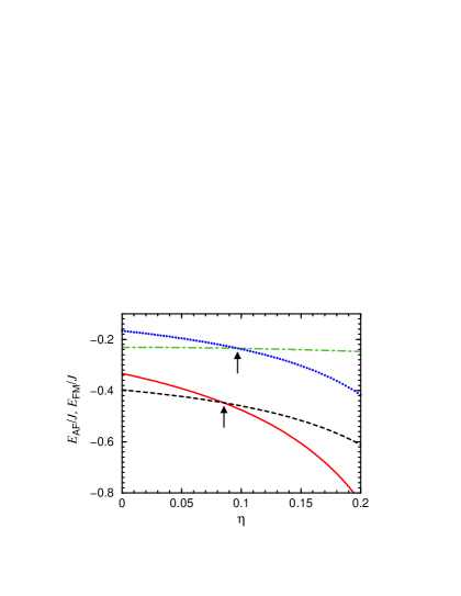
Figure 6: (Color online) Minimum energies per bond obtained for orbitally ordered phases, showing a transition as a function of Hund exchange $\eta$ from quasi–1D, AF–correlated to FM ordered spin states. For the superexchange Hamiltonian ${\cal H_{s}}$ of Sec. II ($\alpha=0$), the transition is from the quasi–1D spin state on orbital configuration (3c) [black, dashed line from Eq. (35)] to the one–color orbital state (3a) [red, solid line from Eq. (30)]. For the direct–exchange Hamiltonian ${\cal H}_{d}$ ($\alpha=1$), the transition is from the purely 1d spin state on the one–color orbital state (3a) [green, dot–dashed line from Eq. (48)] to the two–colour, avoided–blocking state (3b) [blue, dotted line from Eq. (49)]. The transitions to FM order as obtained from the mean–field considerations of this section are marked by arrows.

We note also that there is never a situation in which the spin Hamiltonian becomes that of a Heisenberg model on a triangular lattice. This demonstrates again the inherent frustration introduced by the orbital sector. However, the fact that the ordered–state energy can never be lowered to the value $E_{\rm HAF}=-\frac{3}{8}J$, which might be expected for a two–active FO situation on every bond, far less the value $-\frac{1}{2}J$ which could be achieved if it were possible to optimize every bond in some ordered configuration, can be taken as a qualitative reflection of the fact that on the triangular lattice the orbital degeneracy “enhances” rather than relieves the (geometrical) frustration of superexchange interactions (Sec. VI).

The limit of direct exchange ($\alpha=1$) is found to be quite different: the very strong tendency to favor spin singlet states, and the inherent one–dimensionality of the model in this limit (one active hopping direction per orbital color), combine to yield no competitive states with long–ranged magnetic order. Their optimal energy is very poor because of the restricted number of hopping channels, and coincides with the (“avoided–blocking”) value for the model with only AO bonds, $E=-\frac{1}{6}J$. Thus these states form part of a manifold with very high degeneracy. However, even at this level it is clear that more energy, meaning kinetic (from resonance processes) rather than potential, may be gained by forming quasi–1D Heisenberg–chain states with little or no interchain coupling and only quasi–long–ranged magnetic order. Studies of orbital configurations permitting dimerized states are clearly required (Sec. IV). Finite Hund exchange acts to favor ordered FM configurations, which will take over from chain–like states at sufficiently high values of $\eta$ (Fig. 6).

Finally, ordered states of the mixed model show a number of compromises. At $\alpha=0.5$, where the coefficients of superexchange and direct–exchange are equal, some configurations are able to return the unfrustrated sum of the optimal states in each sector when considered separately, namely $-\frac{1}{4}J$. However, superposition states, which are not optimal in either limit, can redeem enough energy from mixed processes to surpass this value, and in fact the maximally superposed configuration (4b) is found to minimize the energy over the bulk of the phase diagram. Still, the net energy of such states remains small compared to expectations for a highly connected state with three available hopping channels per orbital color. Because of the directional mismatch between the diagonal and off–diagonal hopping sectors, no quasi–1D states with only chain–like correlations are able to lower the ordered–state energy in the intermediate regime.

IV Dimer states

As shown in Sec. II, the spin–orbital model on a single bond favors spin or orbital dimer formation in the superexchange limit, and spin dimer formation in the direct–exchange limit. The physical mechanism responsible for this behavior is, as always, the fluctuation energy gain from the highly symmetric singlet state. On the basis of this result, combined with our failure to find any stable, energetically competitive states with long–ranged spin and orbital order in either limit of the model (Sec. III), we proceed to examine states based on dimers. Given the high connectivity of the triangular lattice, dimer–based states are not expected a priori to be capable of attaining lower energies than ordered ones, and if found to be true it would be a consequence of the high frustration, which as noted in Sec. I has its origin in both the interactions and the geometry. Here we consider static dimer coverings of the lattice, and compute the energies they gain due to inter–singlet correlations. The tendency towards the formation of singlet dimer states will be supported by the numerical results in Sec. V, which will also address the question of resonant dimer states.

IV.1 Superexchange model

Motivated by the fact that the spin and orbital sectors in ${\cal H}_{s}$ (10) are not symmetrical, we proceed with a simple decoupling of spin and orbital operators. Extensive research on spin–orbital models has shown that this procedure is unlikely to capture the majority of the physical processes contributing to the final energy, particularly in the vicinity of highly symmetric points of the general Hamiltonian. The results to follow are therefore to be treated as a preliminary guide, and a basis from which to consider a more accurate calculation of the missing energetic contributions. We remind the reader that the notation FO and AO used in this subsection is again that obtained by performing a local transformation on one site of every dimer. As noted in Sec. II.2, this procedure is valid for the discussion of states based on individual dimerized bonds, where it represents merely a notational convenience. For FO configurations, which in the original basis have different orbital colors, one might in principle expect that, because of the color degeneracy, there should be more ways to realize these without frustration than there are to realize AF spin configurations; however, because of the directional dependence of the hopping, we will find that this is not necessarily the case (below).

The basic premise of the spin–orbital decoupling is that if the spin (orbital) degrees of freedom on a dimer bond form a singlet state, their expectation value $\langle{\vec{S}}_{i}\cdot{\vec{S}}_{j}\rangle$ ($\langle{\vec{T}}_{i}\cdot{\vec{T}}_{j}\rangle$) on the neighboring interdimer bonds will be precisely zero. The optimal orbital (spin) state of the interdimer bond may then be deduced from the effective bond Hamiltonian obtained by decoupling. Because ${\cal H}_{s}$ depends on the number of electrons on the sites of a given bond which are in active orbitals, and this number is well defined only for the dimer bonds, the effective Hamiltonian will be obtained by averaging over all occupation probabilities. In contrast to the pure Heisenberg spin Hamiltonian, here the interdimer bonds contribute with finite energies, and the dimer distribution must be optimized. A systematic optimization will not be performed in this section, where we consider only representative dimer coverings giving the semi–quantitative level of insight required as a prelude to adding dimer resonance processes (Sec. V).

On the triangular lattice there are three essentially different types of interdimer bond, which are shown in Fig. 7). For a “linear” configuration [Fig. 7(a)], the number of electrons in active orbitals on the interdimer bond is two; for the 8 possible configurations where one dimer bond is aligned with the interdimer bond under consideration [Fig. 7(b)], the number is one on the corresponding site and one or zero with equal probability on the other; for the 14 remaining configurations where neither dimer bond is aligned with the interdimer bond [Fig. 7(c)], the number is one or zero for both sites. The number of electrons in active orbitals is then two for type (7a), two or one, each with probability 1/2, for type (7b), and two, one or zero with probabilities 1/4, 1/2, and 1/4 for type (7c).

      

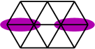
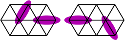
(a)                                    (b)

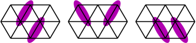
(c)

Figure 7: (Color online) Types of interdimer bond differing in effective interaction due to dimer coordination: (a) “linear”, (b) “semi–linear”, (c) “non–linear”.

The effective interdimer interactions for each type of bond can be deduced in a manner similar to the treatment of the previous section. Considering first the situation for a bond of type (7a) with (os/st) dimers, setting $\langle{\vec{T}}_{i}\cdot{\vec{T}}_{j}\rangle=0$ yields one high–spin and two low–spin terms which contribute

$$H_{1}^{\rm(os,7a)}(0) = -\frac{1}{4}Jr_{1}\Big{(}{\vec{S}}_{i}\cdot{\vec{S}}_{j}+\frac{3}{4}\Big{)},$$

$$H_{2}^{\rm(os,7a)}(0) = \frac{3}{4}Jr_{2}\Big{(}{\vec{S}}_{i}\cdot{\vec{S}}_{j}-\frac{1}{4}\Big{)},$$ (69)

$$H_{3}^{\rm(os,7a)}(0) = \frac{1}{6}J(r_{3}-r_{2})\Big{(}{\vec{S}}_{i}\cdot{\vec{S}}_{j}-\frac{1}{4}\Big{)}.$$

Clearly $H_{1}^{\rm(os,7a)}$ favors FM (high–spin) interdimer spin configurations with coefficient $\frac{1}{4}$, while $H_{2}^{\rm(os,7a)}$ and $H_{3}^{\rm(os,7a)}$ favor AF (low–spin) configurations with coefficient $\frac{3}{8}$ (both at $\eta=0$). Because $r_{1}$ exceeds $r_{2}$ and $r_{3}$ when Hund exchange is finite, one expects a critical value of $\eta$ where FM configurations will be favored. Simple algebraic manipulations using all three terms suggest that this value, which should be relevant for a linear chain of (os/st) dimers, is $\eta_{c}=\frac{1}{8}$. In the limit $\eta\rightarrow 0$, the effective bond Hamiltonian simplifies to

$$H_{\rm eff}^{\rm(os,7a)}(0)=\frac{1}{2}J\left({\vec{S}}_{i}\cdot{\vec{S}}_{j}-\frac{3}{4}\right).$$ (70)

For a bond of type (7a) with (ss/ot) dimers, setting $\langle{\vec{S}}_{i}\cdot{\vec{S}}_{j}\rangle=0$ on the interdimer bond yields

$$H_{1}^{\rm(ss,7a)}(0) = \frac{3}{4}Jr_{1}\left({\vec{T}}_{i}\cdot{\vec{T}}_{j}-\frac{1}{4}\right),$$

$$H_{2}^{\rm(ss,7a)}(0) = -\frac{1}{4}Jr_{2}\left({\vec{T}}_{i}\cdot{\vec{T}}_{j}+\frac{3}{4}\right),$$ (71)

$$H_{3}^{\rm(ss,7a)}(0) = -\frac{1}{6}J(r_{3}-r_{2})\left({\vec{T}}_{i}\times{\vec{T}}_{j}+\frac{1}{4}\right).$$

Here $H_{1}^{\rm(ss,7a)}$ favors AO configurations with coefficient $\frac{3}{8}$, while $H_{2}^{\rm(ss,7a)}$ and $H_{3}^{\rm(ss,7a)}$ both favor FO configurations with coefficient $\frac{1}{4}$ (at $\eta=0$). Over the relevant range of Hund exchange coupling, $0<\eta<1/3$, there is no change in sign and AO configurations are always favored. The effective bond Hamiltonian for $\eta\rightarrow 0$ is

$$H_{\rm eff}^{\rm(ss,7a)}(0)=\frac{1}{2}J\left({\vec{T}}_{i}\cdot{\vec{T}}_{j}-\frac{3}{4}\right).$$ (72)

For bonds of type (7b), when only one electron occupies an active orbital the corresponding decoupled interdimer bond Hamiltonians are, for (os/st) dimers,

$$H_{1}^{\rm(os,1)}(0) = -\frac{1}{4}Jr_{1}\Big{(}{\vec{S}}_{i}\cdot{\vec{S}}_{j}+\frac{3}{4}\Big{)},$$

$$H_{2}^{\rm(os,1)}(0) = \frac{1}{4}Jr_{2}\Big{(}{\vec{S}}_{i}\cdot{\vec{S}}_{j}-\frac{1}{4}\Big{)},$$ (73)

$$H_{3}^{\rm(os,1)}(0) = 0.$$

The final interdimer interaction is obtained by averaging over these expressions and those (IV.1) for two active orbitals per bond, and takes the rather cumbersome form

$$H_{\rm eff}^{\rm(os,7b)}(0) = \frac{1}{12}J\;(r_{3}+5r_{2}-3r_{1})\;{\vec{S}}_{i}\cdot{\vec{S}}_{j}$$ (74)

$$-\frac{1}{48}J\;(9r_{1}+5r_{2}+r_{3}),$$

which reduces in the limit $\eta\rightarrow 0$ to

$$H_{\rm eff}^{\rm(os,7b)}(0)=\frac{1}{4}J\left({\vec{S}}_{i}\cdot{\vec{S}}_{j}-\frac{5}{4}\right).$$ (75)

For (ss/ot) dimers, the situation cannot be formulated analogously, because if only one electron on the bond is active, the orbital state of the other electron has no influence on the hopping process, i.e. ${\vec{T}}_{i}\cdot{\vec{T}}_{j}$ is not a meaningful quantity. The resulting expressions lead then to

$$H_{\rm eff}^{\rm(ss,7b)}(0)\!\! = \!\!\frac{1}{8}J(3r_{1}\!-\!r_{2}){\vec{T}}_{i}\cdot{\vec{T}}_{j}\!-\!\frac{1}{12}J(r_{3}\!-\!r_{2}){\vec{T}}_{i}\!\times\!{\vec{T}}_{j}$$ (76)

$$-\frac{1}{48}J\,(9r_{1}+5r_{2}+r_{3}),$$

which has the $\eta\rightarrow 0$ limit

$$H_{\rm eff}^{\rm(ss,7b)}(0)=\frac{1}{4}J\left({\vec{T}}_{i}\cdot{\vec{T}}_{j}-\frac{5}{4}\right).$$ (77)

Finally, for a bond of type (7c), there is no contribution from interdimer bond states with no electrons in active orbitals, so the above results [(IV.1, IV.1) and (IV.1, 76)] are already sufficient to perform the necessary averaging. With (os/st) dimers

$$H_{\rm eff}^{\rm(os,7c)}(0) = \frac{1}{48}J\,(2r_{3}+13r_{2}-9r_{1})\;{\vec{S}}_{i}\cdot{\vec{S}}_{j}$$ (78)

$$-\frac{1}{192}J\;(27r_{1}+13r_{2}+2r_{3}),$$

which reduces in the limit $\eta\rightarrow 0$ to

$$H_{\rm eff}^{\rm(os,7c)}(0)=\frac{1}{8}J\left({\vec{S}}_{i}\cdot{\vec{S}}_{j}-\frac{7}{4}\right),$$ (79)

while for (ss/ot) dimers,

$$H_{\rm eff}^{\rm(ss,7c)}(0)\!\! = \!\!\frac{1}{16}J(3r_{1}\!-\!r_{2}){\vec{T}}_{i}\cdot{\vec{T}}_{j}\!-\!\frac{1}{24}J(r_{3}\!-\!r_{2}){\vec{T}}_{i}\!\times\!{\vec{T}}_{j}$$ (80)

$$-\frac{1}{192}J\,(27r_{1}+13r_{2}+2r_{3}),$$

which in the $\eta\rightarrow 0$ limit gives

$$H_{\rm eff}^{\rm(ss,7c)}(0)=\frac{1}{8}J\left({\vec{T}}_{i}\cdot{\vec{T}}_{j}-\frac{7}{4}\right).$$ (81)

Table 1: Occurrence probabilities for bonds of each type for four simple periodic dimer coverings of the triangular lattice.

configuration	dimer	bond (7a)	bond (7b)	bond (7c)
Fig. 8(a)	$\frac{1}{6}$	$\frac{1}{6}$	0	$\frac{2}{3}$
Fig. 8(b)	$\frac{1}{6}$	0	$\frac{1}{3}$	$\frac{1}{2}$
Fig. 8(c)	$\frac{1}{6}$	0	$\frac{1}{3}$	$\frac{1}{2}$
Fig. 8(d)	$\frac{1}{6}$	0	$\frac{1}{3}$	$\frac{1}{2}$

These results have clear implications for the nearest–neighbor correlations in an extended system. By inspection, systems composed of either type of dimer would favor AF (spin) and AO interdimer bonds, to the extent allowed by frustration, and “linear” [type (7a)] bonds over “semi–linear” [type (7b)] bonds over “non–linear” [type (7c)] bond types in Fig. 7, to the extent allowed by geometry. Discussion of this type of state requires in principle the consideration of all possible dimer coverings, but will be restricted here to a small number of periodic arrays which illustrate much of the essential physics of extended dimer systems within this model.

We begin by considering the periodic covering of Fig. 8(a), a fully linear conformation (of ground–state degeneracy 12) whose interdimer bond types (Table I) maximize the possible number of bonds of type (7a). The counterpoint shown in Fig. 8(b) consists of pairs of dimer bonds with alternating orientations in two of the three lattice directions, and constitutes the simplest configuration minimizing (to zero) the number of type–(7a) interdimer bonds. The coverings in Figs. 8(c) and (d) have the same property. These configurations exemplify a quite general result, that any dimer covering in which there are no linear configurations [type (7a)] of any pair of dimers will have 1/3 type–(7b) bonds, and thus the remaining 1/2 of the bonds must be of type (7c). The coverings shown in Figs. 8(a) and (b, c, d) represent the limiting cases on numbers of each type of bond, in that any random dimer covering will have values between these. Indeed, it is straightforward to argue that, in changes of position of any set of dimers within a covering, the creation of any two bonds of type (7b) will destroy one of type (7a) and one of type (7c), and conversely.

Having established this effective sum rule, we turn next to the energies of the dimer configurations. First, for both types of dimer [(os/st) and (ss/ot)], all states with equal numbers of each bond type are degenerate, subject to equal solutions of the frustration problem. Next, if frustration is neglected, it is clear from Eqs. (70,72), (75,77), and (79,81), that the AF and AO energy values for the three bond types (obtained by substituting $-\frac{1}{4}$ for ${\vec{S}}_{i}\cdot{\vec{S}}_{j}$ and ${\vec{T}}_{i}\cdot{\vec{T}}_{j}$) are respectively $-\frac{1}{2}J$, $-\frac{3}{8}J$ and $-\frac{1}{4}J$, which, when taken together with the sum rule, suggest a very large degeneracy of dimer covering energies.

  

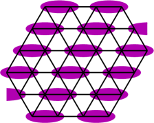
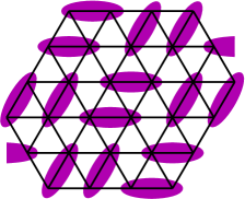
(a)                               (b)

  

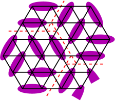
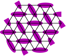
(c)                               (d)

Figure 8: (Color online) Periodic dimer coverings on the triangular lattice, each representative of a class of coverings: (a) linear; (b) plaquette; (c) 12–site unit cell; (d) “zig–zag”.

Returning to the question of frustration, a covering of minimal energy is one which both minimizes the number of FM or FO bonds, and ensures that they fall on bonds of type (7c); both criteria are equally important. For the dimer covering (8a), with maximal aligned bonds, it is possible by using the spin (for (os/st) dimers) or orbital (for (ss/ot) dimers) configuration represented by the arrows in Fig. 9(a) to make the number of frustrated (FM/FO) interdimer bonds equal to 1/6 of the total. Bearing in mind that the 1/6 of bonds covered by dimers are also FM/FO, and that at least 1/3 of bonds on the triangular lattice must be frustrated for collinear spins, this number is an absolute minimum. [Here we do not consider the possibility of non–collinear order of the non–singlet degree of freedom.] Further, for this configuration one observes that all of the FM/FO bonds already fall on bonds of type (7c), providing an optimal case with energy

$$E_{\rm dim}(0) = -J\left(\frac{1}{6}+\frac{1}{6}\cdot\frac{1}{2}+\frac{1}{2}\cdot\frac{1}{4}+\frac{1}{6}\cdot\frac{3}{16}\right)$$ (82)

$$= -\frac{13}{32}J$$

at $\eta=0$. This value constitutes a basic bound which demonstrates that a simple, static dimer covering has lower energy than any long–range–ordered spin or orbital state discussed in Sec. III in this limit ($\alpha=0$) of the model.

  

(a)                               (b)

Figure 9: (Color online) Spin or orbital configurations (black arrows) within (a) linear and (b) zig–zag orbital– or spin–singlet dimer coverings of the triangular lattice. The number of frustrated interdimer bonds is reduced to 1/6 of the total, and all are of type (7c). This figure emphasizes that for the spin–orbital model, dimer singlet formation does not exhaust the available degrees of freedom.

It remains to establish the degeneracy of the ground–state manifold of such coverings, and we provide only a qualitative discussion using further examples. If alternate four–site (dimer pair) clusters in Fig. 8(a) are rotated to give the covering of Fig. 8(b), the minimal frustration is spoiled: by analogy with Fig. 9, it is easy to show that, if only 1/6 of the bonds are to be frustrated, then they are of type (7b), and otherwise 1/3 of the bonds are frustrated if all are to be of type (7c). On the periodic 12–site cluster [Fig. 8(c)], one may place three four–site clusters in each of the possible orientations, which as above removes all bonds of type (7a) and maximizes those of type (7b). Within this cluster it is possible to have only four frustrated interdimer bonds out of 18, while between the clusters there is again an arrangement of the spin or orbital arrows (cf. Fig. 9) with only six FM or FO bonds out of 24, for a net total of 1/6 frustrated interdimer bonds, of which half are of type (7b). The covering of Fig. 8(d) represents an extension of the procedure of enlarging unit cells and removing four–site plaquettes, which demonstrates that it remains possible in the limit of no type–(7a) bonds to reduce frustration to 1/6 of the bonds, and to bonds of type (7c) [Fig. 9(b)], whence the energy of the covering is again $E_{\rm dim}(0)=-\frac{13}{32}$ (82). Thus it is safe to conclude that, for the static–dimer problem, the ground–state manifold for $\alpha=0$ consists of a significant number of degenerate coverings. We do not pursue these considerations further because of degeneracy lifting by dimer resonance processes, and because the energetic differences between static dimer configurations are likely to be dwarfed by the contributions from dimer resonance, the topic to which we turn in Sec. V.

IV.2 Direct exchange model

The very strong preference for bond spin singlets (the factor of 4 in Eq. (23)] suggests that dimer states will also be competitive in this limit, even though only 1/6 of the bonds may redeem an energy of $-J$. Following the considerations and terminology of the previous subsection, we note (i) that $\langle{\vec{S}}_{i}\cdot{\vec{S}}_{j}\rangle=0$ on interdimer bonds and (ii) that in this case, interdimer bonds have energy $-\frac{1}{4}J$ at $\eta=0$ for types (7a) and (7b), and $0$ for type (7c). Because any state with a maximal number (1/6) of type–(7a) bonds must have only bonds of type (7c) for the other 2/3 [states (8a)], such a state is manifestly less favorable at $\alpha=1$ than those of type (8b)–(8d), where there are no aligned pairs of dimers. In this latter case, the full calculation gives

$$E_{\rm dim}(1)=-\frac{1}{144}J(9r_{1}+19r_{2}+8r_{3}),$$ (83)

and $E_{\rm dim}(1)=-\frac{1}{4}J$ for $\eta=0$. This energy does now exceed that available from the formation of Heisenberg spin chains in one of the three lattice directions (Sec. III.3), which gave the value $E_{\rm 1DAF}(1)=-0.231J$.

At the level of these calculations, the manifold of degenerate states with this energy is very large, and its counting is a problem which will not be undertaken here. We will show in Sec. V that, precisely in this limit, no dimer resonance processes occur and the static dimer coverings do already constitute a basis for the description of the ground state. The question of fluctuations leading to the selection of a particular linear combination of these states which is of lowest energy, i.e. of a type of order–by–disorder mechanism, is addressed in Ref. Jac07, .

At finite values of the Hund exchange, this type of state will come into competition with the simple avoided–blocking states which gain, with a FM spin state, an energy

$$E_{\rm FM}(1)=-\frac{1}{6}Jr_{1},$$ (84)

as 2/3 of the bonds contribute with an energy of $-\frac{1}{4}Jr_{1}$. The critical value of $\eta$ required to drive the transition from the low–spin dimerized state to the FM state is found to be

$$\eta_{c}=0.1589.$$ (85)

IV.3 Mixed model

Because both of the endpoints, $\alpha=0$ and $\alpha=1$, favor dimerized states over states of long–ranged order, it is natural to expect that a dimer state will provide a lower energy also at $\alpha=0.5$. However, we remind the reader that there are no intermediate dimer bases, and caution there is no strong reason to expect one or other of the limiting dimer states to be favored close to $\alpha=0.5$. By inspection, the energy of an $\alpha>0$ state can be obtained by direct addition of the diagonal interdimer bond contributions in an (ss/ot) or (os/st) dimer state, which is established by pure off–diagonal hopping, because no site occupancies arise which allow mixed processes. For the same reason, no interdimer terms impede a calculation of the energy of an $\alpha<1$ state by summing the off–diagonal interdimer bond contributions in a spin–singlet dimer state stabilized by purely diagonal processes. We will not analyze the static dimer solutions for the intermediate regime in great detail, and provide only a crude estimate of the $\alpha=0.5$ energy by averaging over both results at the limits of their applicability. We will make no attempt here to exclude other forms of disordered state at $\alpha=0.5$, and return to this question in Sec. V.

Table 2: Additional interdimer bond energies at $\alpha=0.5$ due respectively to (i) diagonal hopping occurring in a state (designated by $\alpha=0$) stabilized by off–diagonal processes and (ii) off–diagonal hopping in a state ($\alpha=1$) stabilized by diagonal processes.

bond	(7a)	(7b)	(7c)
$\alpha=0$, (os/st), AF	0	$-\frac{1}{16}(r_{1}+r_{2})$	$-\frac{1}{8}(r_{1}+r_{2})$
$\alpha=0$, (os/st), FM	0	$-\frac{1}{8}r_{1}$	$-\frac{1}{4}r_{1}$
$\alpha=0$, (ss/ot), AO	0	$-\frac{1}{32}(3r_{1}+r_{2})$	$-\frac{1}{16}(3r_{1}+r_{2})$
$\alpha=0$, (ss/ot), FO	0	$-\frac{1}{32}(3r_{1}+r_{2})$	$-\frac{1}{16}(3r_{1}+r_{2})$
$\alpha=1$, $\parallel$ dimers	0	$-\frac{1}{16}(3r_{1}+r_{2})$	$-\frac{1}{8}(3r_{1}+r_{2})$
$\alpha=1$, non–$\parallel$ dimers	0	$-\frac{1}{16}(3r_{1}+r_{2})$	$-\frac{1}{12}(2r_{2}+r_{3})$

For each type of bond it is straightforward to compute the energy gained from interdimer hopping processes of the type not constituting the dimer state, and the results are shown in Table II. The first four lines give the energies per bond from diagonal hopping processes occurring on the bonds of the different $\alpha=0$ dimer states, and conversely for the final two lines. It is clear that the occupations of type (7a) bonds preclude any hopping of the opposite type. For $\alpha=0$ dimer configurations, the interdimer diagonal hopping on (7b) bonds is always of avoided–blocking type, while on (7c) bonds a blocking can occur, and like the other terms is evaluated using $\langle{\vec{S}}_{i}\cdot{\vec{S}}_{j}\rangle$. For $\alpha=1$, off–diagonal hopping on the interdimer bonds is evaluated with $\langle{\vec{S}}_{i}\cdot{\vec{S}}_{j}\rangle=0$ between the spin singlets: all processes on (7b) bonds are those for one active orbital; complications arise only for (7c) bonds, where an interdimer bond between parallel dimers has two active AO orbitals, while one between dimers which are not parallel has two active FO orbitals.

At $\alpha=0.5$, the energy of an (os/st) or (ss/ot) dimer state augmented by diagonal hopping processes is minimized by states (8a) and (8d): the interdimer bond contributions of all coverings in Fig. 8 are equal, despite the different type counts, so only the $\alpha=0$ energy is decisive. At $\eta=0$,

$$E_{o}^{(\ref{pdc}a)}(0.5) = -\frac{1}{2}\left(\frac{13}{32}+\frac{2}{3}\!\cdot\!\frac{1}{4}\right)J\;=\;-\frac{55}{192}\,J,\;\;\;\;\;\;$$ (86)

$$E_{o}^{(\ref{pdc}d)}(0.5) = -\frac{1}{2}\left(\frac{13}{32}+\frac{1}{3}\!\cdot\!\frac{1}{8}+\frac{1}{2}\!\cdot\!\frac{1}{4}\right)J$$ (87)

$$= -\frac{55}{192}\,J.$$

The energy of a spin–singlet dimer state augmented by off–diagonal hopping is minimal in states (8b) and, curiously, (8a): although the latter has explicitly a worse ground–state energy than the other states shown, the effect of the additional hopping is strong, not least because all interdimer type–(8c) bonds are between parallel dimers. Thus at $\eta=0$,

$$E_{d}^{(\ref{pdc}a)}(0.5) = -\frac{1}{2}\left(\frac{5}{24}+\frac{1}{2}\cdot\frac{2}{3}\right)J\;\;=\;\;-\frac{13}{48}J,$$

$$E_{d}^{(\ref{pdc}b)}(0.5) = -\frac{1}{2}\left(\frac{1}{4}+\frac{1}{3}\cdot\frac{1}{4}+\frac{1}{2}\cdot\frac{2}{3}\cdot\frac{1}{2}+\frac{1}{2}\cdot\frac{1}{3}\cdot\frac{1}{4}\right)J$$ (88)

$$= -\frac{13}{48}J.$$

Despite the fact that these are two completely different expansions, it is worth noting that the two sets of numbers are rather similar, which occurs because the significantly inferior energy of the $\alpha=1$ ground state is compensated by the significantly greater interdimer bond energies available from off–diagonal hopping processes. However, this result also implies that no special combinations of diagonal and off–diagonal dimers can be expected to yield additional interdimer energies beyond this value.

Taking the covering (8a) as representative of the lowest available energy, but bearing in mind that many other states lie very close to this value, an average over the two approaches yields

$$E_{\rm dim}^{(\ref{pdc}a)}(0.5)=-\frac{107}{384}J$$ (89)

at $\eta=0$. This number is no longer lower than the value obtained in Sec. IIID for fully ordered states gaining energy from mixed processes, raising the possibility that non–dimer–based phases may be competitive in the intermediate regime, where neither of the limiting types of dimer state alone is expected to be particularly suitable. However, we will not investigate this question more systematically here, and caution that the approximations made both in Sec. IIID and here make it difficult to draw a definitive conclusion.

IV.4 Summary

The results of this section make it clear that static dimer states, while showing the same energetic trend, are considerably more favorable than any long–range–ordered states (Sec. III) over most of the phase diagram. As a function of $\alpha$, the dimer energy increases monotonically from $-\frac{13}{32}J$ to $-\frac{1}{4}J$, and both end–point values also lie below the results obtained for quasi–1D spin–disordered states in Sec. III. We stress that the results of this section are provisional in the sense that we have not performed a systematic exploration of all possible dimer coverings, but rather have focused on a small number of examples illustrative of the limiting cases in terms of interdimer bond types. More importantly, we have considered only static dimer coverings with effective interdimer interactions: the kinetic energy contributions due to dimer resonance processes for all values of $\alpha<1$ are missing in this type of calculation. For this reason, we have also refrained from investigating higher–order processes, which may select particular dimer states from a manifold of static coverings degenerate at the level of the current considerations. Gaining some insight into the magnitude and effects of resonance contributions is the subject of the following section.

V Exact diagonalization

V.1 Clusters and correlation functions

In this Section we present results obtained for small systems by full exact diagonalization (ED). Because each site has two spin and three orbital states, the dimension of the Hilbert space increases with cluster size as $6^{N}$, where $N$ is the number of sites. As a consequence, we focus here only on systems with $N=$ 2, 3, and 4 sites: all three clusters can be considered as two–, three– or four–site segments of an extended triangular lattice, connected with periodic boundary conditions. For the single bond and triangle this only alters the bond energies by a factor of two, a rescaling not performed here, but for the four–site system it is easy to see that the intercluster bonds ensure that the system connectivity is tetrahedral. We will also compare some of the single–bond and tetrahedron results with those for a four–site chain. Other accessible cluster sizes ($N=$ 5 and 6) yield awkward shapes which disguise the intrinsic system properties. Indeed we will emphasize throughout this Section those features of our very small clusters which can be taken to be generic, and those which are shape–specific.

Given the clear tendency to dimerization illustrated in Secs. III and IV, it is to be expected that spin correlation lengths in all regimes of $\alpha$ are very small. To the extent that the behavior of the model for any parameter set is driven by local physics, the cluster results should be highly instructive for such trends as dimer formation, relative roles of diagonal and off–diagonal hopping, dimer resonance processes, lifting of degeneracies both in the orbital sector and between states of (os/st) and (ss/ot) dimers, and the importance of joint spin–orbital correlations. However, generic features of extended systems which cannot be accessed in small clusters are those concerning questions of high system degeneracy and subtle selection effects favoring specific states.

We will compute and discuss the cluster energies, degeneracies, site occupations, bond hopping probabilities in diagonal and off–diagonal channels (discussed in Sec. VC), and the spin, orbital, and spin–orbital (four–operator) correlation functions. All of these quantities will be calculated for representative values of $\alpha$ and $\eta$ covering the full phase diagram, and each contains important information of direct relevance to the local physics properties listed in the previous paragraph. Although the systems we study are perforce rather small, we will show that one may recognize in them a number of general trends valid also in the thermodynamic limit.

We introduce here the three correlation functions, which for a bond $\langle ij\rangle$ oriented along axis $\gamma$ are given respectively by

$$S_{ij}\! \equiv \frac{1}{d}\;\sum_{n}\big{\langle}n\big{|}{\vec{S}}_{i}\cdot{\vec{S}}_{j}\big{|}n\big{\rangle},$$ (90)

$$T_{ij}\! \equiv \frac{1}{d}\;\sum_{n}\big{\langle}n\big{|}{\vec{T}}_{i\gamma}\cdot{\vec{T}}_{j\gamma}\big{|}n\big{\rangle},$$ (91)

$$C_{ij}\! \equiv \!\frac{1}{d}\;\sum_{n}\big{\langle}n\big{|}({\vec{S}}_{i}\!\cdot\!{\vec{S}}_{j})({\vec{T}}_{i\gamma}\!\cdot\!{\vec{T}}_{j\gamma})\big{|}n\big{\rangle}$$ (92)

$$- \!\frac{1}{d^{2}}\sum_{n}\big{\langle}n\big{|}{\vec{S}}_{i}\!\cdot\!{\vec{S}}_{j}\big{|}n\big{\rangle}\sum_{m}\big{\langle}m\big{|}{\vec{T}}_{i\gamma}\!\cdot\!{\vec{T}}_{j\gamma}\big{|}m\big{\rangle},$$

where $d$ is the degeneracy of the ground state. The definitions of the spin ($S_{ij}$) and orbital ($T_{ij}$) correlation functions are standard, and we have included explicitly all of the quantum states $\{|n\rangle\}$ which belong to the ground–state manifold. The correlation function $C_{ij}$ (92) contains information about spin–orbital entanglement, as defined in Sec. I: it represents the difference between the average over the complete spin–orbital operators and the product of the averages over the spin and orbital parts taken separately. It is formulated in such a way that $C_{ij}=0$ means the mean–field decoupling of spin and orbital operators on every bonds is exact, and both subsystems may be treated independently from each other. Such exact factorizability is foundOle06 in the high–spin states at large $\eta$; its breaking, and hence the need to handle coupled spin and orbital correlations in a significantly more sophisticated manner, is what is meant by “entanglement” in this context.

V.2 Single bond

We consider first a single bond oriented along the $c$–axis (Fig. 10). In the superexchange limit the active orbitals are $a$ and $b$, while for direct exchange only the $c$ orbitals contribute in Eq. (9). As discussed in Sec. IV.1, a single bond gives energy $-J$ in the superexchange model ($\alpha=0$) [Fig. 10(a)], where the ground state has degeneracy $d=6$ at $\eta=0$, from the two triply degenerate wave functions (ss/ot) and (os/st). At finite $\eta$, the latter is favored as it permits a greater energy gain from excitations to the lowest triplet state in the $d^{2}$ configuration [Eqs. (17) and (18)].

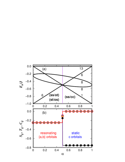
Figure 10: (Color online) Evolution of the properties of a single bond $\gamma\equiv c$ as a function of $\alpha$ at $\eta=0$: (a) energy spectrum (solid lines) with degeneracies as shown; (b) spin ($S_{ij}$, filled circles), orbital ($T_{ij}$, empty circles), and spin–orbital ($C_{ij}$, $\times$) correlations: $S_{ij}=T_{ij}=C_{ij}=-0.25$ for $\alpha<0.5$, while $T_{ij}=C_{ij}=0$ for $\alpha>0.5$. The ground–state energy $E_{0}$ is $-J$ for both the superexchange ($\alpha=0$) and direct–exchange ($\alpha=1$) limits, and its increase between these is a result of the scaling convention. The transition between the two regimes occurs by a level crossing at $\alpha=0.5$. For $\alpha<0.5$, the two types of dimer wave function [(ss/ot) and (os/st)] are degenerate ($d=6$) for resonating orbital configurations $\{ab\}$, while at $\alpha>0.5$, the nondegenerate spin singlet is supported by occupation of $c$ orbitals at both sites [(ss/cc)].

Although orbital fluctuations which appear in the mixed exchange terms in Eq. (24) may in principle contribute at $\alpha>0$, one finds that the wave function remains precisely that for $\alpha=0$, i.e. (ss/ot) degenerate with (os/st), all the way to $\alpha=0.5$. Thus for the parameter choice specified in Sec. II, the ground–state energy increases to a maximum of $E_{0}=-0.5J$ here [Fig. 10(a)]. The degeneracy $d=6$ is retained throughout the regime $\alpha<0.5$, and only at $\alpha=0.5$ do several additional states join the manifold, causing the degeneracy to increase to $d=15$. For the entire regime $\alpha\in(0.5,1]$, the ground state is a static orbital configuration with $c$ orbitals occupied at both sites to support the spin singlet, and $d=1$. The evolution of the spectrum with $\alpha$ demonstrates not only that superexchange and direct exchange are physically distinct, unable to contribute at the same time, but that the two limiting wave functions are extremely robust, their stability quenching all mixed fluctuations for a single bond. In this situation it is not the ground–state energy but the higher first excitation energy which reveals the additional quantum mechanical degrees of freedom active at $\alpha=0$ compared to $\alpha=1$ [Fig. 10(a)].

The spin, orbital, and composite spin–orbital correlation functions defined in Eqs. (90)–(92) give more insight into the nature of the single–bond correlations. The degeneracy of wavefunctions (ss/ot) and (os/st) for $0\leq\alpha<0.5$ leads to equal spin and orbital correlation functions, as shown in Fig. 10(b), and averaging over the different states gives $S_{ij}=T_{ij}=-\frac{1}{4}$. As a singlet for one quantity is matched by a triplet for the other, the two sectors are strongly correlated, and indeed $C_{ij}=-\frac{1}{4}$, indicating an entangled ground state. However, a considerably more detailed analysis is possible. Each of the six individual states $\{|n\rangle\}$ within the ground manifold has the expectation value $\big{\langle}n\big{|}({\vec{S}}_{i}\!\cdot\!{\vec{S}}_{j})({\vec{T}}_{i\gamma}\!\cdot\!{\vec{T}}_{j\gamma})\big{|}n\big{\rangle}=-\frac{3}{16}$, which we assert is the minimum possible when the spin and pseudospin are the quantum numbers of only two electrons. It is clear that if the operator in $C_{ij}$ is evaluated for any one of these states alone, the result is zero. Entanglement arises mathematically because of the product of averages in the second term of Eq. (92), and physically because the ground state is a resonant superposition of a number of degenerate states. We emphasize that the resulting value, $C_{ij}=-\frac{1}{4}$, is the minimum obtainable in this type of model, reflecting the maximum possible entanglement. We will show in Sec. VE that this value is also reproduced for the Hamiltonian of Eq. (9) on a linear four–site cluster, whose geometry ensures that the system is at the SU(4) point of the 1D SU(2)$\otimes$SU(2) model.Ole06

By contrast, for $\alpha>0.5$ those states favored by superexchange become excited, and the spin–singlet ground state has $S_{ij}=-\frac{3}{4}$. The orbital configuration is characterized by $\langle n_{ic}n_{jc}\rangle=1$, a rigid order which quenches all orbital fluctuations (indeed, the orbital pseudospin variables ${\vec{T}}_{i\gamma}$ are zero). Thus the spin and orbital parts are trivially decoupled, giving $C_{ij}=0$. Finally, at the transition point $\alpha=0.5$, averaging over all 15 degenerate states yields $S_{ij}=-0.15$, $T_{ij}=-0.10$, and $C_{ij}=-0.09$. In summary, the very strong tendency to dimer formation in the two limits $\alpha=0$ and $\alpha=1$ precludes any contribution from mixed terms on a single bond, leading to a very simple interpretation of the ground–state properties for all parameters.

V.3 Triangular cluster

We turn next to the triangle, which has one bond in each of the lattice directions $a$, $b$, and $c$. Unlike the case of the single bond, here the spin–orbital interactions are strongly frustrated, in a manner deeper than and qualitatively different from the Heisenberg spin Hamiltonian. Not only can interactions on all three bonds not be satisfied at the same time, but also the actual form of these interactions changes as a function of the occupied orbitals. The triangle is sufficient to prove (numerically and analytically) the inequivalence in general of the original model and the model after local transformation, for frustration reasons discussed in Sec. II.2.

We begin with the observation that the results to follow are interpreted most directly in terms of resonant dimer states on the triangle. This fact is potentially surprising, given that the number of sites is odd and dimer formation must always exclude one of them, but emphasizes the strong tendencies to dimer formation in all parameter regimes of the model. For their interpretation we use a VB ansatz where it is assumed that one bond is occupied by an optimal dimer state, minimizing its energy, and the final state of the system is determined by the contributions of the other two bonds. This ansatz is perforce only static, and breaks the symmetry at a crude level, but enables one to understand clearly the effects of the resonance processes captured by the numerical studies in restoring symmetries and lowering the total energy.

Considering first the VB ansatz for the superexchange model, the energy $-J$ may be gained only on a single bond, in one of two ways. For the bond spin state to be a singlet ($S=0$, (ss/ot) wave function), two different active orbitals are occupied at both sites in one of the orbital triplet states. The other two bonds lower the total energy when the third site has an electron of the third orbital color, each gaining an energy of $-0.25J$ due to the orbital interactions in Eq. (10). The energy of the triangle is then $E_{\rm VB}(0)=-0.5J$ per bond, and the cluster has a low–spin ($S=\frac{1}{2}$) ground state with degeneracy $d=6$ from the combination of the orbital triplet and the spin state of the third electron. We stress that the location ($a$, $b$, or $c$ bond) of the spin singlet does not contribute to the degeneracy because the three VB states are mixed within the ground state by the contributing off–dimer hopping processes. The same considerations applied to an (os/st) dimer on one of the bonds of the triangle shows that there is no color and spin state of the third electron which allows both non–dimer bonds to gain the energy $-0.25J$ simultaneously, so the cluster has a higher energy of $-\frac{5}{12}J$ per bond. Thus the VB ansatz illustrates a lifting of the degeneracy between the two types singlet state, the physical origin of which lies in the permitted off–dimer fluctuation processes, and this will be borne out in the calculations below. However, the net spin state of the cluster has little effect on the estimated energy of the (os/st) case, and its high–spin version ($S=\frac{3}{2}$) will be a strong candidate for the ground state at higher values of $\eta$. In the direct–exchange limit ($\alpha=1$), the VB ansatz for spin singlets again returns an energy $E_{\rm VB}(1)=-\frac{5}{12}J$, also because only one non–dimer bond can contribute. Here the off–dimer processes are restricted to the third electron, which has arbitrary color and spin, and cannot mix the three VB states, whence the degeneracy is $d=12$.

With this framework in mind, we turn to a description of the numerical calculations at all values of $\alpha$, beginning with the most important results: at $\alpha=0$ the degeneracy is $d=6$, and hence VB resonance is confirmed, yielding an energy very much lower than the static estimate, at $E_{0}=-0.75J$ per bond [Fig. 11(a)]. Thus strong orbital dynamics and positional resonance effects operate in the ground–state manifold. These break the (ss/ot)/(os/st) symmetry, but act to restore other symmetries broken in the VB ansatz. At $\alpha=1$, the energy and degeneracy from the VB ansatz are exact, showing that the orbital sector is classical andintroduces no resonance effects.

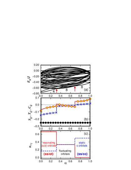
Figure 11: (Color online) (a) Energy spectrum per bond for a triangular cluster as a function of $\alpha$ for $\eta=0$. Ground–state degeneracies are as indicated, with $d=6$ at $\alpha=0$ and $d=12$ at $\alpha=1$. The arrows mark two transitions in the nature of the (low–spin) ground state, which are further characterized in panels (b) and (c). (b) Spin ($S_{ij}$, filled circles), orbital ($T_{ij}$, empty circles), and spin–orbital ($C_{ij}$, $\times$) correlation functions on the $c$ bond. (c) Average electron densities in the $t_{2g}$ orbitals at site 1 [Figs. 2(b,c)], showing $n_{1b}$ (solid line) and $n_{1a}=n_{1c}$ (dashed). The orbital labels are shown for a $c$ bond. All three panels show clearly a superexchange regime for $\alpha<0.32$, a direct–exchange regime for $\alpha>0.69$, and an intermediate regime ($0.32<\alpha<0.69$). A full description is presented in the text.

Figure 11(a) shows the complete spectrum of the triangular cluster for all ratios of superexchange to direct exchange, and in the absence of Hund coupling. Frustration of spin–orbital interactions is manifest in rather dense energy spectra away from the symmetric points, and in a ground–state energy per bond significantly higher than the minimal value $-J$. At $\alpha=0$ the spectrum is rather broad, with a significant number of states of relatively low degeneracy due to the strong fluctuations and consequent mixing of VB states in this regime. However, even in this case the ground state is well separated from the first excited state. As emphasized above, the ground–state energy, $E_{0}(0)=-0.75J$, is quite remarkable, demonstrating a very strong energy gain from dimer resonance processes. By contrast, the value $E_{0}(1)=-\frac{5}{12}J$ per bond found at $\alpha=1$ is exactly equal to that deduced from the VB ansatz, demonstrating that this wave function is exact. Here the excited states have high degeneracies, mostly of orbital origin, and thus the spectrum shows wide gaps between these manifolds of states; this effect is more clearly visible in Fig. 12(c). The degeneracies shown in Fig. 11(a) are discussed below. In the intermediate regime, many of the degeneracies at the end–points are lifted, leading to a very dense spectrum. The two transitions at $\alpha=0.32$ and $\alpha=0.69$ appear as clear level–crossings: the intermediate ground state is a highly excited state in both of the limits ($\alpha=0,1$), reinforcing the physical picture of a very different type of wave function dominated by orbital fluctuations and, as we discuss next, with little overt dimer character.

The correlation functions for any one bond of the triangle are shown in Fig. 11(a). That $S_{ij}$ is constant for all $\alpha$ can be understood in the dimer ansatz by averaging over the three configurations with one (ss/ot) or (ss) bond and one ’decoupled’ spin on the third site, which gives $S_{ij}=-\frac{1}{4}$ everywhere. The orbital and spin–orbital correlation functions show a continuous evolution accompanied by discontinuous changes at two transitions, where the nature of the ground state is altered. The orbital correlation function $T_{ij}=-\frac{1}{12}$ at $\alpha=0$ may be understood as an average over the orbital triplet ($+\frac{1}{4}$) and the two non–dimer bonds (each $-\frac{1}{4}$). When $\alpha$ increases, this value is weakened by orbital fluctuations, and undergoes a transition at $\alpha=0.32$ to a regime where orbital fluctuations dominate, and $T_{ij}$ is close to zero. Above $\alpha=0.69$, $T_{ij}$ becomes positive, and approaches $+\frac{1}{12}$ as $\alpha\rightarrow 1$, indicating that the wave function changes to the static–dimer limit. While ${\vec{T}}_{ic}$ vanishes on the $c$ bond here, the cluster average has a finite value due to the contribution $T_{ij}=\frac{1}{4}$ from the active non–singlet bond.

The spin–orbital correlation function $C_{ij}$ also marks clearly the three different regimes of $\alpha$. When $\alpha<0.32$, $C_{ij}$ has a significant negative value [Fig. 11(b)] whose primary contributions are given by the four–operator component $\langle({\vec{S}}_{i}\!\cdot\!{\vec{S}}_{j})({\vec{T}}_{i\gamma}\!\cdot\!{\vec{T}}_{j\gamma})\rangle$. By contrast, $C_{ij}$ is close to zero in the intermediate regime, increasing again to positive values for $\alpha>0.69$. For all $\alpha>0.32$, $C_{ij}$ can be shown to be dominated by the term $-S_{ij}T_{ij}$ in Eq. (92), while the four–operator contribution is small, and vanishes as $\alpha\rightarrow 1$. Thus entanglement, defined as the lack of factorizability of the spin and orbital sectors, can be finite even for vanishing joint spin–orbital dynamics.

Further valuable information is contained in the orbital occupancies at individual sites [Fig. 11(b)], which show clearly the three different regimes. Although there is always on average one electron of each orbital color on the cluster, these are not equally distributed, as each site participates only in two bonds and the symmetry is broken. A representative site, labelled $1$ in Figs. 2(b,c)] has only $a$ and $c$ bonds, and hence the electron density in the $b$ orbital is expected to differ from the other two. The values $n_{b}=2/3$ and $n_{a}=n_{c}=1/6$ found in the regime $\alpha<0.32$ is understood readily as following from a 1/3 average occupation of $(ab)$ and $(bc)$ orbital triplet states on the $c$ and $a$ bonds, respectively, and of an $(ac)$ orbital triplet state on the $b$ bond, which ensures that the electron at site $1$ is in orbital $b$ [Fig. 2(b)]. By contrast, in the regime $\alpha>0.69$, only the two static orbital configurations $(cc)$ and $(bb)$ on the $c$ and $b$ bonds contribute, and $n_{a}=n_{c}=\frac{1}{2}$, while $n_{b}=0$; when the system is in the third possible spin–singlet state, with a $(bb)$ orbital state on the $b$ bond, the third electron is either $a$ or $c$. Between these two regimes ($0.32<\alpha<0.69$) is an extended phase with equal average occupancy of all three orbitals at each site, a potentially surprising result given the broken site symmetry of the cluster. While this may be interpreted as a restoration of the symmetry of the orbital sector by strong orbital fluctuations, including those due to terms in $H_{m}$ (24), it does not imply a higher symmetry of the strongly frustrated interactions at $\alpha=0.5$.

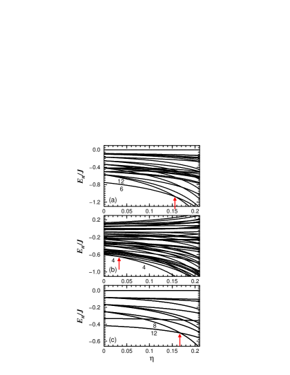
Figure 12: (Color online) Energy spectra for a triangular cluster as a function of Hund exchange $\eta$. Energies are quoted per bond, and shown for: (a) $\alpha=0$, (b) $\alpha=0.5$, and (c) $\alpha=1$. The arrows indicate transitions at $\eta_{c}$ from the low–spin ($S=1/2$) to the high–spin ($S=3/2$) ground state. The numbers in all panels give degeneracies for the two lowest states for $\eta<\eta_{c}$ and $\eta>\eta_{c}$, respectively.

The spectra as a function of Hund coupling $\eta$ are shown in Fig. 12 for the $\alpha=0$ and $\alpha=1$ limits, and at $\alpha=0.5$ to represent the intermediate regime. The lifting of degeneracies as a function of $\eta$ is a generic feature. States of higher spin are identifiable by their stronger dependence on $\eta$, and in all three panels a transition is visible from a low–spin to a high–spin state. At $\alpha=0$ [Fig. 12(a)], the large low–$\eta$ gap to the next excited state results in the transition occurring at the rather high value of $\eta_{c}=0.158$. This can be taken as a further indication of the exceptional stability of the resonance–stabilized ground state in the low–spin sector. The degeneracy $d=12$ of the high–spin state is discussed below.

The transition to the high–spin state at $\alpha=1$ also occurs at a high critical value, $\eta_{c}=0.169$ [Fig. 12(a)], due in this case quite simply to the lack of competition for the strong singlet states on individual bonds. Only in the intermediate regime, $0.32<\alpha<0.69$, where we have shown already that the orbital state is quite different from that in either limit [Fig. 11], is the transition to the high–spin state much more sensitive to $\eta$. The orbital fluctuations in this phase occur both in the low–spin and the high–spin channel, making these very similar in energy, and the transition occurs for $\alpha=0.5$ at only $\eta_{c}=0.033$ [Fig. 12(b)]. As expected from the $\alpha=0$ limit, where fluctuations are also strong, the characteristic features of this energy spectrum are low degeneracy and a semicontinuous nature. The location of the high–spin transition as a function of $\alpha$ may be used to draw a phase diagram for the triangular cluster, which has the rather symmetric form shown in Fig. 13.

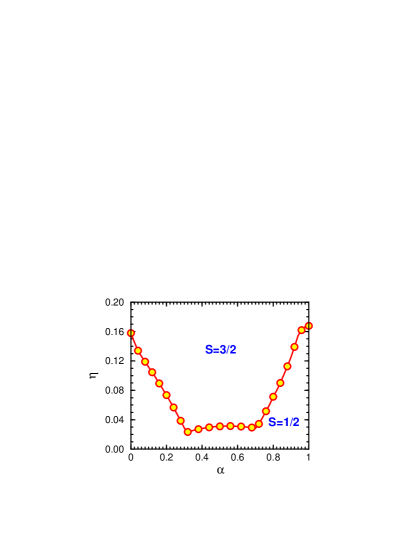
Figure 13: (Color online) Phase diagram of the triangular cluster in the plane $(\alpha,\eta)$. The spin states below and above the transition line $\eta_{c}(\alpha)$ are respectively spin doublet ($S=1/2$) and spin quartet ($S=3/2$).

Yet more information complementary to that in the energy spectra and correlation functions can be obtained by considering the average “occupation correlations” for a bond $\langle ij\rangle\parallel\gamma$,

$$P = \langle n_{i\gamma}n_{j\gamma}\rangle,$$ (93)

$$Q = \langle n_{i\gamma}(1-n_{j\gamma})\rangle+\langle(1-n_{i\gamma})n_{j\gamma}\rangle,$$ (94)

$$R = \langle(1-n_{i\gamma})(1-n_{j\gamma})\rangle.$$ (95)

These probabilities ($P+Q+R=1$) reflect directly the nature of the resonance processes contributing to the energy of the cluster states, in that they show the relative importance of diagonal and off–diagonal hopping in the ground states, and the evolution of these contributions with $\alpha$ and $\eta$. We do not present these quantities in detail here, but only summarize the overall picture of the ground state whose understanding they help elucidate.

For this summary we return to the VB framework, which accounts for many of the basic properties illustrated in the numerical results presented above. Considering first the low–spin states ($\eta=0$), at $\alpha=0$ the ground state is given by one (ss/ot) dimer resonating around the three bonds of the cluster; the third site has the third color, its hopping gives a large value of $Q=1/3$ ($R=2/3$ from the pure superexchange channel) and its spin an addition twofold degeneracy ($d=3\times 2=6$); the orbital occupation of the (ss/ot) dimer is responsible for the net 1/6:1/6:2/3 occupation distribution. When $\alpha>0$ the state remains essentially one with a resonating spin singlet, large $Q$ and dominant $R$, but the orbital triplet degeneracy is lifted to $2+1$ and the ground–state degeneracy to $d=2\times 2$. All quantities, including $P$, $Q$, and $R$, undergo discontinuous changes at $\alpha\simeq 0.32$, and in this regime there is no longer strong evidence for an interpretation in terms of resonating spin singlets: large $Q\simeq 2/3$ and the equal site occupations suggest the dominance of mixed hopping processes which are not consistent with either mechanism of singlet formation. The retention of fourfold degeneracy across this transition is largely accidental, and stems from twofold spin and orbital contributions. Only for $\alpha>0.69$ is a spin–singlet description once again valid: here $P$ becomes significant, as the resonating singlet is stabilized by diagonal hopping where the orbital has the bond color. The third site now has one of two possible colors, its hopping keeps $Q$ large, and its spin yields another twofold degeneracy, as do the orbital states, whence the net degeneracy is $d=2\times 2\times 2$. Only at $\alpha=1$ does the spin singlet become static, while the third site still has either of the other colors, yielding the symmetric result $P=1/9$, $Q=R=4/9$, and degeneracy $d=12$.

A similar description is possible in the high–spin states at $\eta>\eta_{c}$. At $\alpha=0$ the (os/st) dimer is rendered static by the fact that hopping to the third site is now excluded if it has the third color, and so instead this site takes one of the singlet colors, a twofold degree of freedom which, however, does not allow singlet motion; as a consequence the orbital occupation is uniform (1/3:1/3:1/3), the hopping processes include contributions in the diagonal channel ($P=1/6$, $Q=1/3$, $R=1/2$) and the degeneracy is $d=3\times 4=12$. For $\alpha>0$ the orbital singlet may again resonate, but the third site retains one of the singlet colors, orbital degeneracy is broken and $d=4$. Once again strong mixed processes dominate the intermediate regime, in which the spin state is not an important determining factor. Above $\alpha=0.69$ the critical value $\eta_{c}$ required to overcome spin singlet formation becomes large again, and the high–spin state is one where avoided–blocking processes (large $Q$) dominate, while broken orbital degeneracy keeps $d=4$. Finally, at $\alpha=1$ one obtains a pure avoided–blocking state with orbital configurations $acb$ or $cba$ for the sites $(1,2,3)$ of Fig. 2(c), and consequent degeneracy $d=4\times 2=8$. Thus it is clear that the high–$\eta$ region is also one yielding interesting orbital models with nontrivial ground states, some including orbital singlet states.

V.4 Tetrahedral cluster

As in the case of the triangular lattice, interpretation of the numerical results for the tetrahedral cluster (four–site plaquette of the triangular lattice) is aided by consideration of the VB ansatz in the two limits of superexchange and direct–exchange interactions. The tetrahedral cluster can accommodate exactly two dimers, with all interdimer bonds of type (7c), and may thus be expected to favor dimer–based states by simple geometry. However, because the considerations and comparisons of this subsection are given only for this single cluster type, any bias of this sort would not invalidate the results and trends discussed here.

Because of the different forms and symmetries of the spin and orbital sectors, there is no possibility of elementary spin–orbital operators, or of a ground–state wave function which is a net singlet of a higher symmetry group. The state with two orbital singlets on one pair of bonds, two spin singlets on a second pair and pure interdimer bonds on the third pair does exist, but is not competitive: the energy cost for removing the orbital singlets from the spin state maximizing their energy is by no means compensated by the energy gain from having two spin singlet bonds in an orbital state which also does not maximize their energy. This result may be taken as a further indication for the stability of dimers only in the forms (os/st) or (ss/ot) in this model, and states of shared orbital and spin singlets are not considered further here. We return to this point in the following subsection, in the context of the four–site chain.

We discuss only the energies of the VB wave functions at $\eta=0$. The minimal values obtainable for $\langle{\vec{S}}_{i}\cdot{\vec{S}}_{j}\rangle$ and $\langle{\vec{T}}_{i\gamma}\cdot{\vec{T}}_{j\gamma}\rangle$ on the interdimer bonds is $-1/4$, corresponding to the AF/AO order. Thus at $\alpha=0$ the energy per bond is

$$E_{os/st}(0)=E_{ss/ot}(0)=-\frac{1}{2}J,$$ (96)

with the degeneracy of the (ss/ot) and (os/st) wave functions restored as for the single bond. In the limit of direct exchange, the VB wave function consists of spin singlets with two active orbitals of the bond. The geometry of the cluster precludes these orbitals from being active on any of the interdimer bonds, as a result of which the energy per bond at $\eta=0$ is

$$E(1)=-\frac{1}{3}J,$$ (97)

and the ground state has degeneracy $d=3$.

The most important results for the tetrahedron, which we discuss in detail in the remainder of the subsection, are the following. At $\alpha=0$, the exact ground state energy is $E_{0}=-0.5833J$: while not as large as in the case of the triangle (Sec. V.3), the resonance energy contribution is very significant also for an even number of cluster sites. The degeneracy of the numerical ground state, $d=6$, has its origin in only one of the (ss/ot) or (os/st) wave functions (below), demonstrating again that there is no sense in which the quantum fluctuations in the spin and orbital sectors are symmetrical, and that the VB ansatz is capturing the essence of the local physics only at a very crude level. At $\alpha=1$, as also for the triangular cluster, the numerical results confirm not only the energy given by the VB ansatz but every detail (degeneracies, occupations, correlations) of this state.

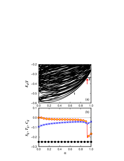
Figure 14: (Color online) (a) Energy spectrum per bond for a tetrahedral cluster as a function of $\alpha$ for $\eta=0$. Ground–state degeneracies are as indicated, with $d=6$ at $\alpha=0$ and $d=150$ at $\alpha=1$. The arrow marks a transition in the nature of the (low–spin) ground state. (b) Spin ($S_{ij}$, filled circles), orbital ($T_{ij}$, empty circles), and spin–orbital ($C_{ij}$, $\times$) correlation functions on the $c$ bond of the tetrahedral cluster as functions of $\alpha$ for $\eta=0$.

We begin the systematic presentation of results by discussing the energy spectra at $\eta=0$ [Fig. 14(a)]. As soon as the degeneracies of the superexchange limit ($\alpha=0$) are broken, the spectrum becomes very dense, and remains so across almost the complete phase diagram until a level–crossing at $\alpha_{c}=0.92$. The ground–state energy for all intermediate values of $\alpha$ interpolates smoothly towards the transition, showing an initial decrease not observed in the triangle: for the tetrahedron, mixed hopping terms make a significant contribution, leading to an overall energy minimum around $\alpha=0.15$. The dominance of these terms is indicated by both the extremely high value of $\alpha_{c}$ and the steepness of the low–$\alpha$ curve where the transition to the static VB phase is finally reached.

The bond correlation functions shown in Fig. 14(b) illustrate the effects of corrections to the VB ansatz. The spin correlations always have the constant value $S_{ij}=-\frac{1}{4}$, which is the most important indication of the breaking of symmetry between (ss/ot) and (os/st) sectors at low $\alpha$: this value is an average over the spin–singlet result $-3/4$ (on two bonds) and four bonds with value 0, and thus it is clear that (ss/ot) dimers afford more resonance energy. However, the proximity of (os/st) states suggests that a low value of $\eta_{c}$, the critical Hund coupling for the transition to the high–spin state, is to be expected (below).

The orbital correlations average to zero at $\alpha=0$, a non–trivial result whose origin lies in the breaking of nine–fold degeneracy within the orbital sector, and remain close to this value until the transition at $\alpha_{c}$. It is worth noting here that $T_{ij}=0$ implies a higher frustration in the orbital sector than would be obtained in the spin sector for an (os/st) state ($S_{ij}=-\frac{1}{12}$), which is due to the complex direction–dependence of the orbital degrees of freedom. This phase is maintained across much of the phase diagram, with only small changes to the correlation functions, the negative value of $T_{ij}$ reflecting an easing of orbital frustration. The lack of a phase transition throughout the region in which mixed processes are also important suggests that a dimer–based schematic picture of the ground state remains appropriate for the four–site system, with only quantitative evolution as a function of $\alpha$ until $\alpha_{c}=0.92$. At $\alpha=1$, the result $T_{ij}=-\frac{1}{6}$ is the consequence of $c$–orbital operators on the interdimer $a$ and $b$ bonds.

Significant spin–orbital correlations, $C_{ij}\simeq-0.1$ at $\alpha=0$ [Fig. 14(b)], are found to be due exclusively to the four–operator term at low $\alpha$. While these negative contributions drop steadily through most of the regime $\alpha<\alpha_{c}$, signifying a gradual decoupling of orbitals and spins as the static limit ($\alpha=1$) is approached, near $\alpha_{c}$ the negative value of $C_{ij}$ is again enhanced by the contribution $-S_{ij}T_{ij}$ due to the interdimer bonds. Thus, as for the triangle (Sec. V.3), the entanglement is finite, complete factorization is not possible, and a finite value $C_{ij}=-\frac{1}{24}$ is found even at $\alpha=1$. We note here that on the tetrahedron there is little information in the orbital occupations, which are constant ($n_{\gamma}=\frac{1}{3}$) over the entire phase diagram, demonstrating only the symmetry of this cluster geometry, and are therefore not shown.

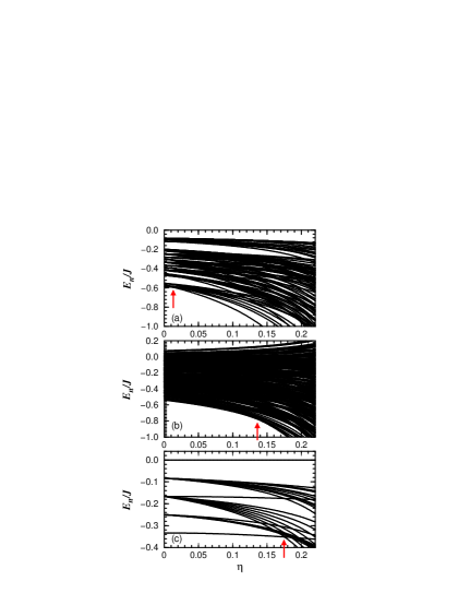
Figure 15: (Color online) Energy spectra for a tetrahedral cluster as a function of Hund exchange $\eta$. Energies are quoted per bond, and shown for: (a) $\alpha=0$, (b) $\alpha=0.5$, and (c) $\alpha=1$. The arrows indicate transitions from the low–spin ($S=0$) to the high–spin ($S=2$) ground state.

The spectra as a function of Hund coupling $\eta$ are shown for the three parameter choices $\alpha=0$, 0.5, and 1 in Fig. 15. Once again, the spectra become very dense away from $\eta=0$. At $\alpha=0$ [Fig. 15(a)] high–spin states are found also in the low–energy sector, as a consequence of the near–degeneracy of (ss/ot) and (os/st) states, and the high–spin transition occurs at a very low value of $\eta_{c}$ [Fig. 15(a)]. The direct–exchange limit is both qualitatively and quantitatively different, because the quantum fluctuations and the corresponding energy gains are limited to the spin sector, making the low–spin states considerably more stable and giving $\eta_{c}=0.175$ [Fig. 15(c)]. The spin excitation gap decreases gradually with increasing $\eta$, but until just below $\eta_{c}$, for all values of $\alpha$, the spin excitation is to $S=1$ states. However, these triplet states are never the ground state in the entire regime of $\eta$, a single transition always occurring directly into an $S=2$ state. In the intermediate regime represented by $\alpha=0.5$, the energy spectrum is so dense that individual states are difficult to follow (a more systematic analysis of the spectra in different subspaces of $S^{z}$ is not presented here). The high–spin transition occurs at the relatively high value $\eta_{c}=0.136$, due mainly to the large energy gains in the low–spin sector from mixed exchange. Further evidence for the importance of the orbital excitations in ${\cal H}_{m}$ (24) can be found in the broadening of the spectrum which leads to the occurrence of quantum states with weakly positive energies: for both superexchange and direct–exchange processes, the Hamiltonians are constructed as products of projection operators with negative coefficients, so positive energies are excluded.

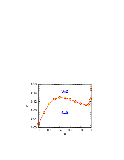
Figure 16: (Color online) Phase diagram of the tetrahedral cluster in the plane $(\alpha,\eta)$. As for the triangular cluster, the spin states below and above the line $\eta_{c}(\alpha)$ are respectively singlet ($S=0$) and quintet ($S=2$), with no intermediate triplet phase.

The low– to high–spin transition points at all values of $\alpha$ can be collected to give the full phase diagram of the tetrahedron shown in Fig. 16. As shown above, in the superexchange limit the high–spin state lies very close to the low–spin ground state, and the transition to an $S=2$ spin quintet occurs at $\eta_{c}=0.017$. We comment here that this high–spin state is in no sense classical or trivial, being based on orbital singlets which are stabilized by strong orbital fluctuations, and emphasize again that the high–spin sector also contains a manifold of rich problems in orbital physics, which we will not consider further here. The near degeneracy of (ss/ot) and (os/st) states is further lifted in the presence of the mixed terms in ${\cal H}_{m}$, raising $\eta_{c}$ to values on the order of 0.12 across the bulk of the phase diagram. For no choice of parameters is a spin triplet state found at intermediate values of $\eta$. The reentrant behavior close to $\alpha=0.5$ is an indication of the importance of mixed terms in stabilizing a low–spin state, the tetrahedral geometry providing one of the few examples we have found of anything other than a direct competition, and hence an interpolation, between the two limiting cases. The rapid upturn in the limit of $\alpha\to 1$ reflects the anomalous stability of the static VB states in the direct–exchange limit. The very strong asymmetry of the transition line in Fig. 16 contrasts sharply with the near–symmetry about $\alpha=0.5$ observed for the triangle (Fig. 13), and shows directly the differences between those features of the phase diagram which are universal and those which are effects of even or odd cluster sizes in a dimer–based system.

We close our discussion of the tetrahedral cluster with a brief discussion of degeneracies and summary of the picture provided by the VB ansatz with additional resonance. For the orbital occupation correlations and degeneracies, we begin with the low–spin sector ($\eta=0$). At $\alpha=0$ one has two (ss/ot) VBs resonating around the 6 bonds of the cluster, a state characterized by $P=1/6$, $Q=1/3$, and $R=1/2$; however, a mixing of the orbital triplet states lowers the degeneracy from 9 to $d=6$. For $\alpha>0$ the state is the same, with slow evolution of $P<1/6$, $Q>1/2$, and $R>1/3$, but now mixed hopping terms break all orbital degeneracies, giving $d=1$. Only when $\alpha>0.92$ is the ground state more accurately characterized as one based on spin singlets of the bond color, with significant values of $P$ and the restoration of an orbital degeneracy $d=2$. As $\alpha\rightarrow 1$, the diagonal hopping component is strengthened ($P\rightarrow 1/3$) as the pair of bond–colored spin singlets resonates, until at $\alpha=1$ they become static and the degeneracy is $d=3$.

For the high–spin states in the regime $\eta>\eta_{c}$, at $\alpha=0$ one has two resonating (os/st) VBs, with the hopping channels unchanged and only the spin degeneracy $d=5$. This state is not altered qualitatively for any $\alpha<0.92$, a transition value independent of $\eta$. For $0.92<\alpha<1$, orbital correlations are strongly suppressed and the state is characterized by hopping processes largely of the avoided–blocking type (one active orbital, $Q$ dominant), still with $d=5$. Finally, $\alpha=1$ represents the limit of a pure avoided–blocking state ($P=0$, $Q=2/3$, $R=1/3$), where the degeneracy jumps to 150, a number which can be understood as 5 (spin degeneracy) $\times$ [6 (number of two–color states with no bonds requiring spin singlets) + 24 (number of three–color states with no bonds requiring spin singlets)].

V.5 Four–site chain

As a fourth and final case, we present results from a linear four–site cluster. While not directly relevant to the study of the triangular lattice, this system offers further valuable insight into the intrinsic physics of the spin–orbital model. The cluster is oriented along the $c$–axis with periodic boundary conditions. As for the single bond (Sec. VB), only the $a$ and $b$ orbitals contribute at $\alpha=0$, where indeed one finds average electron densities per site $n_{ia}=n_{ib}=\frac{1}{2}$, and $n_{ic}=0$. Likewise, at $\alpha=1$ only the $c$ orbitals are occupied, with $n_{ic}=1$, a result dictated by the spin singlet correlations, which are fully developed only for complete orbital occupation.

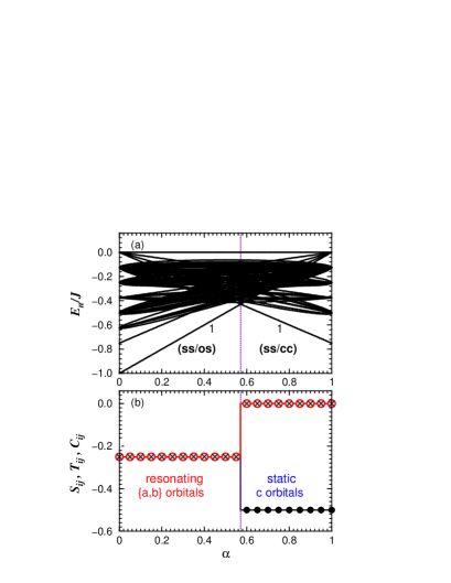
Figure 17: (Color online) Evolution of the properties of the four–site chain as a function of $\alpha$ at $\eta=0$: (a) energy spectrum and (b) spin ($S_{ij}$, filled circles), orbital ($T_{ij}$, empty circles), and spin–orbital ($C_{ij}$, $\times$) correlation functions. Both panels show a transition occurring at a level crossing at $\alpha=4/7$. In panel (a), the labels show a nondegenerate ground state ($d=1$) in both regimes, which has prediminantly spin singlet character at $\alpha>0.571$, but both spin and orbital singlet components at $\alpha<0.571$. In panel (b), $S_{ij}=T_{ij}=C_{ij}=-\frac{1}{4}$ for $\alpha<0.571$ due to a resonating $(ab)$ orbital configuration, while $T_{ij}=C_{ij}=0$ for $\alpha>0.571$ as a consequence of the static $c$ orbital configuration.

The energy per bond for the four–site chain in the superexchange limit is again $-J$, as for a single bond [Fig. 17(a)]: somewhat surprisingly, the bonds do not ”disturb” each other, and joint spin–orbital fluctuations extend over the entire chain. However, in contrast to a single bond, this behavior is due to only one quantum state, the SU(4) singlet. In this geometry, only one SU(2) orbital subsector is selected, and the resulting SU(2)$\otimes$SU(2) system is located precisely at the SU(4) point of the Hamiltonian.riqa Thus, exactly as in the SU(4) chain, all spin, orbital and spin–orbital correlation functions are equal, $S_{ij}=T_{ij}=C_{ij}=-0.25$, as shown in Fig. 17(b). For $S_{ij}$ and $T_{ij}$, this result may be understood as an average over equal probabilities of singlet and triplet states on each bond. In more detail, the condition set on the correlation functions by SU(4) symmetryFri99 is $\frac{4}{3}\langle({\vec{S}}_{i}\!\cdot\!{\vec{S}}_{j})({\vec{T}}_{ic}\!\cdot\!{\vec{T}}_{jc})\rangle=S_{ij}=T_{ij}$, an equality also obeyed by the single bond (Sec. VB). The product of $S_{ij}$ and $T_{ij}$ in its definition ensures the identity for $C_{ij}$. The unique ground state is nevertheless a linear superposition of states expressed in the spin and orbital bases, and has not only finite but maximal entanglement. This state persists, with a perfectly linear $\alpha$–dependence, all the way to $\alpha=1$, but ceases to be the ground state at $\alpha=\frac{4}{7}$ [Fig. 17(a)], where there is a level–crossing with the $\alpha=1$ ground state (also perfectly linear). This latter state has a completely different, fluctuation–free orbital configuration, with pure $c$–orbital occupation at every site, and gains energy solely in the direct–exchange channel. The spins and orbitals are decoupled, $T_{ij}$ and $C_{ij}$ vanish, and the spin state has $S_{ij}=-0.50$: this result can be understood as an equal average over bond states with ${\vec{S}}_{i}\cdot{\vec{S}}_{j}=-\frac{3}{4}$ and $-\frac{1}{4}$, and matches that obtained for the four–site AF Heisenberg model with a resonating VB (RVB) ground state.Faz99 The energy at $\alpha=1$, $E_{0}=-0.75J$ [Fig. 17(a)], is given directly by including the constant term, $-\frac{1}{4}J$ per bond, in the definition of the Hamiltonian (23).

The results for the linear four–site cluster demonstrate again the competition between superexchange and direct exchange. The orbital fluctuations arising due to the mixed exchange term, ${\cal H}_{m}$ (24), are responsible for removing the high degeneracies of the eigenenergies in the limits $\alpha=0$ and $\alpha=1$ [Fig. 17(a)]. In fact the spectrum of the excited states is quasi–continuous in the regime around $\alpha=0.5$, but has a finite spin and orbital gap everywhere other than the quantum critical point at $\alpha=\frac{4}{7}$.

These chain results raise a further possibility for the spontaneous formation at $\alpha=0$ of a 1D state not discussed in Sec. III. A set of (for example) $c$–axis chains, with only $a$ and $b$ orbitals occupied in the pseudospin sector, would create exactly the 1D SU(4) model, and would therefore redeem an energy $E=-\frac{3}{4}J$ per bond from the formation of linear, four–site spin–orbital singlets. The energy of the triangular lattice would receive a further, constant contribution from the cross–chain bonds, which was calculated in Eq. (35) for general $\eta$, and hence would be given at $\eta=0$ by

$$E_{\rm 1D}^{SU(4)}(0)=-\frac{1}{3}\cdot\frac{3}{4}J-\frac{1}{6}J\;=\;-\frac{5}{12}J.$$ (98)

This energy represents a new minimum compared with all of the results in Sec. III. That it was obtained from a melting of both spin and orbital order confirms the conclusion that ordered phases are inherently unstable in this class of model, being unable to provide sufficient energy to compete with the kinetic energy gains available through resonance processes. That its value is now lower than that obtained for a static, 2D dimer covering (Sec. IV) is not of any quantitative significance, given the results of Sec. V confirming the importance of the positional resonance of dimers.

V.6 Summary

To summarize, we have shown in this section the results of exact numerical diagonalization calculations performed on small clusters. Detailed analysis of ground–state energies, degeneracies, site occupancies and a number of correlation functions can be used to extract valuable information about the local physics of the model across the full regime of parameters. Essentially all of the quantities considered show strong local correlations and the dominance of quantum fluctuations of the shortest range, with ready explanations in terms of resonating dimer states.

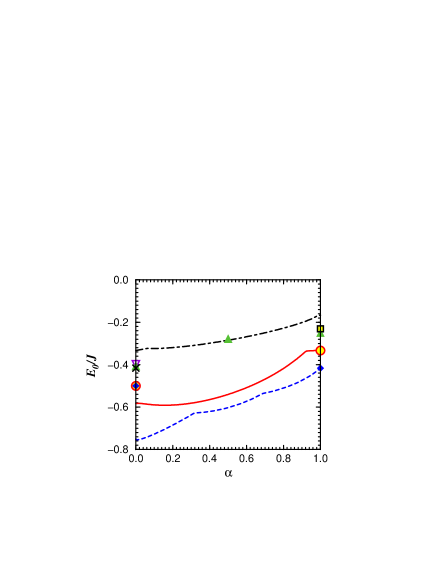
Figure 18: (Color online) Ground–state energy per bond as a function of $\alpha$, obtained with $\eta=0$ for a triangular cluster with 3 bonds (blue, dashed line), and a tetrahedral cluster with 6 bonds (red, solid line). For comparison, the energies obtained from the VB ansatz in the limiting cases $\alpha=0$ and $\alpha=1$ are shown for the triangular cluster (blue, diamonds) and tetrahedral cluster (red, yellow–filled, open circles); at $\alpha=0$ both VB energies are the same, while at $\alpha=1$ they match the exact solutions. Green, upward–pointing triangles show the static–dimer results of Sec. IV for the extended system, and the black, dot–dashed line the lowest energy per bond obtained for fully spin and orbitally ordered phases in Sec. III. The violet, downward–pointing triangle shows the energy of the orbitally ordered but spin–disordered Heisenberg–chain state at $\alpha=0$ [Eq. (35)] and the open, yellow–filled square that of the analogous state at $\alpha=1$ [Eq. (48)], while the cross shows the energy of the spin– and orbitally disordered, SU(4)–chain state [Eq. (98)].

We draw particular attention to the extremely low ground–state energy of the triangular cluster, which shows large gains from dimer resonance. The tetrahedral cluster also has a very significant resonance contribution, although more of its ground–state energy is captured at the level of a static dimer model. Such a VB ansatz provides the essential framework for the understanding of all the results obtained, even for systems with odd site numbers. The energies and their evolution with $\alpha$ contain some quantitative contrasts between even– and odd–site systems, allowing further insight concerning the range over which the qualitative features of the cluster results extend.

Focusing in detail upon these energies, Fig. 18 summarizes the exact diagonalization results at zero Hund coupling, and provides a comparison not only with the VB ansatz, but with all of the other results obtained in Secs. III–V. From bottom to top are shown: the exact cluster energies including all physical processes; the cluster VB ansatz, showing the importance of dimer resonance energy; the static VB ansatz for extended systems, suggesting by comparison with clusters the effects of resonance; the energies of “melted” states with 1D spin (and orbital) correlations; the optimal energy of states with full, long–ranged spin and orbital order.

Returning to the cluster results, their degeneracies can be understood precisely, and demonstrate the restoration of various symmetries due to resonance processes. We provide a complete explanation for all the correlation functions computed, and use these to quantify the entanglement as a function of $\alpha$, $\eta$ and the system size. There is a high–spin transition as a function of $\eta$ for all values of $\alpha$, which sets the basic phase diagram and establishes a new set of disentangled orbital models at high $\eta$.

The extrapolation of the cluster results to states of extended systems, some approximations for which are shown in Fig. 18, is not straightforward, and cannot be expected to include any information relevant to subtle selection effects within highly degenerate manifolds of states. However, with the exception of the static–dimer regime around $\alpha=1$, our calculations suggest that nothing subtle is happening in this model over the bulk of the phase diagram, where the physics is driven by large energetic contributions from strong, local resonance processes.

VI Rhombic, honeycomb, and kagome lattices

In Sec. I we alluded to the question of different sources of frustration in complex systems such as the spin–orbital model of Eq. (9). More specifically, this refers to the relative effects of pure geometrical frustration, as understood for AF spin interactions, and of interaction frustration of the type which can arise in spin–orbital models even on bipartite lattices.Fei97 Because the interaction frustration depends in a complex manner on system geometry, no simple separation of these contributions exists. In this section we alter the lattice geometry to obtain some qualitative results with a bearing on this separation, by considering the same spin–orbital model on the three simple lattice geometries which can be obtained from the triangular lattice by the removal of active bonds or sites.

The geometries we discuss are rhombic, obtained by removing all bonds in one of the three triangular lattice directions [Fig. 19(a)], honeycomb, or hexagonal, obtained by removing every third lattice site [Fig. 19(b)], and kagome, obtained by removing every fourth lattice site in a 2$\times$2 pattern [Fig. 19(c)]. Simple geometrical frustration is removed in the rhombic and honeycomb cases, but for Heisenberg spin interactions the kagome geometry is generally recognized (from the ground–state degeneracy of both classical and quantum problems) to be even more frustrated than the triangular lattice. We consider only the $\alpha=0$ and $\alpha=1$ limits of the model, and $\eta=0$. We discuss the results for long–range–ordered states (Sec. III) and for static dimer states (Sec. IV) for all three lattice geometries. Here we do not enter into numerical calculations on small clusters, and comment only on those systems for which exact diagonalization may be expected to yield valuable information not accessible by analytical considerations.

  

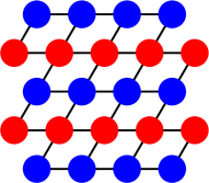
(a)                                    (b)

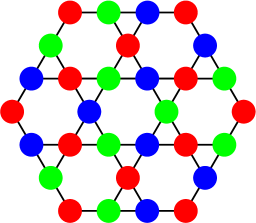
(c)

Figure 19: (Color online) (a) Rhombic lattice, showing a two–color orbitally ordered state. (b) Honeycomb lattice, showing a one–color orbitally ordered state. (c) Kagome lattice, showing a three–color orbitally ordered state.

VI.1 Rhombic lattice

While the connectivity of this geometry is precisely that of the square lattice, we refer to it here as rhombic to emphasize the importance of the bond angles of the chemical structure in maintaining the degeneracy of the $t_{2g}$ orbitals and in determining the nature of the exchange interactions. It is worth noting that the spin–orbital model (9) on this lattice may be realized in Sr₂VO₄ (below). In the absence of geometrical frustration, the spin problem created by imposing any fixed orbital configuration selected from Sec. III (Figs. 3 and 4) is generally rather easy to solve. Further, at $\eta=0$ both FM and AF, and by extension AFF, spin states have equal energies, leading to a high spin degeneracy.

Following Sec. III, the $\alpha=0$ energies for the majority of the orbitally ordered states of Fig. 3 are

$$E_{\rm lro}^{\rm rh}(0)=-\frac{1}{2}J$$ (99)

per bond at $\eta=0$ for a number of possible spin configurations, whose degeneracy is lifted (in favor of FM lines or planes) at finite $\eta$. Indeed, the only exceptions to this rule occur for the three–color state [Fig. 3(d)] and for orientations of the other states which preclude hopping in one of the two lattice directions, whose triangular symmetry properties are broken by the missing bond. As noted in Sec. III, for superpositions is it the exception rather than the rule for all hopping processes to be maximized, but on the rhombic lattice this is possible for the states in Fig. 4(a) and some orientations of those in Figs. 4(d) and 4(e).

For $\alpha=1$, the energy limit even on the triangular lattice was set rather by the number of active bonds than by the problem of minimizing their frustration. Similar to the $\alpha=0$ case, all states where the active hopping direction is one of the two lattice directions, plus in this case state (3d), can redeem the maximum energy available,

$$E_{\rm lro}^{\rm rh}(1)=-\frac{1}{4}J$$ (100)

at $\eta=0$, which is simply the avoided–blocking energy, for a large number of possible spin configurations. Finite Hund exchange favors FM spin states.

  

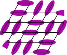
(a)                                (b)

Figure 20: (Color online) Rhombic lattice with (a) columnar and (b) plaquette dimer coverings.

Turning to dimerized states, the calculation of the energy of any given dimer covering proceeds as in Sec. IV, namely by counting for each the respective numbers of bonds of types (7a), (7b), and (7c) [Fig. 7]. For the rhombic lattice, lack of geometrical frustration means that all interdimer bonds can be chosen to be AF/AO. The two most regular dimer coverings of the rhombic lattice with small unit cells may be designated as “columnar” [Fig. 20(a)] and “plaquette” [Fig. 20(b)]. In both cases, $1/4$ of the bonds are the dimers, and by inspection $1/4$ of the interdimer bonds in the columnar state are of type (7a), while the remainder are (7c); by contrast, the plaquette state has no type–(7a) bonds, $1/2$ type–(7b) bonds, and the remainder are of type (7c). For $\alpha=0$, the energies are

$$E_{\rm dc}^{\rm rh}(0)\! = -\frac{1}{4}J-\frac{1}{4}\cdot\frac{1}{2}J-\frac{1}{2}\cdot\frac{1}{4}J\;=\;-\frac{1}{2}J,$$

$$E_{\rm dp}^{\rm rh}(0)\! = -\frac{1}{4}J-\frac{1}{2}\cdot\frac{3}{8}J-\frac{1}{4}\cdot\frac{1}{4}J\;=\;-\frac{1}{2}J$$ (101)

at $\eta=0$, both for (ss/ot) and for (os/st) dimers. The degeneracy of these two limiting cases, in the sense of maximal and minimal numbers of types–(7a) and –(7b) bonds, suggests a degeneracy of all dimer coverings at this level of analytical sophistication. Further, all of these dimer coverings are degenerate with all of the unfrustrated ordered states at $\eta=0$. The selection of a true ground state from this large manifold of static states (order–by–disorder) would hinge on higher–order processes, but these considerations are likely to be rendered irrelevant by dimer resonance (Sec. V).

For the spin–singlet dimer states at $\alpha=1$ one finds

$$E_{\rm dc}^{\rm rh}(1)\! = -\frac{1}{4}J-\frac{1}{4}\cdot\frac{1}{4}J-\frac{1}{2}\cdot 0J\;=\;-\frac{5}{16}J,$$

$$E_{\rm dp}^{\rm rh}(1)\! = -\frac{1}{4}J-\frac{1}{2}\cdot\frac{1}{4}J-\frac{1}{4}\cdot 0J\;=\;-\frac{3}{8}J,$$ (102)

at $\eta=0$, and thus that, as for the triangular lattice, the energy is minimized by dimer configurations excluding linear interdimer bonds. This remains a large manifold of dimer coverings, whose energy is manifestly lower than any of the possible orbitally ordered states in this limit of the model, and within which order–by–disorder is expected to operate (Sec. V).Jac07

The considerations of this subsection, extended to finite values of $\eta$, may be relevant in the understanding of experimental results for Sr₂VO₄. These suggest weak FM order,Noz91 accompanied by an AO orderTok05 which could be interpreted as arising from the formation of dimer pairs. When the oxygen octahedra distort, the threefold degeneracy of the $t_{2g}$ orbitals is lifted, to give a model containing only two degenerate orbitals, $d_{yz}$ and $d_{xz}$. This leads to a situation with Ising–like superexchange interactions and quasi–1D hole propagation in an effective $t$–$J$ model.Dag08

VI.2 Honeycomb lattice

The situation for the honeycomb lattice is very similar to that for the rhombic case. Again the absence of geometrical frustration makes it possible to obtain the minimal energy for a number of orbital orderings, with a high spin degeneracy at $\eta=0$. For pure superexchange interactions, once again

$$E_{\rm lro}^{\rm h}(0)=-\frac{1}{2}J$$ (103)

per bond, while in the direct–exchange limit

$$E_{\rm lro}^{\rm h}(1)=-\frac{1}{4}J,$$ (104)

both at $\eta=0$, for the same physical reasons as above.

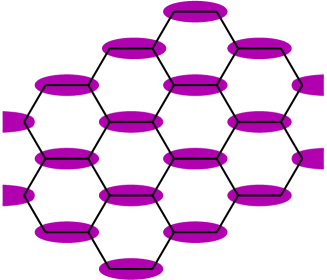
(a)

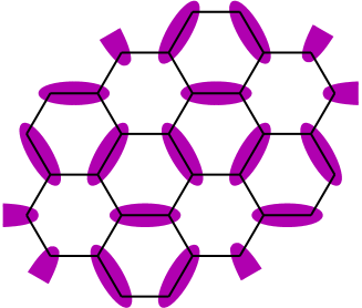
(b)

Figure 21: (Color online) Honeycomb lattice with (a) columnar and (b) three–way dimer coverings.

For dimer states, on the honeycomb lattice all interdimer bonds are by definition of type (7c), and again can be made AF/AO because frustration is absent, so the energies of all dimer coverings are de facto identical. By way of demonstration, the two simplest regular configurations, which we label “columnar” and “three–way”, are shown in Fig. 21, and, from the fact that now $1/3$ of the bonds contain dimers, their energies are

$$E_{\rm dc}^{\rm h}(0) = -\frac{1}{3}J-\frac{2}{3}\cdot\frac{1}{4}J\;=\;-\frac{1}{2}J,$$

$$E_{\rm d3}^{\rm h}(0) = -\frac{1}{3}J-\frac{2}{3}\cdot\frac{1}{4}J\;=\;-\frac{1}{2}J,$$ (105)

per bond at $\alpha=0=\eta$. Thus static dimer states are again degenerate with unfrustrated ordered states in the superexchange limit, and detailed consideration of kinetic processes would be required to deduce the lowest total energy. In this context, the dimer coverings shown in Fig. 21 exemplify two limits about which little kinetic energy can be gained from resonance (Fig. 21(a), where large numbers of dimers must be involved in any given process) and in which kinetic energy gains from processes involving short loops [the three dimers around 2/3 of the hexagons, Fig. 21(b)] are maximized.

At $\alpha=1$, only the dimer energy is redeemed, and this on $1/3$ of the bonds, so

$$E_{\rm d}^{\rm h}(1)=-\frac{1}{3}J$$ (106)

at $\eta=0$ for a large manifold of coverings. This energy is once again significantly better than any of the possible ordered states, a result which can be ascribed to the low connectivity. That the ground state of the extended system in this limit for both the rhombic and honeycomb lattices involves a selection from a large number of nearly degenerate states suggests that numerical calculations on small clusters would not be helpful in resolving detailed questions about its nature. The same model for the honeycomb geometry in the $\alpha=1$ limit has been discussed for the $S=1$ compound Li₂RuO₃,Jac08 where the authors invoked the lattice coupling, in the form of a structural dimerization driven by the formation of spin singlets, to select the true ground state.

VI.3 Kagome lattice

The kagome lattice occupies something of a special place among frustrated spin systemsDiep as one of the most highly degenerate and intractable problems in existence, for both classical and quantum spins, and even with only nearest–neighbor Heisenberg interactions. Interest in this geometry has been maintained by the discovery of a number of kagome spin systems, and has risen sharply with the recent synthesis of a true $S=1/2$ kagome material, ZnCu₃(OH)₆Cl₂.rsnbn Preliminary local–probe experimentsrinbsn ; rmea show a state of no magnetic order and no apparent spin gap, whose low–energy spin excitations have been interpretedrhea as evidence for an exotic spin–liquid phase. Both experimentally and theoretically, kagome systems of higher spins ($S=3/2$ and 5/2) are found to have flat bands of magnetic excitations, reflecting the very high degeneracy of the spin sector.rmgnyhlnl While no kagome materials are yet known with both spin and orbital degrees of freedom, Maekawa and coworkersKos03 ; Kha04 have considered the itinerant electron system on the triangular lattice for $\alpha=0$ (actually for the motion of holes in Na_xCoO₂), demonstrating that the combination of orbital, hopping selection, and geometry leads to any one hole being excluded from every fourth site, and thus moving on a system of four interpenetrating kagome lattices.

  

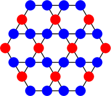
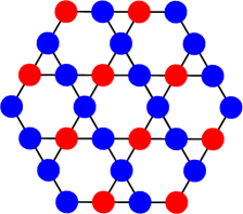
(a)                                (b)

Figure 22: (Color online) Kagome lattice with unequally weighted two–color states oriented (a) with and (b) against the lattice direction corresponding to the majority orbital color.

Considering first the energies per bond for states of long–ranged spin and orbital order, in a number of cases the values for the kagome lattice are identical to those of the triangular lattice. This is easy to show by inspection for the one–color state (3a), and for the superposition states (4a), (4b), and (4c), where bonds of all types are removed in equal number. However, for the less symmetrical orbital color configurations a more detailed analysis of the type performed in Sec. III is required, and yields provocative results. The two simple possibilities for ordered two–color states with a single color per site are shown in Fig. 22, and differ only in the orientation of the continuous lines (the majority color) relative to the active orbitals. These can be considered as the kagome–lattice analogs of states (3b) and (3c), as well as of (3e) and (3f).

When the lines of $c$–orbitals are aligned with the $c$–axis [Fig. 22(a)], this direction is inactive at $\alpha=0$, and only the other two directions contribute, one with two active FO orbitals, mandating an AF spin state to give energy $-\frac{1}{2}J$ per bond, and the other with energy $-\frac{1}{4}J$ and no strong spin preference, whence

$$E_{\rm(k3b)}(0)=-\frac{1}{4}J$$ (107)

at $\eta=0$ for sets of unfrustrated AF chains. By contrast, when the lines of $c$–orbitals fall along the $b$–direction [Fig. 22(b)], the $\alpha=0$ problem contains one FO and one AO line each with two active orbitals, and one line with one active orbital. Only the first requires AF spin alignment, while the other two lines are not frustrating, with the result that an energy

$$E_{\rm(k3c)}(0)=-\frac{5}{12}J$$ (108)

can be obtained. This value is lower than that on the triangular lattice, showing that for the class of models under consideration, where not all hopping channels are active in all directions, a system of lower connectivity can lead to frustration relief even when its geometry remains purely that of connected triangles.

With this result in mind, we consider again the possibilities offered by different three–color states, specifically those shown in Fig. 23. With reference to the superexchange problem, the state in Fig. 19(c), which by analogy with (3d) we denote as (k3d), contains only a small number of remnant triangles and isolated bonds still with two active orbitals. However, the state (k3d1), shown in Fig. 23(a) is that which ensures that no such bonds remain, and every single bond of the lattice has one active superexchange channel. The state (k3d2) in Fig. 23(b) is that in which every single bond of the lattice has two active (FO) superexchange channels: this possibility can be realized for the kagome geometry, at the cost of creating a frustrated magnetic problem requiring a 120^∘ spin state to minimize the energy,

$$E_{\rm(k3d)}(0) = -\frac{5}{16}J,$$ (109)

$$E_{\rm(k3d1)}(0) = -\frac{1}{4}J,$$ (110)

$$E_{\rm(k3d2)}(0) = -\frac{3}{8}J.$$ (111)

Thus one finds that lower energies than the value $-\frac{1}{3}J$ per bond, which was the lower bound for fully (orbitally and spin–)ordered states on the triangular lattice, are again possible for three–color ordered states. However, the residual spin frustration means that the lowest ordered–state energy on the kagome lattice is given by the unfrustrated, two–color AFF state, $E_{\rm(k3c)}(0)=-\frac{5}{12}J$.

  

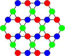
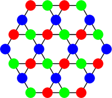
(a)                                (b)

Figure 23: (Color online) Kagome lattice with two different, equally weighted three–color states: (a) two–color lines oriented such that only one superexchange channel, plus the direct exchange channel, is active on every bond. (b) two–color lines oriented such that all superexchange channels are active, but no direct exchange channels.

We present briefly the energies of the same states at $\alpha=1$, where only a maximum of one hopping channel per bond can be active, and as noted above this is generally a stricter energetic limit than any frustration constraints. The results at $\eta=0$ are

$$E_{\rm(k3b)}(1)=-\frac{1}{4}J$$ (112)

for an AFF state gaining most of its energy from the $c$–axis chains, and

$$E_{\rm(k3c)}(1)=-\frac{1}{12}J$$ (113)

due to the dearth of active orbitals in this orientation. Similarly, by counting active orbitals in the three–color states,

$$E_{\rm(k3d)}(1) = -\frac{1}{6}J,$$ (114)

$$E_{\rm(k3d1)}(1) = -\frac{1}{4}J,$$ (115)

$$E_{\rm(k3d2)}(1) = 0,$$ (116)

and it is the state of Fig. 23(a) which achieves the unfrustrated value $-\frac{1}{4}J$ by permitting one active hopping channel on every bond of the kagome lattice.

We will not discuss the orbital superposition states which are the analogs of (4d) and (4e), noting only that these present again two different possibilities on the kagome lattice, depending on the orientation of the majority lines. Even with the frustration relief offered by this geometry for the type of model under consideration, superposition states contain too many hopping channels for all to be satisfied simultaneously, and it is not possible to equal the energy values found respectively for the configurations in Figs. 23(a) and (b) at $\alpha=1$ and $\alpha=0$.

It remains to consider dimer states on the kagome lattice, as these have been of equal or lower energy for every case analyzed so far. The set of nearest–neighbor dimer coverings of the kagome lattice is large, and for the $S=1/2$ Heisenberg model in this geometry the spin singlet manifold has been proposed as the basis for an RVB description.rmm Two dimer coverings degenerate at the level of the current treatment are shown in Fig. 24.

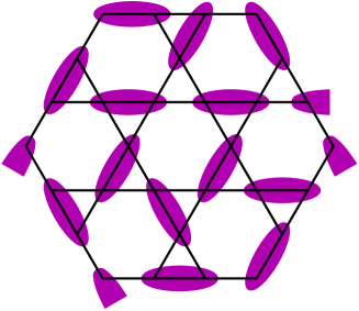
(a)

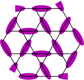
(b)

Figure 24: (Color online) Kagome lattice with two different dimer coverings, (a) and (b). In both examples, only two of the twelve triangles shown explicitly on the cluster are “defective” (contain no dimer), but the reader may notice that many of the next twelve triangles adjoining the boundary must also be so.

Dimer coverings of the kagome lattice have the property that $3/4$ of the triangles contain one dimer. In this case, the other bonds of the triangle are interdimer bonds, one of which is of type (7b) while the other is of type (7c). The other 1/4 of the triangles, knownre as “defect triangles”, have no dimers, and their three bonds are either all of type (7b), with probability 1/4, or one each of types (7a), (7b), and (7c), with probability 3/4. The frustration of the system is contained in the problem of minimizing the number of FM/FO interdimer bonds; this exercise is complex and no solution is known, so only an upper bound will be estimated here.

The bonds of a defect triangle connect three different dimers, and so one (or all three) must be FM/FO. A hexagon of the kagome lattice with no dimers on its bonds is surrounded by six non–defective triangles, one with one dimer by one defective neighbor, with two dimers two, and a hexagon with three dimers shares its non–dimer bonds with three defect triangles. Hexagons with odd dimer numbers must create a FM/FO bond between at least one pair of dimers, and it is reasonable to place this bond on the defect triangle(s) where an energy cost is already incurred. We note immediately that the cost of reversing the type–(7a) bond, $\frac{1}{4}J$ (Sec. IVA), exceeds that of reversing both interdimer bonds of a non–defective triangle, which is $\frac{1}{8}J+\frac{1}{16}J$. As a consequence, we take this cost, which is equal to that of reversing both a non–defective triangle and the weakest bond of the defect triangle, to be an upper bound on the effect of frustration. The net energy of a dimer state for $\alpha=0=\eta$ is then estimated to be

$$E_{\rm kd}(0)\!\! = -\frac{3}{4}\!\cdot\!\frac{1}{3}J-\frac{3}{4}\!\cdot\!\frac{1}{3}J\left(\frac{3}{8}+\frac{1}{4}\right)$$ (117)

$$-\frac{1}{4}J\left[\frac{1}{4}\!\left(\frac{2}{3}\!\cdot\!\frac{3}{8}\!+\!\frac{1}{3}\!\cdot\!\frac{1}{4}\right)\!+\!\frac{3}{4}\!\cdot\!\frac{1}{3}\!\left(\frac{1}{4}\!+\!\frac{3}{8}\!+\!\frac{1}{4}\right)\!\right]$$

$$= \!-\frac{209}{384}J\;\simeq\;-\frac{13}{24}J.$$

This is a very large number for the kagome lattice, exceeding even the value $-\frac{1}{2}J$ per bond (which, however, is of no special significance here). Thus we find that dimer states in this type of model are strongly favored, gaining a very much higher energy than even the best ordered states. Qualitatively, the dimer energy shares with the ordered–state energy the feature that it is considerably better than anything obtainable for the triangular lattice. This implies that the reduced connectivity of the lattice geometry for a model where the orbital degeneracy provides a number of mutually exclusive hopping channels makes it easier to find states where every remaining bond can support a favorable hopping process without strong frustration.

Applying all of the above geometrical considerations to the direct–exchange model ($\alpha=1$), where there is no frustration problem between the spin singlets, one finds

$$E_{\rm kd}(1) = -\frac{3}{4}\cdot\frac{1}{3}J-\frac{3}{4}\cdot\frac{1}{3}J\left[\frac{1}{4}+0\right]$$ (118)

$$-\frac{1}{4}\cdot\frac{1}{3}J\left[\frac{1}{4}\cdot\frac{3}{4}+\frac{1}{4}\cdot\frac{1}{2}\right]$$

$$= -\frac{21}{64}J$$

at $\eta=0$. Once again this energy is significantly lower than the value $E_{\rm dim}(1)=-\frac{1}{4}J$ obtained for the triangular lattice in Eq. (83), demonstrating that the multichannel spin–orbital model of the type considered here is less frustrated in the kagome geometry.

We comment in closing that the dimer energies we have estimated are only those of static VB configurations, and, away from $\alpha=1$, the possibility remains of a significant resonance energy gain from quantum fluctuations between these states (cf. Sec. V). Numerical calculations on small clusters of sufficient size (here at least 6 sites for a unit cell) would be helpful in this frustrated case.

To summarize this section, the spin–orbital model on bipartite lattices appears to present competing ordered and dimerized states with the prospect of high degeneracies. Among “frustrated” systems (in the sense of being non–bipartite), the kagome lattice provides an example where geometrical and orbital frustration effects cancel partially, affording favorable dimerized solutions. Thus, while it is possible to ascribe some of the frustration effects we have studied in the triangular lattice to a purely geometrical origin, for more complex models it is in general necessary to extend the concept of “geometrical frustration” beyond that applicable to pure spin systems.

VII Discussion and summary

We have considered a spin–orbital model representative of a strongly interacting $3d^{1}$ electron system with the cubic structural symmetry of edge–sharing metal–oxygen octahedra, conditions which lead to a triangular lattice of magnetic interactions between sites with unbroken, threefold orbital degeneracy. We have elucidated the qualitative phase diagram, which turns out to be very rich, in the physical parameter space presented by the ratio ($\alpha$) of superexchange to direct–exchange interactions and the Hund exchange ($\eta$).

Despite the strong changes in the fundamental nature of the model Hamiltonian as a function of $\alpha$ and $\eta$, a number of generic features persist throughout the phase diagram. With the exception of the ferromagnetic phases at high $\eta$, which effectively suppresses quantum spin fluctuations (below), there is no long–ranged magnetic or orbital order anywhere within the entire parameter regime. This shows a profound degree of frustration whose origin lies both in the geometry and in the properties of the spin–orbital coupling; a qualitative evaluation of these respective contributions is discussed below.

All of the phases of the model show a strong preference for the formation of dimers. This can be demonstrated in a simple, static valence–bond (VB) ansatz, and is reinforced by the results of numerical calculations. The static ansatz is already an exact description of the direct–exchange limit, $\alpha=1$, and gives the best analytic framework for understanding the properties of much of the remainder of the phase diagram. The most striking single numerical result is the prevalence of VB states even on a triangular cluster, and the underlying feature reinforced by all of the calculations is the very large additional “kinetic” contribution to the ground–state energy arising from the resonance of VBs due to quantum fluctuations. It is this resonance which drives symmetry restoration in some or all of the spin, orbital, and translational sectors over large regions of the parameter space. The sole exception to dimerization is found at high $\eta$ and around $\alpha=1$, where the only mechanism for virtual hopping is the adoption of orbital configurations which permit one orbital to be active (“avoided blocking”).

The “most exotic” region of the phase diagram is that at small $\alpha$ and $\eta$, and this we have assigned tentatively as an orbital liquid. In this regime, quantum fluctuations are at their strongest and most symmetrical, and every indication obtained from energetic considerations of extended systems, and from microscopic calculations of a range of local quantities on small clusters, suggests a highly resonant, symmetry–restored phase. While this orbital liquid is in all probability (again from the same indicators) based on resonating dimers, an issue we discuss in full below, we cannot exclude fully the possibility of a type of one–dimensional physics: short, fluctuating segments of frustration–decoupled spin or orbital chains, whose character persists despite the high site coordination. It should be stressed here that the point $(\alpha,\eta)$ = (0,0) is not in any sense a parent phase for exotic states in the rest of the phase diagram: mixed and direct exchange processes are qualitatively different elements, which introduce different classes of frustrated model at finite $\alpha$. While the matter is somewhat semantic, we comment only that one cannot argue for the point $\alpha=0.5$ being “more exotic” than $\alpha=0$ despite having the maximal number of equally weighted hopping channels, because it does not possess any additional symmetries which mandate qualitative changes to the general picture. In this sense, the limit $\alpha=1$ serves as a valuable fixed point which is understood completely, and yet is still dominated by the purely quantum mechanical concept of singlet formation.

One indicator which can be employed to quantify “how exotic” a phase may be is the entanglement of spin and orbital degrees of freedom. We define entanglement as the deviation of the spin and orbital sectors from the factorized limit in which their fluctuations can be treated separately. We compute a spin–orbital correlation function and use it to measure entanglement, finding that this is significant over the whole phase diagram. Qualitatively, entanglement is maximal around the superexchange limit, which is dominated by dimers where singlet formation forces the other sector to adopt a local triplet state. However, for particular clusters and dimer configurations, the high symmetry may allow less entangled possibilities to intervene exactly at $\alpha=0$. The direct–exchange limit, $\alpha=1$, provides additional insight into the entanglement definition: the four–operator spin–orbital correlation function vanishes, reflecting the clear decoupling of the two sets of degrees of freedom at this point, but the finite product of separate spin and orbital correlation functions violates the factorizability condition.

This preponderance of evidence for quantum states based on robust, strongly resonating dimers implies further that the (spin and orbital) liquid phase is gapped. Such a state would have only short–ranged correlation functions. However, these gapped states are part of a low–energy manifold, and for the extended system we have shown that this consists quite generally of large numbers of (nearly) degenerate states. The availability of arbitrary dimer rearrangements at no energy cost has been suggested to be sufficient for the deconfinement of elementary $S=1/2$ (and by analogy $T=1/2$) excitations with fractional statistics.rdmnm However, the spinons (orbitons) are massive in such a model, in contrast to the properties of algebraic liquid phases.rhsf

A low–spin to high–spin transition, occurring as a function of $\eta$, is present for all values of $\alpha$. The quantitative estimation of $\eta_{c}$ in the extended system remains a problem for a more sophisticated analysis. At the qualitative level, large $\eta$ can be considered to suppress quantum spin fluctuations by promoting parallel–spin (ferromagnetic) intermediate states on the magnetic ions. However, even when this sector is quenched, the orbital degrees of freedom remain frustrated, and contain non–trivial problems in orbital dynamics. In the superexchange (low–$\alpha$, high–$\eta$) region, frustration is resolved by the formation of orbital singlet (spin triplet) dimers, whose resonance minimizes the ground–state energy. The frustration in the direct–exchange (high–$\alpha$, high–$\eta$) region is resolved by avoided–blocking orbital configurations, and order–by–disorder effects are responsible for the selection of the true ground state from a degenerate manifold of possibilities; this is the only part of the phase diagram not displaying dimer physics. Thus the ferromagnetic orbital models in both limits exhibit a behavior quite different from that of systems with only $S=1/2$ spin degrees of freedom on the triangular lattice.

We have commented on both geometry and spin–orbital interactions as the origin of frustration in the models under consideration. However, a statement such as “on the triangular lattice, geometrical frustration enhances interaction frustration for spin–orbital models” must be qualified carefully. We have obtained anecdotal evidence concerning such an assertion in Sec. VI by considering other lattice geometries, and find that indeed the same model on an unfrustrated geometry appears capable of supporting ordered states; however, the interplay of the two effects is far from direct, as the kagome lattice presents a case where dimer formation acts to reduce the net frustation. Quite generally, spin–orbital models contain in principle more channels which can be used for relieving frustration, but the exact nature of the coupling of spin and orbital sectors may result in the opposite effect. Specific data characterizing mutual frustration can be obtained from the spin and orbital correlations computed on small clusters: as shown in Sec. V, for the triangular lattice there are indeed regimes where, for example, the effective orbital interactions enforced by the spin sector make the orbital sector more frustrated (higher $T_{ij}$) than would be the analogous pure spin problem (measured by $S_{ij}$), and conversely.

We comment briefly on other approaches which might be employed to obtain more insight into the states of the extended system, with a view to establishing more definitively the nature and properties of the candidate orbital liquid phase. More advanced numerical techniques could be used to analyze larger unit cells, but while Lanczos diagonalization, contractor renormalizationrclm or other truncation schemes might afford access to systems two, or even four, times larger, it seems unlikely that these clusters could provide the qualitatively different type of data required to resolve the questions left outstanding in Sec. V. An alternative, but still non–perturbative and predominantly unbiased, approach would be the use of variational wave functions, either formulated generally or in the more specific projected wave function technique which leads to different types of flux phase.rh ; rrhlw Adapting this type of treatment to the coupled spin and orbital sectors without undue approximation remains a technical challenge.

Within the realm of effective models which could be obtained by simplification of the ground–state manifold, we cite only the possibility motivated by the current results of constructing dimer models based on (ss/ot) and (os/st) dimers. Dimer modelsRok88 are in general highly simplified, and there is no systematic procedure for their derivation from a realistic Hamiltonian, but they are thought to capture the essential physics of certain classes of dimerized systems. Because QDM Hamiltonians provide exact solutions, and in some cases genuine examples of exotica long sought in spin systems, including the RVB phase and deconfined spinon excitations, they represent a valuable intermediate step in understanding how such phenomena may emerge in real systems. Here we have found (i) a very strong tendency to dimer formation, (ii) a large semi–classical degeneracy of basis states formed from these dimers, and (iii) that resonance processes even at the four–site plaquette scale provide a very significant energetic contribution. From the final observation alone, a minimal QDM, meaning only exchange of parallel dimers of all three directions and on all possible plaquette units, would already be expected to contain the most significant corrections to the VB energy. At this point we emphasize that, because of the change of SU(2) orbital sector with lattice direction, our 2D models are not close to the SU(4) point where four–site plaquette formation, and hence very probably a crystallization, would be expected.rpmfm From the results of Secs. IV and V, a rather more likely phase of the QDM would be one with complete plaquette resonance through all three colors, and without breaking of translational symmetry.

Rigorous proof of a liquid phase, such as that represented by an RVB state, is more complex, and as noted in Sec. I it requires satisfying both energetic and topological criteria. Following the prescription in Ref. Mil07, , three conditions must be obeyed: (i) a propensity for dimer formation, (ii) a highly degenerate manifold of basis states from which the RVB ground state may be constructed, and (iii) a mapping of the system to a liquid phase of a QDM. Criteria (i) and (ii) match closely the labels in the previous paragraph, and both dimer formation and high degeneracy have been demonstrated extensively here. The energetic part of criterion (iii) also appears to be obeyed here: static dimers have an energy ($V$), and allowing their location and orientation to change gains more ($t$). The regime $V/t<1$ of the triangular–lattice QDM is the RVB phase demonstrated in Ref. Moe01, , whose properties include short–range correlation functions and gapped, deconfined spinons. This mapping also contains the criterion of togological degeneracy, and could in principle be partially circumvented by a direct demonstration. However, no suitable numerical studies are available of non–simply connected systems, and so here we can present only plausibility arguments based on the high degeneracy and spatial topology of the dimer systems analyzed in Secs. IV and V. It is safe to conclude that the threefold–degenerate $t_{2g}$ orbital system on the triangular lattice is one of best candidates yet for a true spin–orbital RVB phase.

In closing, spin–orbital models have become a frontier of intense current interest for both experimental and theoretical studies of novel magnetic and electronic states emerging as a consequence of intrinsic frustration. Our model has close parallels to, and yet crucial differences from, similar studies of manganites (cubic systems of $e_{g}$ orbitals), LiNiO₂ (triangular, $e_{g}$), YTiO₃ and CaVO₃ (cubic, $t_{2g}$), and many other transition–metal oxides, appearing in some respects to be the most frustrated yet discussed. One of its key properties, arising from the extreme (geometrical and interaction–driven) frustration, is that ordered states become entirely uncompetitive compared to the resonance energy gained by maximizing quantum (spin and orbital) fluctuations. In the orbital sector, the restoration of symmetry by orbital fluctuations makes the model a strong candidate to display an orbital liquid phase. Because this liquid is based on robust dimer states, the mechanism for its formation is very likely to be spin–orbital RVB physics.

- (1) Frustrated Spin Systems, edited by H. T. Diep (World Scientific, Singapore, 2004).
- (2) P. Fazekas, Lectures on Electron Correlation and Magnetism (World Scientific, Singapore, 1999).
- (3) J. Zaanen, G. A. Sawatzky, and J. W. Allen, Phys. Rev. Lett. 55, 418 (1985).
- (4) A. M. Oleś, P. Horsch, G. Khaliullin, and L. F. Feiner, Phys. Rev. B72, 214431 (2005).
- (5) K. I. Kugel and D. I. Khomskii, Usp. Fiz. Nauk 136, 621 (1982) [Sov. Phys. Usp. 25, 231 (1982)].
- (6) C. Castellani, C. R. Natoli, and J. Ranninger, Phys. Rev. B18, 4945 (1985); Phys. Rev. B18, 4967 (1985); Phys. Rev. B18, 5001 (1985).
- (7) L. F. Feiner, A. M. Oleś, and J. Zaanen, Phys. Rev. Lett. 78, 2799 (1997).
- (8) J. B. Goodenough, Magnetism and the Chemical Bond (Interscience, New York, 1963); J. Kanamori, J. Phys. Chem. Solids 10, 87 (1959).
- (9) A. M. Oleś, P. Horsch, L. F. Feiner, and G. Khaliullin, Phys. Rev. Lett. 96, 147205 (2006).
- (10) Y. Q. Li, M. Ma, D. N. Shi, and F. C. Zhang, Phys. Rev. Lett. 81, 3527 (1998).
- (11) A. M. Oleś, P. Horsch, and G. Khaliullin, Phys. Stat. Solidi B 244, 3478 (2007).
- (12) B. Frischmuth, F. Mila, and M. Troyer, Phys. Rev. Lett. 82, 835 (1999); F. Mila, B. Frischmuth, A. Deppeler, and M. Troyer, ibid. 82, 3697 (1999).
- (13) K. Penc, M. Mambrini, P. Fazekas, and F. Mila, Phys. Rev. B68, 012408 (2003).
- (14) G. Khaliullin and S. Maekawa, Phys. Rev. Lett. 85, 3950 (2000); G. Khaliullin, Phys. Rev. B64, 212405 (2001).
- (15) J. van den Brink, New J. Phys. 6, 201 (2004).
- (16) G. Mihaly, I. Kezsmarki, F. Zamborszky, M. Miljak, K. Penc, P. Fazekas, H. Berger, and L. Forro, Phys. Rev. B61, R7831 (2000); P. Fazekas, K. Penc, K. Radnoczi, N. Barisic, H. Berger, L. Forro, S. Mitrovic, A. Gauzzi, L. Demko, I. Kezsmarki, and G. Mihaly, J. Magn. Magn. Mater. 310, 928 (2007).
- (17) P. Horsch, G. Khaliullin, and A. M. Oleś, Phys. Rev. Lett. 91, 257203 (2003).
- (18) F. Vernay, K. Penc, P. Fazekas, and F. Mila, Phys. Rev. B70, 014428 (2004); F. Vernay, A. Ralko, F. Becca, and F. Mila, ibid. 74, 054402 (2006).
- (19) F. Mila, F. Vernay, A. Ralko, F. Becca, P. Fazekas, and K. Penc, J. Phys.: Condens. Matter 19, 145201 (2007).
- (20) S. Di Matteo, G. Jackeli, C. Lacroix, and N. B. Perkins, Phys. Rev. Lett. 93, 077208 (2004); S. Di Matteo, G. Jackeli, and N. B. Perkins, Phys. Rev. B72, 024431 (2005).
- (21) S. Di Matteo, G. Jackeli, and N. B. Perkins, Phys. Rev. B72, 020408(R) (2005).
- (22) L. F. Feiner and A. M. Oleś, Phys. Rev. B71, 144422 (2005).
- (23) G. Khaliullin, Prog. Theor. Phys. Suppl. 160, 155 (2005).
- (24) P. Fazekas and P. W. Anderson, Philos. Mag. 30, 423 (1974).
- (25) F. Mila, Phys. Rev. Lett. 81, 2356, (1988); M. Mambrini and F. Mila, Eur. Phys. J. B 17, 651 (2000).
- (26) D. S. Rokhsar and S. A. Kivelson, Phys. Rev. Lett. 61, 2376 (1988).
- (27) R. Moessner and S. L. Sondhi, Phys. Rev. Lett. 86, 1881 (2001).
- (28) A. Ralko, M. Ferrero, F. Becca, D. Ivanov, and F. Mila Phys. Rev. B71, 224109 (2005).
- (29) A. Weisse and H. Fehske, New J. Phys. 6, 158 (2004); E. Dagotto, New J. Phys. 7, 67 (2005); K. Rościszewski and A. M. Oleś, J. Phys.: Cond. Matter 19, 186223 (2007).
- (30) P. Piekarz, K. Parlinski, and A. M. Oleś, Phys. Rev. Lett. 97, 156402 (2006); Phys. Rev. B76, 165124 (2007).
- (31) D. I. Khomskii and T. Mizokawa, Phys. Rev. Lett. 94, 156402 (2005).
- (32) M. Holzapfel, S. de Brion, C. Darie, P. Bordet, E. Chappel, G. Chouteau, P. Strobel, A. Sulpice, and M. D. Núñez–Regueiro, Phys. Rev. B70, 132410 (2004).
- (33) A. Reitsma, L. F. Feiner, and A. M. Oleś, New J. Phys. 7, 121 (2005).
- (34) M. V. Mostovoy and D. I. Khomskii, Phys. Rev. Lett. 89, 227203 (2002).
- (35) K. Hirakawa, H. Kadowaki, and K. Ubukoshi, J. Phys. Soc. Jpn. 54, 3526 (1985).
- (36) K. Takeda, K. Miyake, K. Takeda, and K. Hirakawa, J. Phys. Soc. Jpn. 61, 2156 (1992).
- (37) H. F. Pen, J. van den Brink, D. I. Khomskii, and G. A. Sawatzky, Phys. Rev. Lett. 78, 1323 (1997).
- (38) T. Motohashi, Y. Katsumata, T. Ono, R. Kanno, M. Karppinen, and H. Yamauchi, J. Appl. Phys. 103, 07C902 (2008).
- (39) M. Itoh, M. Shikano, H. Kawaji, and T. Nakamura, Solid State Commun. 80, 545 (1991); Y. Imai, I. Solovyev, and M. Imada, Phys. Rev. Lett. 95, 176405 (2005).
- (40) W. Koshibae and S. Maekawa, Phys. Rev. Lett. 91, 257003 (2003).
- (41) J. S. Griffith, The Theory of Transition Metal Ions (Cambridge University Press, Cambridge, 1971).
- (42) G. Khaliullin, P. Horsch, and A. M. Oleś, Phys. Rev. Lett. 86, 3879 (2001); A. M. Oleś, P. Horsch, and G. Khaliullin, Phys. Rev. B75, 184434 (2007).
- (43) A. B. Harris, T. Yildirim, A. Aharony, O. Entin-Wohlman, and I. Ya. Korenblit, Phys. Rev. Lett. 91, 087206 (2003).
- (44) This convenient notation for the triangular lattice was introduced by G. Khaliullin, W. Koshibae, and S. Maekawa, Phys. Rev. Lett. 93, 176401 (2004).
- (45) A. M. Oleś, Phys. Rev. B28, 327 (1983).
- (46) J. Zaanen and G. A. Sawatzky, J. Solid State Chem. 88, 8 (1990).
- (47) T. Mizokawa and A. Fujimori, Phys. Rev. B54, 5368 (1996).
- (48) M. Daghofer, A. M. Oleś, and W. von der Linden, Phys. Rev. B70, 184430 (2004); Phys. Stat. Solidi B 242, 311 (2005).
- (49) G. Jackeli and D. A. Ivanov, Phys. Rev. B76, 132407 (2007).
- (50) C. Itoi, S. Qin, and I. Affleck, Phys. Rev. B61, 6747 (2000).
- (51) A. Nozaki, H. Yoshikawa, T. Wada, H. Yamauchi, and S. Tanaka, Phys. Rev. B 43, 181 (1991).
- (52) J. Matsuno, Y. Okimoto, M. Kawasaki, and Y. Tokura, Phys. Rev. Lett. 95, 176404 (2005).
- (53) M. Daghofer, K. Wohlfeld, A. M. Oleś, E. Arrigoni, and P. Horsch, Phys. Rev. Lett. 100, 066403 (2008).
- (54) G. Jackeli and D. I. Khomskii, Phys. Rev. Lett. 100, 147203 (2008).
- (55) M. P. Shores, E. A. Nytko, B. M. Barlett, and D. G. Nocera, J. Am. Chem. Soc. 127, 13462 (2005).
- (56) T. Imai, E. A. Nytko, B. M. Bartlett, M. P. Shores, and D. G. Nocera, Phys. Rev. Lett. 100, 077203 (2008).
- (57) P. Mendels, F. Bert, M. A. de Vries, A. Olariu, A. Harrison, F. Duc, J. C. Trombe, J. S. Lord, A. Amato, and C. Baines, Phys. Rev. Lett. 98, 077204 (2007); F. Bert, S. Nakamae, F. Ladieu, D. L’Hôte, P. Bonville, F. Duc, J.–C. Trombe, and P. Mendels, Phys. Rev. B76, 132411 (2007); A. Olariu, P. Mendels, F. Bert, F. Duc, J.–C. Trombe, M. A. de Vries, and A. Harrison, Phys. Rev. Lett. 100, 087202 (2008).
- (58) J. S. Helton, K. Matan, M. P. Shores, E. A. Nytko, B. M. Barlett, Y. Yoshida, Y. Takano, A. Suslov, Y. Qiu, J.–H. Chung, D. G. Nocera, and Y. S. Lee, Phys. Rev. Lett. 98, 107204 (2007).
- (59) K. Matan, D. Grohol, D. G. Nocera, T. Yildirim, A. B. Harris, S. H. Lee, S. Nagler, and Y. S. Lee, Phys. Rev. Lett. 96, 247201 (2006).
- (60) V. Elser, Phys. Rev. Lett. 62, 2405 (1989).
- (61) S. Dommange, M. Mambrini, B. Normand, and F. Mila, Phys. Rev. B68, 224416 (2003).
- (62) M. Hermele, T. Senthil, and M. P. A. Fisher, Phys. Rev. B72, 104404 (2005).
- (63) S. Capponi, A. Läuchli, and M. Mambrini, Phys. Rev. B70, 104424 (2004).
- (64) M. B. Hastings, Phys. Rev. B63, 014413 (2000).
- (65) Y. Ran, M. Hermele, P. A. Lee, and X.–G. Wen, Phys. Rev. Lett. 99, 117205 (2007).