CANGAROO-III Search for Gamma Rays from Kepler’s Supernova Remnant

Abstract

Kepler’s supernova, discovered in October 1604, produced a remnant that has been well studied observationally in the radio, infrared, optical, and X-ray bands, and theoretically. Some models have predicted a TeV gamma-ray flux that is detectable with current Imaging Cherenkov Atmospheric Telescopes. We report on observations carried out in 2005 April with the CANGAROO-III telescope. No statistically significant excess was observed, and limitations on the allowed parameter range in the model are discussed.

1. Introduction

Kepler’s supernova remnant (SNR) (G4.5+6.8) is 400 years old (Blair, 2005, see for review) and provides an unrivaled opportunity to verify the belief that supernova remnants are the origin of Galactic cosmic rays. Cas A is younger (by $\sim$60 years) and was detected at TeV $\gamma$-ray energies (Aharonian et al., 2001), which implies the acceleration of high-energy cosmic rays. Older remnants, such as RX J0852.0-4622 (Katagiri et al., 2005; Aharonian et al., 2005; Enomoto et al., 2006b) and RX J1713.7-3946 (Enomoto et al., 2002a; Aharonian et al., 2004), both thought to be 1,000$\sim$2,000 years old, have also been detected. If SNR age was the dominant factor in for cosmic-ray acceleration, one might expect similar levels of cosmic ray acceleration in Kepler’s SNR. Of course, other variables, such as SN type, local environment, and distance, will certainly have some impact on the likelihood of TeV gamma-ray detection from a SNR.

Kepler’s SN was considered to be a type Ia supernova (SN) based on an interpretation of the historical light curve (Baade, 1943). It was later shown that the light curve was also in agreement with a type II-L SN (Doggett & Branchi, 1985). However, recent observations of thermal X-ray emission by ASCA (Kinugasa & Tsunemi, 2007) and Chandra (Reynolds et al., 2007) demonstrated that the SNR resulted from a thermonuclear supernova (type Ia), rather than the core-collapse of massive star (type II), even though there is evidence that the remnant is interacting with the progenitor star wind material. It may be that a type Ia event took place in a more massive progenitor star with a strong wind (Reynolds et al., 2007).

Berezhko et al. (2006) have modeled Kepler’s SNR and predicted a detectable TeV gamma-ray flux under various assumptions on distances and supernova kinetic energies that had been previously discussed in the literature. Their prediction can be probed by the H.E.S.S.  and the future GLAST  experiments. The CANGAROO-III imaging Cherenkov atmospheric telescope is less sensitive by a factor of 3–5 than H.E.S.S.; however, it is able to study a specific parameter range of the models, i.e., around the region of a supernova explosion energy of 10⁵¹ erg and distance of 4.8 kpc. Here, we report on the result of the 2005 April observations. As extensions to the Berezhko et al. (2006) theory have successfully explained the gamma-ray fluxes from other historical SNRs, it is important to investigate and constrain the allowed parameter ranges in this model with measurements of fluxes or upper limits.

2. CANGAROO-III Stereoscopic System

The CANGAROO-III stereoscopic system consists of four imaging atmospheric Cherenkov telescopes located near Woomera, South Australia (31^∘S, 137^∘E). Each telescope has a 10 m diameter segmented reflector, consisting of 114 spherical mirrors made of fiber-reinforced plastic (Kawachi et al., 2001), each of 80 cm diameter, mounted on a parabolic frame with a focal length of 8 m. The total light-collecting area is 57.3 m². The first telescope, T1, which was the CANGAROO-II telescope (Enomoto et al., 2002a), is not presently in use due to its smaller field of view and higher energy threshold. The second, third, and fourth telescopes (T2, T3, and T4) were operated for the observations described here. The camera systems for T2, T3, and T4 are identical and are described in Kabuki et al. (2003). The telescopes are located at the eastern (T1), western (T2), southern (T3) and northern (T4) corners of a diamond with sides of $\sim$100 m (Enomoto et al., 2002b). The point-spread functions of these telescopes are 0.^∘24.

3. Observations

The observations were carried out during the period from 2005 April 11 to 17 (UT) using the “wobble mode” in which the pointing position of each telescope was shifted in declination by $\pm$0.5 degree every 20 minutes (Daum et al., 1997) from the target: (RA, dec [J2000]) = (262.^∘671, $-$21.^∘486). We made no OFF source runs, as the wobble mode enables OFF-source regions to be observed simultaneously with the target regions. The sensitive region in wobble mode observations is considered as being within one degree from the average pointing position. This SNR is located 6.^∘8 from the Galactic plane; therefore, no significant diffuse gamma-ray background is expected within the field of view.

In the observations, the hardware trigger used to select any two telescope hits was employed (Nishijima et al., 2005). The images in two out of three telescopes were required to have clusters of at least five adjacent pixels exceeding a 5 photoelectron threshold (off-line two-fold coincidence). To illustrate the effect of this criterion, the event rate was reduced from 10$\sim$12 to 6$\sim$8 Hz for T3–T4 coincidences, depending on the elevation angle. Looking at the time dependence of these rates, we can remove data taken under cloudy conditions. The effective observation time was 874 minutes, and the mean zenith angle was 15.^∘2.

The light-collecting efficiencies, including the reflectivity of the segmented mirrors, the light guides, and the quantum efficiencies of the photomultiplier tubes were monitored by a muon-ring analysis (Enomoto et al., 2006a) with individual trigger data during the same period. The average light yield per unit arc-length of muon rings is approximately proportional to the light-collecting efficiencies. Deterioration in these efficiencies is mostly due to dirt and dust settling on the mirrors and light guides, which are washed annually to improve their reflectivities. In analyzing T2 data, we had some difficulties in detecting muon-rings during this period; therefore, we did not use T2 in this analysis. Unfortunately these observations were made shortly before regular mirror washing. Also we had some mis-setting of the T2 ADC-gate width in this period. This analysis, therefore, used only T3 and T4 two-fold coincidence data.

4. Analysis

The analysis procedures used here were identical to those described in Kabuki et al. (2007), except for the point that these were two-fold coincidence data. More details can be found in Enomoto et al. (2006a) and Enomoto et al. (2006b). Here, we briefly describe them.

At first, the image moments of $Width$ and $Length$ (Hillas, 1985) were calculated for the two telescopes. The incident direction of the gamma-ray was determined by minimizing the sum of the squared widths (weighted by the photon yield) of the two images seen from the assumed position (fitting parameter) with a constraint on the distances from the intersection point to each image center.

In order to derive the gamma-ray likeliness, we used the Fisher Discriminant (hereafter $FD$) (Fisher, 1936; Enomoto et al., 2006a). The input parameters were

$$\vec{P}=(W3,W4,L3,L4),$$

where $W3,W4,L3,L4$ are energy-corrected $Widths$ and $Lengths$ for T3 and T4.

We rejected events with any hits in the outermost layer of the cameras (“edge cut”). These rejected events were potentially incompletely sampled, resulting in errors particularly in the $Length$ distribution, which would have produced deformations of the $FD$.

Then $FD$ distributions were derived on a position-by-position basis. Comparing those in the signal region and the control background region with the Monte-Carlo expectation, we can derive the number of gamma-ray–like events. Here, we assume the $FD$ distribution of the gamma-ray signal to be that derived from Monte-Carlo simulations. In the gamma-ray simulations we used a spectrum proportional to $E^{\gamma}$, where $\gamma$=$-$2.1$\pm$0.2. Fits of the $FD$ distribution of the source position with the above simulated signal and control background functions were carried out to derive the number of gamma-ray–like events. This was a one-parameter fitting with the constraint that the sum of the signal and the background events corresponds to the total number of events, i.e., the fitted parameter can be derived exactly analytically.

5. Results

Since the spatial size of Kepler’s SNR (100$"$) is much less than our angular resolution ($\sigma$ = 0.24^∘), we concentrate here on searching for a point source near the target center.

In order to determine whether or not there is a gamma-ray excess around the SNR, we made the $FD$ distribution within the PSF ($\theta^{2}<0.06\simeq 0.24^{2}$) and fitted it with a background function derived from the $FD$ distribution in the region $\theta^{2}$=(0.1–0.2), and a signal function from Monte-Carlo simulations. The fitting parameter is the ratio of gamma-rays to total number of events. The fitting results are shown in Fig. 1.

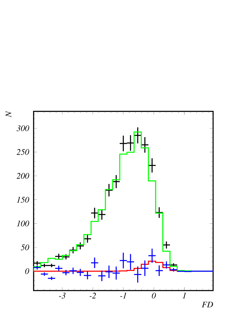
Figure 1.— $FD$ distribution for the region inside $\theta^{2}~{}<~{}0.06$ deg². The black points with error bars are those for the above region, the green histogram is for $\theta^{2}$ inside the (0.1–0.2) [deg²] region, the blue points with error bars are subtracted data using the results of the fit, that is, “gamma-ray–like” events, and the red histogram is the best-fit gamma-ray, i.e., the gamma ray response function.

The best-fit excess was 71$\pm$32 events, where the uncertainty is the 1$\sigma$ statistical error. The gamma-ray response function from the Monte-Carlo simulation is shown by the red histogram. The threshold of this analysis is estimated from the Monte-Carlo simulation to be $\sim$500 GeV. The systematic error on the energy determination is considered to be less than 15%, with the main factor being the uncertainty in the light collection efficiency and atmospheric conditions.

We then made a radial distribution of gamma-ray–like events. $FD$ distributions in various $\theta^{2}$ slices were made. The control background region was again selected in the $\theta^{2}$ range of between 0.1 and 0.2 deg². The standard fitting procedure described above was carried out. The fitted result is shown in Fig. 2.

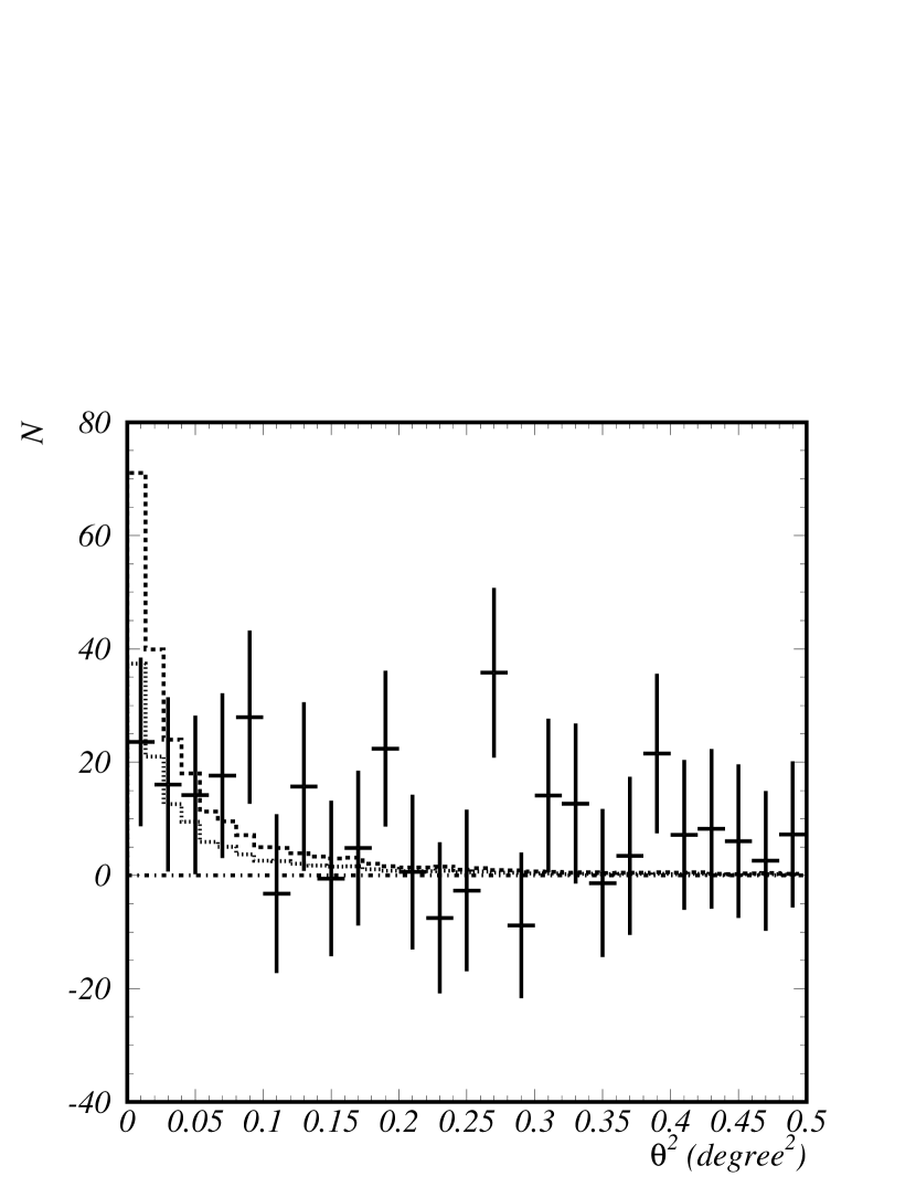
Figure 2.— $\theta^{2}$ plot in the unit of deg². The points with error bars are the result of fit, that is, the “gamma-ray–like” event distribution as a function of $\theta^{2}$. The dot-dashed line is the zero level. The (light) dotted histogram is the best-fit for our point-spread function. The (heavy) dashed histogram is the two-$\sigma$ upper limit for the point-source assumption.

The reduced $\chi^{2}$ for a null assumption (the dot-dashed line) is $\chi^{2}$/DOF = 25.4/25 (where DOF is degrees of freedom). The best fit with the point spread function (PSF) is shown by the dashed histogram, where $\chi^{2}$/D.O.F = 18.1/25. The dashed histogram is the 2$\sigma$ upper limit (135-event excess) for the PSF excess.

In order to examine the morphology, we segmented the field of view into 0.2 $\times$ 0.2 degree² square bins. The $FD$ distributions for corresponding bins were made and fitted. The control-background region is defined as the second-closest layer of 16 bins, all of which are more than 0.3 deg from the center of the target region, i.e., larger than the 0.24 degree point-spread function (PSF). The statistics of the control-background are, therefore, sixteen times larger than that of the signal bin. The results are shown in Fig. 3.

Figure 3.— Significance map. The average telescope pointing position is indicated by the white cross at the center. The dotted-white circle is the point-spread function and the searched region. The dashed-white circle is the fiducial region (1^∘ radius). The thin-white contours are the radio measurement at 4850 MHz (SkyView, 2007) which are well inside the searched region. The color bar indicates the excess in standard deviations over the background (see text for details).

We smoothed the results by averaging the neighboring nine bins. Our sensitivity falls off significantly beyond one degree in radius from the center. The PSF is the 0.24 degree radius circle which fully contains the radio observed SNR (the thin-white contours). According to the Monte-Carlo simulations, 65% of gamma-rays from this SNR should be contained in this circle. The PSF is not a Gaussian and has a broader tail component. In order to contain 90% of events, we need to broaden this cut to 0.5 degree, resulting in a loss of sensitivity. We, therefore, selected the cut at 0.24 degree (1$\sigma$ region). The significance distributions (excess divided by the statistical error before smoothing) are approximately normal (Gaussian) distributions with a mean value of 0.21$\pm$0.13, and a standard deviation of 1.19$\pm$0.12, consistent with null assumption within systematic uncertainties. The statistical significance of the maximum located 0.^∘35 west-north-west from the center is (before smoothing) 3.3$\sigma$, and therefore not compelling.

There is no statistically-significant excess that is consistent with emission from Kepler’s SNR convolved with the telescope PSF. The derived upper limits (ULs) for the gamma-ray flux are shown in Table 1.

Table 1The 2$\sigma$ upper limits to the integral fluxes from Kepler’s SNR at five energy thresholds. The spectral index, $\gamma$, of the energy spectrum (E^-γ) is that used in the Monte-Carlo gamma-ray simulations. Note that the gamma-ray acceptance depends on $\gamma$.

$\gamma$	Threshold [GeV]	Upper Limits [cm-2s-1]
2.1	530	1.7 $\times$ 10-11
2.1	680	1.1 $\times$ 10-11
2.1	930	6.8 $\times$ 10-12
2.1	1300	1.5 $\times$ 10-12
2.1	2400	6.2 $\times$ 10-13
1.9	550	1.7 $\times$ 10-11
1.9	700	1.2 $\times$ 10-11
1.9	930	7.5 $\times$ 10-12
1.9	1300	1.6 $\times$ 10-12
1.9	2400	7.7 $\times$ 10-13
2.3	510	1.8 $\times$ 10-11
2.3	650	1.2 $\times$ 10-11
2.3	930	6.5 $\times$ 10-12
2.3	1200	1.5 $\times$ 10-12
2.3	2300	5.6 $\times$ 10-13

Here, we used a $E^{-2.1\pm 0.2}$ spectrum for the gamma-ray simulation. The ULs range between 10–30% of the Crab nebula flux. The statistically insignificant excess near the center of the field of view, shown in Figs. 1, 2, and 3 only appeared in the lower energy regions. At higher energies, we do not see any excess. Therefore the ULs at lower energies were higher than that at higher energies.

6. Discussion

The upper limits given in Table 1 are plotted on spectral energy distributions in Figs. 4 and 5.

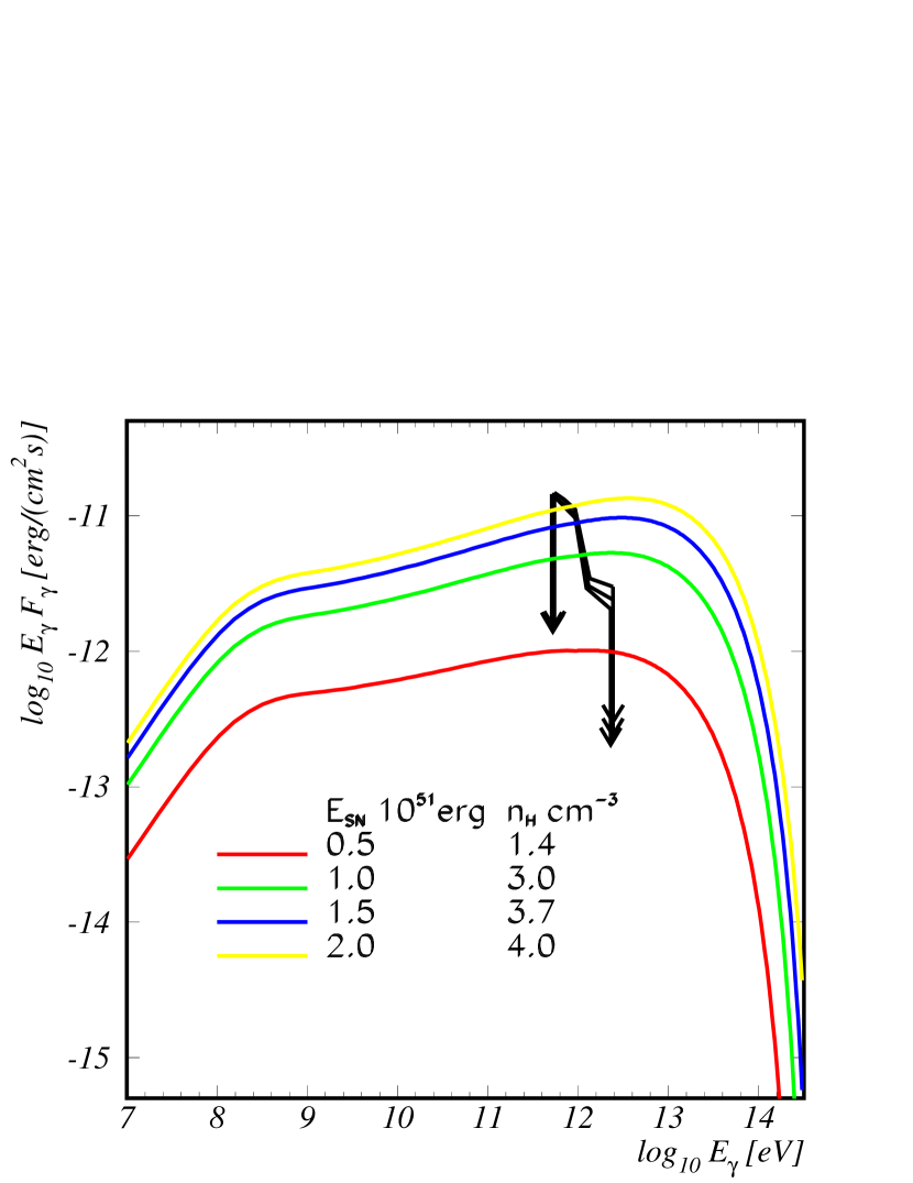
Figure 4.— Spectral energy distributions for a fixed distance of 4.8 kpc. The black curves with arrows at both ends are the upper limits obtained by these observations. Three curves are obtained by different acceptance corrections using three types of energy spectra in the Monte-Carlo simulation (see the caption of Table 1). The colored curves are the theoretical predictions, which are as same as Fig. 3 of Berezhko et al. (2006).

The vertical and horizontal units were fitted to Figs. 3 and 4 in Berezhko et al. (2006) in order to discuss the allowed parameter ranges with respect to our observational upper limits. This theory considered a reasonably wide range of possibilities for the distance of this SNR (3.4–7 kpc) and the supernova explosion energy (0.5–2 $\times$ 10⁵¹ erg). Other adopted parameters, such as the cosmic ray injection rate, expansion rate, and electron-to-proton ratio, while plausible, are open to debate. We do not review those details here but refer readers to the discussion in Berezhko et al. (2006). The black curve with arrows at both ends were obtained from this observation. Three types of the energy spectra ($\propto~{}E^{\gamma}:\gamma=-1.9,~{}-2.1,~{}-2.3$) were used for acceptance correction using the Monte-Carlo simulation. The uncertainty due to the assumption of the energy spectral index is small on a logarithmic scale. The colored curves were obtained from a theoretical prediction by Berezhko et al. (2006). In Fig. 4 the distance to the object was fixed to be 4.8 kpc. The red, green, blue, and yellow curves correspond to different supernova explosion kinetic energies and corresponding number densities of ambient circumstellar material, which came from fitting to the observed shock radius and speed. The most probable is the second one (the green curve) and our upper limits are (in part) below it, meaning that for a distance of 4.8 kpc the explosion energy should be less than $\sim 10^{51}$ erg. Although the green curve is close to a best estimation, a large allowable range of parameter space remains.

Fig. 5 is the case when the supernova explosion energy is fixed at 10⁵¹ erg, and several distances in the allowed range (Reynoso & Goss, 1999) are assumed.

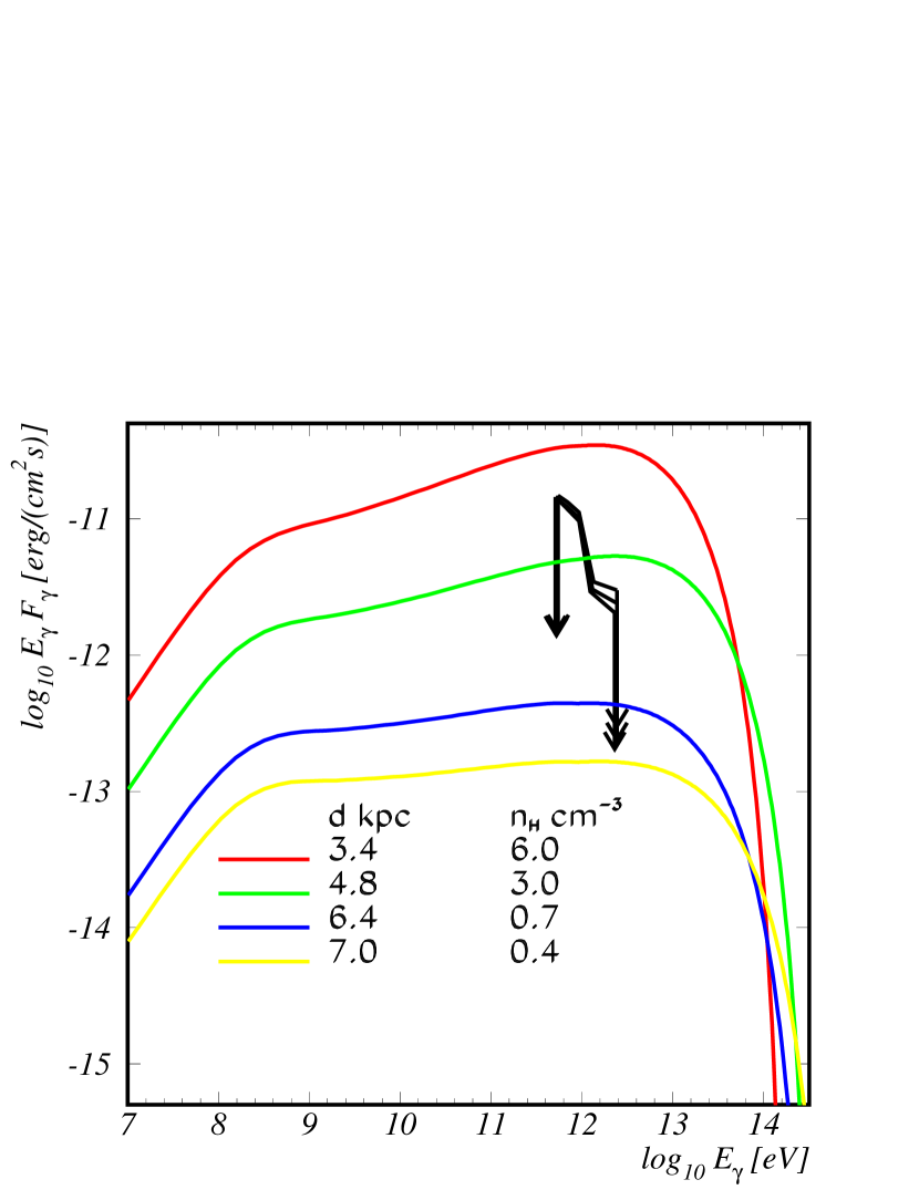
Figure 5.— Spectral energy distributions for a fixed supernova explosion energy of 10⁵¹ erg. The black curve with arrows at both ends are the upper limits obtained by this observation. Three curves are obtained by different acceptance corrections using three types of energy spectra in the Monte-Carlo simulation (Table 1). The colored curves are the theoretical predictions, which are as same as Fig. 4 of Berezhko et al. (2006).

Distances less than $\sim$5 kpc are (for this fixed SN energy) not favored, suggesting that this SNR is marginally more distant than the best current observational estimations. Of course, this conclusion also assumes that all other assumptions in the model are correct, for example, that the expansion is in Sedov phase, that the supernova was Type Ia, that 10% of kinetic energy is transferred to the cosmic-ray energy, etc.

The constraints on the parameters of the distance $d$ and the ambient density $n_{\rm H}$ are illustrated in Fig. 6.

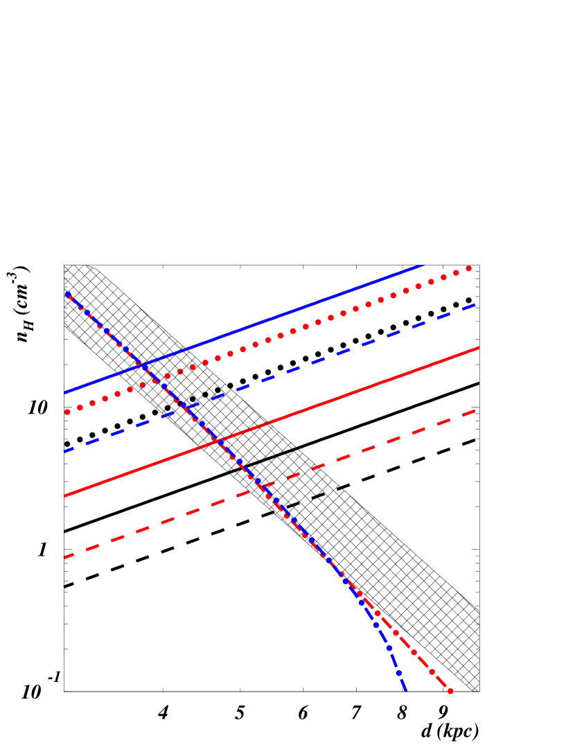
Figure 6.— The allowed region in the plane of the distance ($d$) versus ambient density ($n_{\rm H}$), based on the neutral pion decay $\gamma$-ray emission model where we assume that the total number spectrum of protons is proportional to a power law with an exponential cutoff and the value of the conversion efficiency from the explosion energy to the cosmic-ray energy is 10%. The solid, dashed, and dotted lines indicate the upper limits obtained from the observed 2$\sigma$ upper limits in Table 1, compared with the integral fluxes of the models for the power-law indices 2.1, 1.9, and 2.3, respectively. The colors of the lines represent the cutoff energy of protons; the black, red, and blue ones are obtained with the values $10^{15}$, $10^{14}$, and $10^{13}$ eV, respectively. The allowed regions lie under these upper-limit lines. The hatched region indicates the region which satisfies the Sedov-Taylor solution of the apparent radius of the Kepler’s SNR, 100$"$ at 400 yr with the explosion energy $0.5\sim 2\times 10^{51}$ erg. The dot-dashed lines are obtained from the approximate analytic blast-wave positions of the radius 100$"$, assuming the solution of Truelove & McKee (1999). The red and blue ones are obtained assuming the ejecta power-law index $n=6$ and $n=14$, respectively, with ejecta mass of 1.4$M_{\sun}$ with the explosion energy $10^{51}$ erg.

Here we assume that the total number spectrum of protons is proportional to a power law with an exponential cutoff $E^{-p}\exp(-E/E_{max})$ and that the neutral pion decay $\gamma$-ray emission dominates. If the conversion efficiency ($\epsilon$) from the explosion energy $E_{\rm sn}$ to the cosmic-ray energy is assumed to be 10% (i.e., $\epsilon=0.1$), the normalization factor of the proton spectrum can be determined and the $\gamma$-ray fluxes can be calculated (Mori, 1997) on the assumption of the power-law index $p$ and the cutoff energy $E_{\rm max}$. Given the parameters of the $E_{\rm sn}$, $p$, and $E_{\rm max}$, the upper limits of $n_{\rm H}/d\,^{2}$ are calculated from the observed 2$\sigma$ upper limits in Table 1, compared with the integral fluxes of the model, because the $\gamma$-ray fluxes $F_{\gamma}$ are proportional to $\epsilon E_{\rm sn}n_{\rm H}/d\,^{2}$. In Fig. 6, we plotted the upper limits for the power-law indices 2.1 (solid), 1.9 (dashed), and 2.3 (dotted) and for the cutoff energies of protons $10^{15}$ (black), $10^{14}$ (red), and $10^{13}$ eV (blue). We did not plot the case of $p=2.3$ and $E_{\rm max}=10^{13}$ eV, as the flux in the GeV energy region exceeds the EGRET upper limit.

The apparent radius $\theta$=100$"$ of the Kepler’s SNR at $t_{\rm age}$ gives another constraint. Here we consider two solutions on the expansion law of the blast-wave shock. The first one is the Sedov-Taylor solution : $\theta d\propto(E_{\rm sn}/n_{\rm H})^{1/5}t_{\rm age}^{2/5}$. Another one is the approximate analytic solutions (Truelove & McKee, 1999), which can be applied from the ejecta-dominated phase to the Sedov-Taylor phase. In the latter case, the extra parameters of ejecta mass $M_{\rm ej}$ and the ejecta power-law index $n$, are added to the explosion energy $E_{\rm sn}$ and the ambient matter number density $n_{\rm H}$. The region which is satisfied with the Sedov-Taylor solution of the apparent radius of the Kepler’s SNR, 100$"$ at 400 yr and $E_{\rm sn}=0.5\sim 2\times 10^{51}$ erg are shown as the hatched one in Fig. 6. The dot-dashed lines are obtained from the approximate analytic solution with ejecta mass of 1.4$M_{\sun}$ with the explosion energy $10^{51}$ erg with two kinds of the ejecta power-law index $n=6$ and $n=14$. In the case of $p=2.1$ and $E_{\rm max}=10^{14}$ eV, we note that the CANGAROO-III upper limit implies that the Kepler’s SNR is located at a distance larger than about 4.5 kpc. For the maximum upper limit in the case of $p=2.1$ and $E_{\rm max}=10^{13}$ eV, this means that the SNR is located at a distance larger than about 3.6 kpc.

The distance of a type Ia supernova can be estimated using the correlation between the shape of the optical light curves and the intrinsic luminosity of SNe. Before knowledge of this correlation, Baade (1943) studied the historical light curve of the Kepler’s SN and classified it as a type Ia, and Danziger & Goss (1980) estimated the distance of $3.2\pm 0.7$ kpc using only the maximum luminosity. We can now fit Baade’s data with the improved light-curve template of a type Ia (Jha et al., 2007): $d=4.0\pm 0.4$ kpc on the assumption of a visual extinction $3.27\pm 0.14$ mag (Schaefer, 1996), although the fitted light curve after 100 days is not a good fit.

This value seems to be marginally consistent with our lower limit obtained by this TeV $\gamma$-ray observations. On the other hand, based on the study of H i kinematics and the association of H i cloud with the SNR, Reynoso & Goss (1999) put a lower limit of $d=4.8\pm 1.4$ kpc and an upper limit of 6.4 kpc on the distance. These estimations do not contradict our lower limit.

In any case, a part of the plausible region in parameter space has been rejected, although a large allowed range remains. Although we did not detect any signal in these 15 hours of observations, future detections may strongly constrain the theory. As found in Figs. 3 & 4 in Berezhko et al. (2006), the sensitivity of H.E.S.S. is much lower than the theoretical predictions. The future GLAST mission will also enable the lower energy range to be probed. Future large Cerenkov telescope arrays, such as CTA will allow even more sensitive observations to be made.

7. Conclusion

TeV gamma-ray observations toward the 400 year old remnant of Kepler’s SN were made in 2005 April. Although a measurable flux of TeV-gamma rays had been predicted, we did not observe any statistically significant excess in this region, and the constraints on the allowed parameter range have been discussed. Although a region of parameter range has been rejected, more sensitive measurements are required to constrain the models further.

References

- Aharonian et al. (2001) Aharonian, F., et al. 2001, A&A, 370, 112
- Aharonian et al. (2004) Aharonian, F., et al. 2004, Nature, 432, 75
- Aharonian et al. (2005) Aharonian, F., et al. 2005, ApJ, 437, L7
- Baade (1943) Baade, W. 1943, ApJ, 97, 119
- Berezhko et al. (2006) Berezhko, E. G., Ksenofontov, L. T., & Völk, H. J. 2006, A&A, 452, 217
- Blair (2005) Blair, W. P. 2005, in Supernovae as Cosmological Lighthouses, ASP Conf. Ser., 342, 416
- Daum et al. (1997) Daum, A., et al. 1997, Astropart. Phys., 8, 1
- Danziger & Goss (1980) Danziger, I.J., & Goss, W.M. 1980, MNRAS, 190, 47
- Doggett & Branchi (1985) Doggett, J. B., & Branch, D. 1985, AJ, 90, 2303
- Enomoto et al. (2002a) Enomoto, R., et al. 2002a, Nature, 416, 823
- Enomoto et al. (2002b) Enomoto, R., et al. 2002b, Astropart. Phys., 16, 235
- Enomoto et al. (2006a) Enomoto, R., et al. 2006a, ApJ, 638, 397
- Enomoto et al. (2006b) Enomoto, R., et al. 2006b, ApJ, 652, 1268
- Fisher (1936) Fisher, R. A. 1936, Annals of Eugenics, 7, 179
- Hillas (1985) Hillas, A. M. 1985, Proc. 19th Int. Cosmic Ray Conf. (La Jolla) 3, 445
- Kabuki et al. (2003) Kabuki, S., et al. 2003, Nucl. Instrum. Meth., A500, 318
- Kabuki et al. (2007) Kabuki, S., et al. 2007, ApJ, 668, 968
- Katagiri et al. (2005) Katagiri, H., et al. 2005, ApJ, 619, L163
- Kawachi et al. (2001) Kawachi, A., et al. 2001, Astropart. Phys., 14, 261
- Kinugasa & Tsunemi (2007) Kinugasa, K., & Tsunemi, H. 1999, PASJ, 51, 239
- Mori (1997) Mori, M. 1997, ApJ, 478, 225
- Jha et al. (2007) Jha, S., Riess, A.G., & Kirshner, R.P., ApJ, 659, 122
- Reynolds et al. (2007) Reynolds, S. P., et al. 2007, ApJ, 668, L135
- Reynoso & Goss (1999) Reynoso, E. M., & Goss, W. M. 1999, AJ, 118, 926
- SkyView (2007) NASA, 2007, SkyView (Greenbelt: GFSC), http://skyview.gsfc.nasa.gov
- Nishijima et al. (2005) Nishijima, K., et al. 2005, Proc. 29th Int. Cosmic Ray Conf. (Pune), OG2.7, 101
- Schaefer (1996) Schaefer, B. E. 1996, ApJ, 459, 438
- Truelove & McKee (1999) Truelove, J. K., & McKee, C. F. 1999, ApJS, 120, 299