The plane fixed point problem

Abstract.

In this paper we present proofs of basic results, including those developed so far by H. Bell, for the plane fixed point problem. Some of these results had been announced much earlier by Bell but without accessible proofs. We define the concept of the variation of a map on a simple closed curve and relate it to the index of the map on that curve: Index = Variation + 1. We develop a prime end theory through hyperbolic chords in maximal round balls contained in the complement of a non-separating plane continuum $X$. We define the concept of an outchannel for a fixed point free map which carries the boundary of $X$ minimally into itself and prove that such a map has a unique outchannel, and that outchannel must have variation $=-1$. We also extend Bell’s linchpin theorem for a foliation of a simply connected domain, by closed convex subsets, to arbitrary domains in the sphere.

We introduce the notion of an oriented map of the plane. We show that the perfect oriented maps of the plane coincide with confluent (that is composition of monotone and open) perfect maps of the plane. We obtain a fixed point theorem for positively oriented, perfect maps of the plane. This generalizes results announced by Bell in 1982 (see also [akis99]). It follows that if $X$ is invariant under an oriented map $f$, then $f$ has a point of period at most two in $X$.

1. Introduction

We denote the plane by $\mathbb{C}$, the Riemann sphere by $\mathbb{C}^{\infty}=\mathbb{C}\cup\{\infty\}$, the real line by $\mathbb{R}$ and the unit circle by $S^{1}=\mathbb{R}/\mathbb{Z}$. Let $X$ be a plane continuum. Since $\mathbb{C}$ is locally connected and $X$ is closed, complementary domains of $X$ are open. By $T(X)$ we denote the topological hull of $X$ consisting of $X$ union all of its bounded complementary domains. Thus, $U^{\infty}=\mathbb{C}^{\infty}\setminus T(X)$ is a simply-connected open domain containing $\infty$. The following is a long-standing question in topology.

Fixed Point Question: “Does a continuous function taking a non-separating plane continuum into itself always have a fixed point?”

It is easy to see that a map of a plane continuum to itself can be extended to a perfect map of the plane. We study the slightly more general question, “Is there a plane continuum $Z$ and a perfect continuous function $f:\mathbb{C}\to\mathbb{C}$ taking $Z$ into $T(Z)$ with no fixed points in $T(Z)$?” A Zorn’s Lemma argument shows that if one assumes the answer is “yes,” then there is a subcontinuum $X\subset Z$ minimal with respect to these properties. It will follow from Theorem LABEL:densechannel that for such a minimal continuum, $f(X)=X=\partial T(X)$ (though it may not be the case that $f(T(X))\subset T(X)$). Here $\partial T(X)$ denotes the boundary of $T(X)$. We recover Bell’s result [bell67] (see also Sieklucki [siek68], and Iliadis [ilia70]) that the boundary of $X$ is indecomposable (with a dense channel, explained later).

In this paper we use tools first developed by Bell to elucidate the action of a fixed point free map (should one exist). We are indebted to Bell for sharing his insights with us. Many of the results of this paper were first obtained by him. Unfortunately, many of the proofs were not accessible. We believe that they deserve to be developed in order to be useful to the mathematical community. The results of this paper are also crucial to several recent results regarding the extension of isotopies of plane continua [overtymc07], the existence of fixed points for branched covering maps of the plane [blokoverto1], fixed points in non-invariant plane continua [blokover08a], the existence of locally connected models for all connected Julia sets of complex polynomials [blokover08b] and an estimate on the number of attracting and neutral periodic orbits of complex polynomials [blokoverto2].

We have stated many of these results using existing notions such as prime ends. We introduce Bell’s notion of variation and prove his theorem that index equals variation +1; Theorem 2.13. We also extended Bell’s linchpin Theorem LABEL:Hypmain for simply connected domains to arbitrary domains in the sphere and given a proof using an elegant argument due to Kulkarni and Pinkall [kulkpink94]. Our version of this theorem (Theorem LABEL:KPthrm) is essential for the results later in the paper. Theorem LABEL:outchannel (Unique Outchannel) is a new result due to Bell. Complete proofs of Theorems 2.13, 2.14, LABEL:Hypmain and LABEL:outchannel appear in print for the first time.

The classical fixed point question asks whether each map of a non-separating plane continuum into itself must have a fixed point. Cartwright and Littlewood [cartlitt51] showed that the answer is yes if the map can be extended to an orientation-preserving homeomorphism of the plane. It was 25 years before Bell [bell78] extended this to the class of all homeomorphisms of the plane. Bell announced in 1984 (see also Akis [akis99]) that the Cartwright-Littlewood Theorem can be extended to the class of all holomorphic maps of the plane. These maps behave like orientation-preserving homeomorphisms in the sense that they preserve local orientation. Compositions of open, perfect and of monotone, perfect surjections of the plane are confluent and naturally decompose into two classes, one of which preserves and the other of which reverses local orientation. We show that any confluent map of the plane is itself a composition of a monotone and a light-open map of the plane. We also show that an oriented map of the plane induces a map to the circle of prime ends of an acyclic continuum from the circle of prime ends of a component of its pre-image. Finally we will show that each invariant non-separating plane continuum, under a positively-oriented map of the plane, must contain a fixed point. It follows that any confluent map of the plane has a point of period at most two in any non-separating invariant sub-continuum.

For the convenience of the reader we have included an index at the end of the paper.

2. Tools

Let $p:\mathbb{R}\to S^{1}$ denote the covering map $p(x)=e^{2\pi ix}$. Let $g:S^{1}\to S^{1}$ be a map. By the degree of the map $g$, denoted by $\mathrm{degree}(g)$, we mean the number $\hat{g}(1)-\hat{g}(0)$, where $\hat{g}:\mathbb{R}\to\mathbb{R}$ is a lift of the map $g$ to the universal covering space $\mathbb{R}$ of $S^{1}$ (i.e., $p\circ\hat{g}=g\circ p$). It is well-known that $\mathrm{degree}(g)$ is independent of the choice of the lift.

2.1. Index

Let $g:S^{1}\to\mathbb{C}$ be a map and $f:g(S^{1})\to\mathbb{C}$ a fixed point free map. Define the map $v:S^{1}\to S^{1}$ by

$$v(t)=\frac{f(g(t))-g(t)}{|f(g(t))-g(t)|}.$$

Then the map $v:S^{1}\to S^{1}$ lifts to a map $\widehat{v}:\mathbb{R}\to\mathbb{R}$. Define the index of $f$ with respect to $g$, denoted $\mathrm{ind}(f,g)$ by

$$\mathrm{ind}(f,g)=\widehat{v}(1)-\widehat{v}(0)=\mathrm{degree}(v).$$

Note that $\mathrm{ind}(f,g)$ measures the net number of revolutions of the vector$f(g(t))-g(t)$ as $t$ travels through the unit circle one revolution in the positive direction.

Remark 2.1.

(a) If $g:S^{1}\to\mathbb{C}$ is a constant map with $g(S^{1})=c$ and $f(c)\neq c$, then $\mathrm{ind}(f,g)=0$.
(b)If $f$ is a constant map and $f(\mathbb{C})=w$ with $w\not\in g(S^{1})$, then $\mathrm{ind}(f,g)=\mathrm{win}(g,S^{1},w)$, the winding number of $g$ about $w$. In particular, if $f:S^{1}\to T(S^{1})\setminus S^{1}$ is a constant map, then $\mathrm{ind}(f,id|_{S^{1}})=1$, where $id|_{S^{1}}$ is the identity map on $S^{1}$.

Suppose $S\subset\mathbb{C}$ is a simple closed curve and $A\subset S$ is a subarc of $S$ with endpoints $a$ and $b$. Then we write $A=[a,b]$ if $A$ is the arc obtained by traveling in the counter-clockwise direction from the point $a$ to the point $b$ along $S$. In this case we denote by $<$ the linear order on the arc $A$ such that $a<b$. We will call the order $<$ the counterclockwise order on $A$. Note that $[a,b]\neq[b,a]$.

More generally, for any arc $A=[a,b]\subset S^{1}$, with $a<b$ in the counterclockwise order, define the fractional index [brow90] off$onthesub-path$g—_[a,b]$by$$\mathrm{ind}(f,g|_{[a,b]})=\widehat{v}(b)-\widehat{v}(a).$$While,necessarily,theindexof$f$withrespectto$g$isaninteger,thefractionalindexof$f$on$g—_[a,b]$neednotbe.WeshallhaveoccasiontousefractionalindexintheproofofTheorem~{}\ref{I=V+1}.\par\par\begin{prop}Let$g:S^{1}\to\mathbb{C}$beamapwith$g(S^{1})=S$,andsuppose$f:S\to\mathbb{C}$hasnofixedpointson$S$.Let$a\not=b\in S^{1}$with$[a,b]$denotingthecounterclockwisesubarcon$S^{1}$from$a$to$b$(so$S^{1}=[a,b]\cup[b,a]$).Then$\mathrm{ind}(f,g)=\mathrm{ind}(f,g|_{[a,b]})+\mathrm{ind}(f,g|_{[b,a]})$.\end{prop}\par$

2.2. Stability of Index

The following standard theorems and observations about the stability of index under a fixed point free homotopy are consequences of the fact that index is continuous and integer-valued.

Theorem 2.3.

Let $h_{t}:S^{1}\to\mathbb{C}$ be a homotopy. If $f:\cup_{t\in[0,1]}h_{t}(S^{1})\to\mathbb{C}$ is fixed point free, then $\mathrm{ind}(f,h_{0})=\mathrm{ind}(f,h_{1})$.

An embedding $g:S^{1}\to S\subset\mathbb{C}$ is orientation preserving if $g$ is isotopic to the identity map $id|_{S^{1}}$. It follows from Theorem 2.3 that if $g_{1},g_{2}:S^{1}\to S$ are orientation preserving homeomorphisms and $f:S\to\mathbb{C}$ is a fixed point free map, then $\mathrm{ind}(f,g_{1})=\mathrm{ind}(f,g_{2})$. Hence we can denote $\mathrm{ind}(f,g_{1})$ by $\mathrm{ind}(f,S)$ and if $[a,b]$ is a positively oriented subarc of $S^{1}$ we denote $\mathrm{ind}(f,g_{1}|_{[a,b]})$ by $\mathrm{ind}(f,g_{1}([a,b]))$, by some abuse of notation when the extension of $g_{1}$ over $S^{1}$ is understood.

Theorem 2.4.

Suppose $g:S^{1}\to\mathbb{C}$ is a map with $g(S^{1})=S$, and $f_{1},f_{2}:S\to\mathbb{C}$ are homotopic maps such that each level of the homotopy is fixed point free on $S$. Then $\mathrm{ind}(f_{1},g)=\mathrm{ind}(f_{2},g)$.

In particular, if $S$ is a simple closed curve and $f_{1},f_{2}:S\to\mathbb{C}$ are maps such that there is a homotopy $h_{t}:S\to\mathbb{C}$ from $f_{1}$ to $f_{2}$ with $h_{t}$ fixed point free on $S$ for each $t\in[0,1]$, then $\mathrm{ind}(f_{1},S)=\mathrm{ind}(f_{2},S)$.

Corollary 2.5.

Suppose $g:S^{1}\to\mathbb{C}$ is an orientation preserving embedding with $g(S^{1})=S$, and $f:S\to T(S)$ is a fixed point free map. Then $\mathrm{ind}(f,g)=\mathrm{ind}(f,S)=1$.

Proof.

Since $f(S)\subset T(S)$ which is a disk with boundary $S$ and $f$ has no fixed point on $S$, there is a fixed point free homotopy of $f|_{S}$ to a constant map $c:S\to\mathbb{C}$ taking $S$ to a point in $T(S)\setminus S$. By Theorem 2.4, $\mathrm{ind}(f,g)=\mathrm{ind}(c,g)$. Since $g$ is orientation preserving it follows from Remark 2.1 (b) that $\mathrm{ind}(c,g)=1$. ∎

Theorem 2.6.

Suppose $g:S^{1}\to\mathbb{C}$ is a map with $g(S^{1})=S$, and $f:T(S)\to\mathbb{C}$ is a map such that $\mathrm{ind}(f,g)\not=0$, then $f$ has a fixed point in $T(S)$.

Proof.

Notice that $T(S)$ is a locally connected, non-separating, plane continuum and, hence, contractible. Suppose $f$ has no fixed point in $T(S)$. Choose point $q\in T(S)$. Let $c:S^{1}\to\mathbb{C}$ be the constant map $c(S^{1})=\{q\}$. Let $H$ be a homotopy from $g$ to $c$ with image in $T(S)$. Since $H$ misses the fixed point set of $f$, Theorem 2.3 and Remark 2.1 (a) imply $\mathrm{ind}(f,g)=\mathrm{ind}(f,c)=0$. ∎

2.3. Variation

In this subsection we introduce the notion of variation of a map on an arc and relate it to winding number.

Definition 2.7 (Junctions).

The standard junction $J_{O}$ is the union of the three rays $J^{i}_{O}=\{z\in\mathbb{C}\mid z=re^{i\pi/2},\ r\in[0,\infty)\}$, $J^{+}_{O}=\{z\in\mathbb{C}\mid z=r,\ r\in[0,\infty)\}$, $J^{-}_{O}=\{z\in\mathbb{C}\mid z=re^{i\pi},\ r\in[0,\infty)\}$, having the origin $O$ in common. A junction $J_{v}$ is the image of $J_{O}$ under any orientation-preserving homeomorphism $h:\mathbb{C}\to\mathbb{C}$ where $v=h(O)$. We will often suppress $h$ and refer to $h(J^{i}_{O})$ as $J^{i}_{v}$, and similarly for the remaining rays in $J_{v}$. Moreover, we require that for each neighborhood $W$ of $v$, $d(J^{+}_{v}\setminus W,J^{i}_{v}\setminus W)>0$.

Definition 2.8 (Variation on an arc).

Let $S\subset\mathbb{C}$ be a simple closed curve, $f:S\to\mathbb{C}$ a map and $A=[a,b]$ a subarc of $S$ such that $f(a),f(b)\in T(S)$ and $f(A)\cap A=\emptyset$. We define the variation of $f$ on $A$ with respect to $S$, denoted $\mathrm{var}(f,A,S)$, by the following algorithm:

1. Let $v\in A$ and let $J_{v}$ be a junction with $J_{v}\cap S=\{v\}$.

2. Counting crossings: Consider the set $M=f^{-1}(J_{v})\cap[a,b]$. Each time a point of $f^{-1}(J^{+}_{v})\cap[a,b]$ is immediately followed in $M$, in the counterclockwise order $<$ on $[a,b]\subset S$, by a point of $f^{-1}(J^{i}_{v})$ count $+1$ and each time a point of $f^{-1}(J^{i}_{v})\cap[a,b]$ is immediately followed in $M$ by a point of $f^{-1}(J^{+}_{v})$ count $-1$. Count no other crossings.

3. The sum of the crossings found above is the variation $\mathrm{var}(f,A,S)$.

Note that $f^{-1}(J^{+}_{v})\cap[a,b]$ and $f^{-1}(J^{i}_{v})\cap[a,b]$ are disjoint closed sets in $[a,b]$. Hence, in (2) in the above definition, we count only a finite number of crossings and $\mathrm{var}(f,A,S)$ is an integer. Of course, if $f(A)$ does not meet both $J^{+}_{v}$ and $J^{i}_{v}$, then $\mathrm{var}(f,A,S)=0$.

If $\alpha:S\to\mathbb{C}$ is any map such that $\alpha|_{A}=f|_{A}$ and $\alpha(S\setminus(a,b))\cap J_{v}=\emptyset$, then $\mathrm{var}(f,A,S)=\mathrm{win}(\alpha,S,v)$. In particular, this condition is satisfied if $\alpha(S\setminus(a,b))\subset T(S)\setminus\{v\}$. The invariance of winding number under suitable homotopies implies that the variation $\mathrm{var}(f,A,S)$ also remains invariant under such homotopies. That is, even though the specific crossings in (2) in the algorithm may change, the sum remains invariant. We will state the required results about variation below without proof. Proofs can also be obtained directly by using the fact that $\mathrm{var}(f,A,S)$ is integer-valued and continuous under suitable homotopies.

Proposition 2.9 (Junction Straightening).

Let $S\subset\mathbb{C}$ be a simple closed curve, $f:S\to\mathbb{C}$ a map and $A=[a,b]$ a subarc of $S$ such that $f(a),f(b)\in T(S)$ and $f(A)\cap A=\emptyset$. Any two junctions $J_{v}$ and $J_{u}$ with $u,v\in A$ and $J_{w}\cap S=\{w\}$ for $w\in\{u,v\}$ give the same value for $\mathrm{var}(f,A,S)$. Hence $\mathrm{var}(f,A,S)$ is independent of the particular junction used in Definition 2.8.

The computation of $\mathrm{var}(f,A,S)$ depends only upon the crossings of the junction $J_{v}$ coming from a proper compact subarc of the open arc $(a,b)$. Consequently, $\mathrm{var}(f,A,S)$ remains invariant under homotopies $h_{t}$ of $f|_{[a,b]}$ in the complement of $\{v\}$ such that $h_{t}(a),h_{t}(b)\not\in J_{v}$ for all $t$. Moreover, the computation is stable under an isotopy $h_{t}$ of the plane that moves the entire junction $J_{v}$ (even off $A$), provided in the isotopy $h_{t}(v)\not\in f(A)$ and $f(a),f(b)\not\in h_{t}(J_{v})$ for all $t$.

In case $A$ is an open arc $(a,b)\subset S$ such that $\mathrm{var}(f,\overline{A},S)$ is defined, it will be convenient to denote $\mathrm{var}(f,\overline{A},S)$ by $\mathrm{var}(f,A,S)$

The following Lemma follows immediately from the definition.

Lemma 2.10.

Let $S\subset\mathbb{C}$ be a simple closed curve. Suppose that $a<c<b$ are three points in $S$ such that $\{f(a),f(b),f(c)\}\subset T(S)$ and $f([a,b])\cap[a,b]=\emptyset$. Then $\mathrm{var}(f,[a,b],S)=\mathrm{var}(f,[a,c],S)+\mathrm{var}(f,[c,b],S)$.

Definition 2.11 (Variation on a finite union of arcs).

Let $S\subset\mathbb{C}$ be a simple closed curve and $A=[a,b]$ a subcontinuum of $S$ with partition a finite set $F=\{a=a_{0}<a_{1}<\dots<a_{n}=b\}$. For each $i$ let $A_{i}=[a_{i},a_{i+1}]$. Suppose that $f$ satisfies $f(a_{i})\in T(S)$ and $f(A_{i})\cap A_{i}=\emptyset$ for each $i$. We define the variation of $f$ on $A$ with respect to $S$, denoted $\mathrm{var}(f,A,S)$, by var(f,A,S)=∑_i=0^n-1 var(f,[a_i,a_i+1],S). In particular, we include the possibility that $a_{n}=a_{0}$ in which case $A=S$.

By considering a common refinement of two partitions $F_{1}$ and $F_{2}$ of an arc $A\subset S$ such that $f(F_{1})\cup f(F_{2})\subset T(S)$ and satisfying the conditions in Definition 2.11, it follows from Lemma 2.10 that we get the same value for $\mathrm{var}(f,A,S)$ whether we use the partition $F_{1}$ or the partition $F_{2}$. Hence, $\mathrm{var}(f,A,S)$ is well-defined. If $A=S$ we denote $\mathrm{var}(f,S,S)$ simply by $\mathrm{var}(f,S)$.

2.4. Index and variation for finite partitions

What links Theorem 2.6 with variation is Theorem 2.13 below, first announced by Bell in the mid 1980’s (see also Akis [akis99]). Our proof is a modification of Bell’s unpublished proof. We first need a variant of Proposition 2.9. Let $r:\mathbb{C}\to T(S^{1})$ be radial retraction: $r(z)=\frac{z}{|z|}$ when $|z|\geq 1$ and $r|_{T(S^{1})}=id|_{T(S^{1})}$.

Lemma 2.12 (Curve Straightening).

Suppose $f:S^{1}\to\mathbb{C}$ is a map with no fixed points on $S^{1}$. If $[a,b]\subset S^{1}$ is a proper subarc with $f([a,b])\cap[a,b]=\emptyset$, $f((a,b))\subset\mathbb{C}\setminus T(S^{1})$ and $f(\{a,b\})\subset S^{1}$, then there exists a map $\tilde{f}:S^{1}\to\mathbb{C}$ such that $\tilde{f}|_{S^{1}\setminus(a,b)}=f|_{S^{1}\setminus(a,b)}$, $\tilde{f}|_{[a,b]}:[a,b]\to(\mathbb{C}\setminus T(S^{1}))\cup\{f(a),f(b)\}$ and $\tilde{f}|_{[a,b]}$ is homotopic to $f|_{[a,b]}$ in $\{a,b\}\cup\mathbb{C}\setminus T(S)$ relative to $\{a,b\}$, so that $r|_{\tilde{f}([a,b])}$ is locally one-to-one. Moreover, $\mathrm{var}(f,[a,b],S^{1})=\mathrm{var}(\tilde{f},[a,b],S^{1})$.

Note that if $\mathrm{var}(f,[a,b],S^{1})=0$, then $r$ carries $\tilde{f}([a,b])$ one-to-one onto the arc (or point) in $S^{1}\setminus(a,b)$ from $f(a)$ to $f(b)$. If the $\mathrm{var}(f,[a,b],S^{1})=m>0$, then $r\circ\tilde{f}$ wraps the arc $[a,b]$ counterclockwise about $S^{1}$ so that $\tilde{f}([a,b])$ meets each ray in $J_{v}$ $m$ times. A similar statement holds for negative variation. Note also that it is possible for index to be defined yet variation not to be defined on a simple closed curve $S$. For example, consider the map $z\to 2z$ with $S$ the unit circle since there is no partition of $S$ satisfying the conditions in Definition 2.8.

Theorem 2.13 (Index = Variation + 1, Bell).

Suppose $g:S^{1}\to\mathbb{C}$ is an orientation preserving embedding onto a simple closed curve $S$ and $f:S\to\mathbb{C}$ is a fixed point free map. If $F=\{a_{0}<a_{1}<\dots<a_{n}\}$ is a partition of $S$ and $A_{i}=[a_{i},a_{i+1}]$ for $i=0,1,\dots,n$ with $a_{n+1}=a_{0}$ such that $f(F)\subset T(S)$ and $f(A_{i})\cap A_{i}=\emptyset$ for each $i$, then ind(f,S)=ind(f,g)=∑_i=0^nvar(f,A_i,S)+1=var(f,S)+1.

Proof.

By an appropriate conjugation of $f$ and $g$, we may assume without loss of generality that $S=S^{1}$ and $g=id$. Let $F$ and $A_{i}=[a_{i},a_{i+1}]$ be as in the hypothesis. Consider the collection of arcs K={K⊂S∣$K$ is the closure of a component of $S\cap f^{-1}(f(S)\setminus T(S))$}. For each $K\in\mathcal{K}$, there is an $i$ such that $K\subset A_{i}$. Since $f(A_{i})\cap A_{i}=\emptyset$, it follows from the remark after Definition 2.8 that $\mathrm{var}(f,A_{i},S)=\sum_{K\subset A_{i},K\in\mathcal{K}}\mathrm{var}(f,K,S)$. By the remark following Proposition 2.9, we can compute $\mathrm{var}(f,K,S)$ using one fixed junction for $A_{i}$. It is now clear that there are at most finitely many $K\in\mathcal{K}$ with $\mathrm{var}(f,K,S)\not=0$. Moreover, the images of the endpoints of each $K$ lie on $S$.

Let $m$ be the cardinality of the set $\mathcal{K}_{f}=\{K\in\mathcal{K}\mid\mathrm{var}(f,K,S)\not=0\}$. By the above remarks, $m<\infty$ and $\mathcal{K}_{f}$ is independent of the partition $F$. We prove the theorem by induction on $m$.

Suppose for a given $f$ we have $m=0$. Observe that from the definition of variation and the fact that the computation of variation is independent of the choice of an appropriate partition, it follows that, var(f,S)=∑_K∈K var(f,K,S)=0.

We claim that there is a map $f_{1}:S\to\mathbb{C}$ with $f_{1}(S)\subset T(S)$ and a homotopy $H$ from $f|_{S}$ to $f_{1}$ such that each level $H_{t}$ of the homotopy is fixed point free and $\mathrm{ind}(f_{1},id|_{S})=1$.

To see the claim, first apply the Curve Straightening Lemma 2.12 to each $K\in\mathcal{K}$ (if there are infinitely many, they form a null sequence) to obtain a fixed point free homotopy of $f|_{S}$ to a map $\tilde{f}:S\to\mathbb{C}$ such that $r|_{\tilde{f}(K)}$ is locally one-to-one on each $K\in\mathcal{K}$, where $r$ is radial retraction of $\mathbb{C}$ to $T(S)$, and $\mathrm{var}(\tilde{f},K,S)=0$ for each $K\in\mathcal{K}$. Let $K$ be in $\mathcal{K}$ with endpoints $x,y$. Since $\tilde{f}(K)\cap K=\emptyset$ and $\mathrm{var}(\tilde{f},K,S)=0$, $r|_{\tilde{f}(K)}$ is one-to-one, and $r\circ\tilde{f}(K)\cap K=0$. Define $f_{1}|_{K}=r\circ\tilde{f}|_{K}$. Then $f_{1}|_{K}$ is fixed point free homotopic to $f|_{K}$ (with endpoints of $K$ fixed). Hence, if $K\in\mathcal{K}$ has endpoints $x$ and $y$, then $f_{1}$ maps $K$ to the subarc of $S$ with endpoints $f(x)$ and $f(y)$ such that $K\cap f_{1}(K)=\emptyset$. Since $\mathcal{K}$ is a null family, we can do this for each $K\in\mathcal{K}$ and set $f_{1}|_{S^{1}\setminus\cup\mathcal{K}}=f|_{S^{1}\setminus\cup\mathcal{K}}$ so that we obtain the desired $f_{1}:S\to\mathbb{C}$ as the end map of a fixed point free homotopy from $f$ to $f_{1}$. Since $f_{1}$ carries $S$ into $T(S)$, Corollary 2.5 implies $\mathrm{ind}(f_{1},id|_{S})=1$.

Since the homotopy $f\simeq f_{1}$ is fixed point free, it follows from Theorem 2.4 that $\mathrm{ind}(f,id|_{S})=1$. Hence, the theorem holds if $m=0$ for any $f$ and any appropriate partition $F$.

By way of contradiction suppose the collection $\mathcal{F}$ of all maps $f$ on $S^{1}$ which satisfy the hypotheses of the theorem, but not the conclusion is non-empty. By the above $0<|\mathcal{K}_{f}|<\infty$ for each. Let $f\in\mathcal{F}$ be a counterexample for which $m=|\mathcal{K}_{f}|$ is minimal. By modifying $f$, we will show there exists $f_{1}\in\mathcal{F}$ with $|\mathcal{K}_{f_{1}}|<m$, a contradiction.

Choose $K\in\mathcal{K}$ such that $\mathrm{var}(f,K,S)\not=0$. Then $K=[x,y]\subset A_{i}=[a_{i},a_{i+1}]$ for some $i$. By the Curve Straightening Lemma 2.12 and Theorem 2.4, we may suppose $r|_{f(K)}$ is locally one-to-one on $K$. Define a new map $f_{1}:S\to\mathbb{C}$ by setting $f_{1}|_{\overline{S\setminus K}}=f|_{\overline{S\setminus K}}$ and setting $f_{1}|_{K}$ equal to the linear map taking $[x,y]$ to the subarc $f(x)$ to $f(y)$ on $S$ missing $[x,y]$. Figure 1 (left) shows an example of a (straightened) $f$ restricted to $K$ and the corresponding $f_{1}$ restricted to $K$ for a case where $\mathrm{var}(f,K,S)=1$, while Figure 1 (right) shows a case where $\mathrm{var}(f,K,S)=-2$.

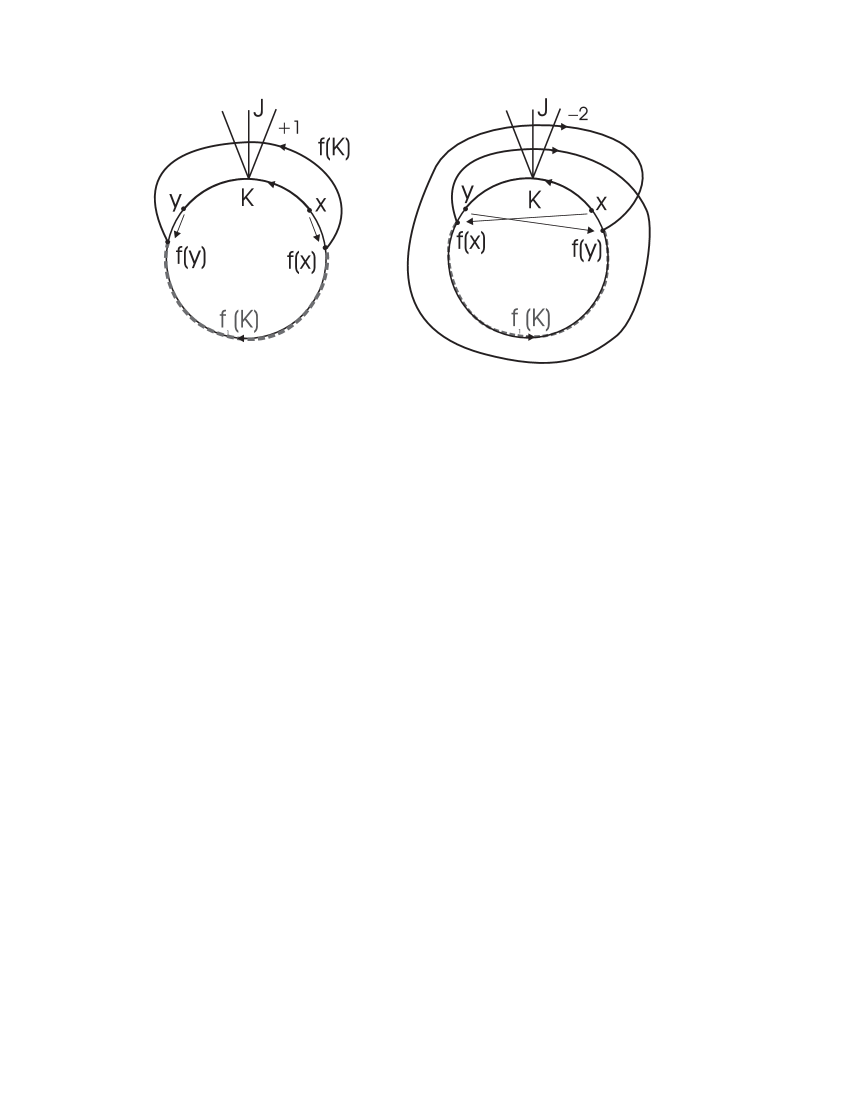
Figure 1. Replacing $f:S\to\mathbb{C}$ by $f_{1}:S\to\mathbb{C}$ with one less subarc of nonzero variation.

Since on $\overline{S\setminus K}$, $f$ and $f_{1}$ are the same map, we have var(f,S∖K,S)=var(f_1,S∖K,S). Likewise for the fractional index, ind(f,S∖K)=ind(f_1,S∖K). By definition (refer to the observation we made in the case $m=0$), var(f,S)=var(f,S∖K,S)+var(f,K,S) var(f_1,S)=var(f_1,S∖K,S)+var(f_1,K,S) and by Proposition 2.2, ind(f,S)=ind(f,S∖K)+ind(f,K) ind(f_1,S)=ind(f_1,S∖K)+ind(f_1,K). Consequently, var(f,S)-var(f_1,S)=var(f,K,S)-var(f_1,K,S) and ind(f,S)-ind(f_1,S)=ind(f,K)-ind(f_1,K).

We will now show that the changes in index and variation, going from $f$ to $f_{1}$ are the same (i.e., we will show that $\mathrm{var}(f,K,S)-\mathrm{var}(f_{1},K,S)=\mathrm{ind}(f,K)-\mathrm{ind}(f_{1},K)$). We suppose first that $\mathrm{ind}(f,K)=n+\alpha$ for some nonnegative $n\in\mathbb{N}$ and $0\leq\alpha<1$. That is, the vector $f(z)-z$ turns through $n$ full revolutions counterclockwise and $\alpha$ part of a revolution counterclockwise as $z$ goes from $x$ to $y$ counterclockwise along $S$. (See Figure 1 (left) for a case $n=0$ and $\alpha$ about $0.8$.) Then as $z$ goes from $x$ to $y$ counterclockwise along $S$, $f_{1}(z)$ goes along $S$ from $f(x)$ to $f(y)$ in the clockwise direction, so $f_{1}(z)-z$ turns through $-(1-\alpha)=\alpha-1$ part of a revolution. Hence, $\mathrm{ind}(f_{1},K)=\alpha-1$. It is easy to see that $\mathrm{var}(f,K,S)=n+1$ and $\mathrm{var}(f_{1},K,S)=0$. Consequently, var(f,K,S)-var(f_1,K,S)=n+1-0=n+1 and ind(f,K)-ind(f_1,K)=n+α-(α-1)=n+1.

In Figure 1 on the left we assumed that $f(x)<x<y<f(y)$. The cases where $f(y)<x<y<f(x)$ and $f(x)=f(y)$ are treated similarly. In this case $f_{1}$ still wraps around in the positive direction, but the computations are slightly different: $\mathrm{var}(f,K)=1$, $\mathrm{ind}(f,K)=1+\alpha$, $\mathrm{var}(f_{1},K)=0$ and $\mathrm{ind}(f_{1},K)=\alpha$.

Thus when $n\geq 0$, in going from $f$ to $f_{1}$, the change in variation and the change in index are the same. However, in obtaining $f_{1}$ we have removed one $K\in\mathcal{K}_{f}$, reducing the minimal $m=|\mathcal{K}_{f}|$ for $f$ by one, producing a counterexample $f_{1}$ with $|\mathcal{K}_{f_{1}}|=m-1$, a contradiction.

The cases where $\mathrm{ind}(f,K)=n+\alpha$ for negative $n$ and $0<\alpha<1$ are handled similarly, and illustrated for $n=-2$ and $\alpha$ about $0.4$ in Figure 1 (right).

∎

2.5. Locating arcs of negative variation

The principal tool in proving Theorem LABEL:outchannel (unique outchannel) is the following theorem first obtained by Bell (unpublished). It provides a method for locating arcs of negative variation on a curve of index zero.

Theorem 2.14 (Lollipop Lemma, Bell).

Let $S\subset\mathbb{C}$ be a simple closed curve and $f:T(S)\to\mathbb{C}$ a fixed point free map. Suppose $F=\{a_{0}<\dots<a_{n}<a_{n+1}<\dots<a_{m}\}$ is a partition of $S$, $a_{m+1}=a_{0}$ and $A_{i}=[a_{i},a_{i+1}]$ such that $f(F)\subset T(S)$ and $f(A_{i})\cap A_{i}=\emptyset$ for $i=0,\dots,m$. Suppose $I$ is an arc in $T(S)$ meeting $S$ only at its endpoints $a_{0}$ and $a_{n+1}$. Let $J_{a_{0}}$ be a junction in $(\mathbb{C}\setminus T(S))\cup\{a_{0}\}$ and suppose that $f(I)\cap(I\cup J_{a_{0}})=\emptyset$. Let $R=T([a_{0},a_{n+1}]\cup I)$ and $L=T([a_{n+1},a_{m+1}]\cup I)$. Then one of the following holds:

1. If $f(a_{n+1})\in R$, then ∑_i≤nvar(f,A_i,S)+1=ind(f,I∪[a_0,a_n+1]) .

2. If $f(a_{n+1})\in L$, then ∑_i¿nvar(f,A_i,S)+1=ind(f,I∪[a_n+1,a_m+1]).

(Note that in (1) in effect we compute $\mathrm{var}(f,\partial R)$ but technically, we have not defined $\mathrm{var}(f,A_{i},\partial R)$ since the endpoints of $A_{i}$ do not have to map inside $R$ but they do map into $T(S)$. Similarly in Case (2).)

Proof.

Without loss of generality, suppose $f(a_{n+1})\in L$. Let $C=[a_{n+1},a_{m+1}]\cup I$ (so $T(C)=L$). We want to construct a map $f^{\prime}:C\to\mathbb{C}$, fixed point free homotopic to $f|_{C}$, that does not change variation on any arc $A_{i}$ in $C$ and has the properties listed below.

1. $f^{\prime}(a_{i})\in L$ for all $n+1\leq i\leq m+1$. Hence $\mathrm{var}(f^{\prime},A_{i},C)$ is defined for each $i>n$.

2. $\mathrm{var}(f^{\prime},A_{i},C)=\mathrm{var}(f,A_{i},S)$ for all $n+1\leq i\leq m$.

3. $\mathrm{var}(f^{\prime},I,C)=\mathrm{var}(f,I,S)=0$.

4. $\mathrm{ind}(f^{\prime},C)=\mathrm{ind}(f,C)$.

Having such a map, it then follows from Theorem 2.13, that ind(f’,C)=∑_i=n+1^m var(f’,A_i,C)+var(f’,I,C)+1.

By Theorem 2.4 $\mathrm{ind}(f^{\prime},C)=\mathrm{ind}(f,C)$. By (2) and (3), $\sum_{i>n}\mathrm{var}(f^{\prime},A_{i},C)+\mathrm{var}(f^{\prime},I,C)=\sum_{i>n}\mathrm{var}(f,A_{i},S)$ and the Theorem would follow.

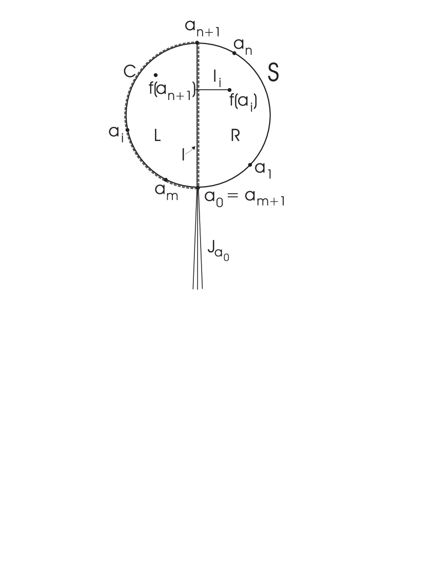
Figure 2. Bell’s Lollipop.

It remains to define the map $f^{\prime}:C\to\mathbb{C}$ with the above properties. For each $i$ such that $n+1\leq i\leq m+1$, chose an arc $I_{i}$ joining $f(a_{i})$ to $L$ as follows:

1. If $f(a_{i})\in L$, let $I_{i}$ be the degenerate arc $\{f(a_{i})\}$.

2. If $f(a_{i})\in R$ and $n+1<i<m+1$, let $I_{i}$ be an arc in $R\setminus\{a_{0},a_{n+1}\}$ joining $f(a_{i})$ to $I$.

3. If $f(a_{0})\in R$, let $I_{0}$ be an arc joining $f(a_{0})$ to $L$ such that $I_{0}\cap(L\cup J_{a_{0}})\subset A_{n+1}\setminus\{a_{n+1}\}$.

Let $x_{n+1}=y_{n+1}=a_{n+1}$, $y_{0}=y_{m+1}\in I\setminus\{a_{0},a_{n+1}\}$ and $x_{0}=x_{m+1}\in A_{m}\setminus\{a_{m},a_{m+1}\}$. For $n+1<i<m+1$, let $x_{i}\in A_{i-1}$ and $y_{i}\in A_{i}$ such that $y_{i-1}<x_{i}<a_{i}<y_{i}<x_{i+1}$. For $n+1<i<m+1$ let $f^{\prime}(a_{i})$ be the endpoint of $I_{i}$ in $L$, $f^{\prime}(x_{i})=f^{\prime}(y_{i})=f(a_{i})$ and extend $f^{\prime}$ continuously from $[x_{i},a_{i}]\cup[a_{i},y_{i}]$ onto $I_{i}$ and define $f^{\prime}$ from $[y_{i},x_{i+1}]\subset A_{i}$ onto $f(A_{i})$ by $f^{\prime}|_{[y_{i},x_{i+1}]}=f\circ h_{i}$, where $h_{i}:[y_{i},x_{i+1}]\to A_{i}$ is a homeomorphism such that $h_{i}(y_{i})=a_{i}$ and $h_{i}(x_{i+1})=a_{i+1}$. Similarly, define $f^{\prime}$ on $[y_{0},a_{n+1}]\subset I$ to $f(I)$ by $f|_{[y_{0},a_{n+1}]}=f\circ h_{0}$, where $h_{0}:[y_{0},a_{n+1}]\to I$ is an onto homeomorphism such that $h(a_{n+1})=a_{n+1}$ and extend $f^{\prime}$ from $[x_{m+1},a_{0}]\subset A_{m}$ and $[a_{o},y_{0}]\subset I$ onto $I_{0}$ such that $f^{\prime}(x_{m+1})=f^{\prime}(y_{0})=f(a_{0})$ and $f^{\prime}(a_{0})$ is the endpoint of $I_{0}$ in $L$.

Note that $f^{\prime}(A_{i})\cap A_{i}=\emptyset$ for $i=n+1,\dots,m$ and $f^{\prime}(I)\cap[I\cup J_{a_{0}}]=\emptyset$. To compute the variation of $f^{\prime}$ on each of $A_{m}$ and $I$ we can use the junction $J_{a_{0}}$ Hence $\mathrm{var}(f^{\prime},I,C)=0$ and, by the definition of $f^{\prime}$ on $A_{m}$, $\mathrm{var}(f^{\prime},A_{m},C)=\mathrm{var}(f,A_{m},S)$. For $i=n+1,\dots,m-1$ we can use the same junction $J_{v_{i}}$ to compute $\mathrm{var}(f^{\prime},A_{i},C)$ as we did to compute $\mathrm{var}(f,A_{i},S)$. Since $I_{i}\cup I_{i+1}\subset T(S)\setminus A_{i}$ we have that $f^{\prime}([a_{i},y_{i}])\cup f^{\prime}([x_{i+1},a_{i+1}])\subset I_{i}\cup I_{i+1}$ misses that junction and, hence, make no contribution to variation $\mathrm{var}(f^{\prime},A_{i},C)$. Since $f^{\prime-1}(J_{v_{i}})\cap[y_{i},x_{i+1}]$ is isomorphic to $f^{-1}(J_{v_{i}})\cap A_{i}$, $\mathrm{var}(f^{\prime},A_{i},C)=\mathrm{var}(f,A_{i},S)$ for $i=n+1,\dots,m$.

To see that $f^{\prime}$ is fixed point free homotopic to $f|_{C}$, note that we can pull the image of $A_{i}$ back along the arcs $I_{i}$ and $I_{i+1}$ in $R$ without fixing a point of $A_{i}$ at any level of the homotopy. Since $f^{\prime}$ and $f|_{C}$ are fixed point free homotopic and $f$ has no fixed points in $T(S)$, it follows from Theorems 2.4 and 2.6, that $\mathrm{ind}(f^{\prime},C)=\mathrm{ind}(f,C)=0$. ∎

Note that if $f$ is fixed point free on $T(S)$, then $\mathrm{ind}(f,S)=0$ and the next Corollary follows.

Corollary 2.15.

Assume the hypotheses of Theorem 2.14. Suppose, in addition, $f$ is fixed point free on $T(S)$. Then if $f(a_{n+1})\in R$ there exists $i\leq n$ such that $\mathrm{var}(f,A_{i},S)<0$. If $f(a_{n+1})\in L$ there exists $i>n$ such that $\mathrm{var}(f,A_{i},S)<0$.

2.6. Crosscuts and bumping arcs

For the remainder of Section 2, our Standing Hypotheses are that $f:\mathbb{C}\to\mathbb{C}$ takes continuum $X$ into $T(X)$ with no fixed points in $T(X)$, and $X$ is minimal with respect to these properties.

Definition 2.16 (Bumping Simple Closed Curve).

A simple closed curve $S$ in $\mathbb{C}$ which has the property that $S\cap X$ is nondegenerate and $T(X)\subset T(S)$ is said to be a bumping simple closed curve for $X$. A subarc $A$ of a bumping simple closed curve, whose endpoints lie in $X$, is said to be a bumping (sub)arc for $X$. Moreover, if $S^{\prime}$ is any bumping simple closed curve for $X$ which contains $A$, then $S^{\prime}$ is said to complete $A$.

A crosscut of $U^{\infty}=\mathbb{C}^{\infty}\setminus T(X)$ is an open arc $Q$ lying in $U^{\infty}$ such that $\overline{Q}$ is an arc with endpoints $a\not=b\in T(X)$. In this case we will often write $Q=(a,b)$. (As seems to be traditional, we use “crosscut of $T(X)$” interchangeably with “crosscut of $U^{\infty}$.”) If $S$ is a bumping simple closed curve so that $X\cap S$ is nondegenerate, then each component of $S\setminus X$ is a crosscut of $T(X)$. A similar statement holds for a bumping arc $A$. Given a non-separating continuum $T(X)$, let $A\subset\mathbb{C}$ be a crosscut of $U^{\infty}=\mathbb{C}^{\infty}\setminus T(X)$. Given a crosscut $A$ of $U^{\infty}$ denote by $\mathrm{Sh}(A)$, the shadow of $A$, the bounded component of $\mathbb{C}\setminus[T(X)\cup A]$.

Since $f$ has no fixed points in $T(X)$ and $X$ is compact, we can choose a bumping simple closed curve $S$ in a small neighborhood of $T(X)$ such that all crosscuts in $S\setminus X$ are small, have positive distance to their image and so that $f$ has no fixed points in $T(S)$. Thus, we obtain the following corollary to Theorem 2.6.

Corollary 2.17.

There is a bumping simple closed curve $S$ for $X$ such that $f|_{T(S)}$ is fixed point free; hence, by 2.6, $\mathrm{ind}(f,S)=0$. Moreover, any bumping simple closed curve $S^{\prime}$ for $X$ such that $S^{\prime}\subset T(S)$ has $\mathrm{ind}(f,S^{\prime})=0$. Furthermore, any crosscut $Q$ of $T(X)$ for which $f$ has no fixed points in $T(X\cup Q)$ can be completed to a bumping simple closed curve $S$ for $X$ for which $\mathrm{ind}(f,S)=0$.

Proposition 2.18.

Suppose $A$ is a bumping subarc for $X$. If $\mathrm{var}(f,A,S)$ is defined for some bumping simple closed curve $S$ completing $A$, then for any bumping simple closed curve $S^{\prime}$ completing $A$, $\mathrm{var}(f,A,S)=\mathrm{var}(f,A,S^{\prime})$.

Proof.

Since $\mathrm{var}(f,A,S)$ is defined, $A=\cup_{i=1}^{n}A_{i}$, where each $A_{i}$ is a bumping arc with $A_{i}\cap f(A_{i})=\emptyset$ and $|A_{i}\cap A_{j}|\leq 1$ if $i\neq j$. By the remark following Definition 2.11, it suffices to assume that $A\cap f(A)=\emptyset$. Let $S$ and $S^{\prime}$ be two bumping simple closed curves completing $A$ for which variation is defined. Let $J_{a}$ and $J_{a^{\prime}}$ be junctions whereby $\mathrm{var}(f,A.S)$ and $\mathrm{var}(f,A,S^{\prime})$ are respectively computed. Suppose first that both junctions lie (except for $\{a,a^{\prime}\}$) in $\mathbb{C}\setminus(T(S)\cup T(S^{\prime}))$. By the Junction Straightening Proposition 2.9, either junction can be used to compute either variation on $A$, so the result follows. Otherwise, at least one junction is not in $\mathbb{C}\setminus(T(S)\cup T(S^{\prime}))$. But both junctions are in $\mathbb{C}\setminus T(X\cup A)$. Hence, we can find another bumping simple closed curve $S^{\prime\prime}$ such that $S^{\prime\prime}$ completes $A$, and both junctions lie in $(\mathbb{C}\setminus T(S^{\prime\prime}))\cup\{a,a^{\prime}\}$. Then by the Propositions 2.9 and the definition of variation, $\mathrm{var}(f,A,S)=\mathrm{var}(f,A,S^{\prime\prime})=\mathrm{var}(f,A,S^{\prime})$. ∎

It follows from Proposition 2.18 that variation on a crosscut $Q$, with $\overline{Q}\cap f(\overline{Q})=\emptyset$, of $T(X)$ is independent of the bumping simple closed curve $S$ for $T(X)$ of which $Q$ is a subarc and is such that $\mathrm{var}(f,S)$ is defined. Hence, given a bumping arc $A$ of $X$, we can denote $\mathrm{var}(f,A,S)$ simply by $\mathrm{var}(f,A)$ when $X$ is understood.

The following proposition follows from Corollary 2.17, Proposition 2.18 and Theorem 2.13.

Proposition 2.19.

Suppose $Q$ is a crosscut of $T(X)$ such that $f$ is fixed point free on $T(X\cup Q)$ and $f(\overline{Q})\cap\overline{Q}=\emptyset$. Suppose $Q$ is replaced by a bumping subarc $A$ with the same endpoints such that $Q\cup T(X)$ separates $A\setminus X$ from $\infty$ and each component $Q_{i}$ of $A\setminus X$ is a crosscut such that $f(\overline{Q_{i}})\cap\overline{Q_{i}}=\emptyset$. Then var(f,Q,X)=∑_i var(f,Q_i,X)=var(f,A,X).

2.7. Index and Variation for Carathéodory Loops

We extend the definitions of index and variation to Carathéodory loops.

Definition 2.20 (Carathéodory Loop).

Let $g:S^{1}\to\mathbb{C}$ such that $g$ is continuous and has a continuous extension $\psi:\overline{\mathbb{C}^{\infty}\setminus T(S^{1})}\to\overline{\mathbb{C}^{\infty}\setminus T(g(S^{1}))}$ such that $\psi|_{\mathbb{C}\setminus T(S^{1})}$ is an orientation preserving homeomorphism from $\mathbb{C}\setminus T(S^{1})$ onto $\mathbb{C}\setminus T(g(S^{1}))$. We call $g$ (and loosely, $S=g(S^{1})$), a Carathéodory loop.

In particular, if $g:S^{1}\to g(S^{1})=S$ is a continuous extension of a Riemann map $\psi:\Delta^{\infty}\to\mathbb{C}^{\infty}\setminus T(g(S^{1}))$, then $g$ is a Carathéodory loop, where $\Delta^{\infty}=\{z\in\mathbb{C}^{\infty}\mid|z|>1\}$ is the “unit disk” about $\infty$.

Let $g:S^{1}\to\mathbb{C}$ be a Carathéodory loop and let $f:g(S^{1})\to\mathbb{C}$ be a fixed point free map. In order to define variation of $f$ on $g(S^{1})$, we do the partitioning in $S^{1}$ and transport it to the Carathéodory loop $S=g(S^{1})$. An allowable partition of $S^{1}$ is a set $\{a_{0}<a_{1}<\dots<a_{n}\}$ in $S^{1}$ ordered counterclockwise, where $a_{0}=a_{n}$ and $A_{i}$ denotes the counterclockwise interval $[a_{i},a_{i+1}]$, such that for each $i$, $f(g(a_{i}))\in T(g(S^{1}))$ and $f(g(A_{i}))\cap g(A_{i})=\emptyset$. Variation $\mathrm{var}(f,A_{i},g(S^{1}))=\mathrm{var}(f,A_{i})$ on each path $g(A_{i})$ is then defined exactly as in Definition 2.8, except that the junction (see Definition 2.7) is chosen so that the vertex $v\in g(A_{i})$ and $J_{v}\cap T(g(S^{1}))\subset\{v\}$, and the crossings of the junction $J_{v}$ by $f(g(A_{i}))$ are counted (see Definition 2.8). Variation on the whole loop, or an allowable subarc thereof, is defined just as in Definition 2.11, by adding the variations on the partition elements. At this point in the development, variation is defined only relative to the given allowable partition $F$ of $S^{1}$ and the parameterization $g$ of $S$: $\mathrm{var}(f,F,g(S^{1}))$.

Index on a Carathéodory loop $S$ is defined exactly as in Section 2.1 with $S=g(S^{1})$ providing the parameterization of $S$. Likewise, the definition of fractional index and Proposition 2.2 apply to Carathéodory loops.

Theorems 2.3, 2.4, Corollary 2.5, and Theorem 2.6 (if $f$ is also defined on $T(S)$) apply to Carathéodory loops. It follows that index on a Carathéodory loop $S$ is independent of the choice of parameterization $g$. The Carathéodory loop $S$ is approximated, under small homotopies, by simple closed curves $S_{i}$. Allowable partitions of $S$ can be made to correspond to allowable partitions of $S_{i}$ under small homotopies. Since variation and index are invariant under suitable homotopies (see the comments after Proposition 2.9) we have the following theorem.

Theorem 2.21.

Suppose $S=g(S^{1})$ is a parameterized Carathéodory loop in $\mathbb{C}$ and $f:S\to\mathbb{C}$ is a fixed point free map. Suppose variation of $f$ on $S^{1}=A_{0}\cup\dots\cup A_{n}$ with respect to $g$ is defined for some partition $A_{0}\cup\dots\cup A_{n}$ of $S^{1}$. Then ind(f,g)=∑_i=0^nvar(f,A_i,g(S^1))+1.

2.8. Prime Ends

Prime ends provide a way of studying the approaches to the boundary of a simply-connected plane domain with non-degenerate boundary. See [colllohw66] or [miln00] for an analytic summary of the topic and [urseyoun51] for a more topological approach. We will be interested in the prime ends of $U^{\infty}=\mathbb{C}^{\infty}\setminus T(X)$. Recall that $\Delta^{\infty}=\{z\in\mathbb{C}^{\infty}\mid|z|>1\}$ is the “unit disk about $\infty$.” The Riemann Mapping Theorem guarantees the existence of a conformal map $\phi:\Delta^{\infty}\to U^{\infty}$ taking $\infty\to\infty$, unique up to the argument of the derivative at $\infty$. Fix such a map $\phi$. We identify $S^{1}=\partial\Delta^{\infty}$ with $\mathbb{R}/\mathbb{Z}$ and identify points $e^{2\pi it}$ in $\partial\Delta^{\infty}$ by their argument $t\pmod{1}$. Crosscut and shadow were defined in Section 2.6.

Definition 2.22 (Prime End).

A chain of crosscuts is a sequence $\{Q_{i}\}_{i=1}^{\infty}$ of crosscuts of $U^{\infty}$ such that for $i\not=j$, $Q_{i}\cap Q_{j}=\emptyset$, $\mathrm{diam}(Q_{i})\to 0$, and for all $j>i$, $Q_{i}$ separates $Q_{j}$ from $\infty$ in $U^{\infty}$. Hence, for all $j>i$, $Q_{j}\subset\mathrm{Sh}(Q_{i})$. Two chains of crosscuts are said to be equivalent iff it is possible to form a sequence of crosscuts by selecting alternately a crosscut from each chain so that the resulting sequence of crosscuts is again a chain. A prime end $\mathcal{E}$ is an equivalence class of chains of crosscuts.

If $\{Q_{i}\}$ and $\{Q^{\prime}_{i}\}$ are equivalent chains of crosscuts of $U^{\infty}$, it can be shown that $\{\phi^{-1}(Q_{i})\}$ and $\{\phi^{-1}(Q^{\prime}_{i})\}$ are equivalent chains of crosscuts of $\Delta^{\infty}$ each of which converges to the same unique point $e^{2\pi it}\in S^{1}=\partial\Delta^{\infty}$, $t\in[0,1)$, independent of the representative chain. Hence, we denote by $\mathcal{E}_{t}$ the prime end of $U^{\infty}$ defined by $\{Q_{i}\}$.

Definition 2.23 (Impression and Principal Continuum).

Let $\mathcal{E}_{t}$ be a prime end of $U^{\infty}$ with defining chain of crosscuts $\{Q_{i}\}$. The set Im(E_t)=⋂_i=1^∞¯Sh(Q_i) is a subcontinuum of $\partial U^{\infty}$ called the impression of $\mathcal{E}_{t}$. The set Pr(E_t)={z∈∂U^∞∣for some chain $\{Q^{\prime}_{i}\}$ defining $\mathcal{E}_{t}$, $Q^{\prime}_{i}\to z$} is a continuum called the principal continuum of $\mathcal{E}_{t}$.

For a prime end $\mathcal{E}_{t}$, $\mathrm{Pr}(\mathcal{E}_{t})\subset\mathrm{Im}(\mathcal{E}_{t})$, possibly properly. We will be interested in the existence of prime ends $\mathcal{E}_{t}$ for which $\mathrm{Pr}(\mathcal{E}_{t})=\mathrm{Im}(\mathcal{E}_{t})=\partial U^{\infty}$.

Definition 2.24 (External Rays).

Let $t\in[0,1)$ and define R_t={z∈C∣z=ϕ(re^2πit),1¡r¡∞}. We call $R_{t}$ the external ray (with argument $t$). If $x\in R_{t}$ then the $(X,x)$-end of $R_{t}$ is the bounded component $K_{x}$ of $R_{t}\setminus\{x\}$.

The external rays $R_{t}$ foliate $U^{\infty}$.

Definition 2.25 (Essential crossing).

An external ray $R_{t}$ is said to cross a crosscut $Q$ essentially if and only if there exists $x\in R_{t}$ such that the $(T(X),x)$-end of $R_{t}$ is contained in the bounded complementary domain of $T(X)\cup Q$. In this case we will also say that $Q$ crosses $R_{t}$ essentially.

The results listed below are known.

Proposition 2.26 ([colllohw66]).

Let $\mathcal{E}_{t}$ be a prime end of $U^{\infty}$. Then $\mathrm{Pr}(\mathcal{E}_{t})=\overline{R_{t}}\setminus R_{t}$. Moreover, for each $1<r<\infty$ there is a crosscut $Q_{r}$ of $U^{\infty}$ with $\{\phi(re^{2\pi it})\}=R_{t}\cap Q_{r}$ and $\mathrm{diam}(Q_{r})\to 0$ as $r\to 1$ and such that $R_{t}$ crosses $Q_{r}$ essentially.

Definition 2.27 (Landing Points and Accessible Points).

If $\mathrm{Pr}(\mathcal{E}_{t})=\{x\}$, then we say $R_{t}$ lands on $x\in T(X)$ and $x$ is the landing point of $R_{t}$. A point $x\in\partial T(X)$ is said to be accessible (from $U^{\infty}$) iff there is an arc in $U^{\infty}\cup\{x\}$ with $x$ as one of its endpoints.

Proposition 2.28.

A point $x\in\partial T(X)$ is accessible iff $x$ is the landing point of some external ray $R_{t}$.

Definition 2.29 (Channels).

A prime end $\mathcal{E}_{t}$ of $U^{\infty}$ for which $\mathrm{Pr}(\mathcal{E}_{t})$ is nondegenerate is said to be a channel in $\partial U^{\infty}$ (or in $T(X)$). If moreover $\mathrm{Pr}(\mathcal{E}_{t})=\partial U^{\infty}=\partial T(X)$, we say $\mathcal{E}_{t}$ is a dense channel. A crosscut $Q$ of $U^{\infty}$ is said to cross the channel $\mathcal{E}_{t}$ iff $R_{t}$ crosses $Q$ essentially.

When $X$ is locally connected, there are no channels, as the following classical theorem proves. In this case, every prime end has degenerate principal set and degenerate impression.

Theorem 2.30 (Carathéodory).

$X$ is locally connected iff the Riemann map $\phi:\Delta^{\infty}\to U^{\infty}=\mathbb{C}^{\infty}\setminus T(X)$ taking $\infty\to\infty$ extends continuously to $S^{1}=\partial\Delta^{\infty}$.

3. Kulkarni-Pinkall Partitions

Throughout this section let $K$ be a compact subset of the plane whose complement $U=\mathbb{C}\setminus K$ is connected. In the interest of completeness we define the Kulkarni-Pinkall partition of $U$ and prove the basic properties of this partition that are essential for our work in Section LABEL:sechyp. Kularni-Pinkall [kulkpink94] worked in closed $n$-manifolds. We will follow their approach and adapt it to our situation in the plane.

We think of $K$ as a closed subset of the Riemann sphere $\mathbb{C}^{\infty}$, with the spherical metric and set $U^{\infty}=\mathbb{C}^{\infty}\setminus K=U\cup\{\infty\}$. Let $\mathfrak{B}^{\infty}$ be the family of closed, round balls $B$ in $\mathbb{C}^{\infty}$ such that $Int(B)\subset U^{\infty}$ and $|\partial B\cap K|\geq 2$. Then $\mathfrak{B}^{\infty}$ is in one-to-one correspondence with the family $\mathfrak{B}$ of closed subsets $B$ of $\mathbb{C}$ which are the closure of a complementary component of a straight line or a round circle in $\mathbb{C}$ such that $Int(B)\subset U$ and $|\partial B\cap K|\geq 2$.

Proposition 3.1.

If $B_{1}$ and $B_{2}$ are two closed round balls in $\mathbb{C}$ such that $B_{1}\cap B_{2}\neq\emptyset$ but does not contain a diameter of either $B_{1}$ or $B_{2}$, then $B_{1}\cap B_{2}$ is contained in a ball of diameter strictly less than the diameters of both $B_{1}$ and $B_{2}$.

Proof.

Let $\partial B_{1}\cap\partial B_{2}=\{s_{1},s_{2}\}$. Then the closed ball with center $(s_{1}+s_{2})/2$ and radius $|s_{1}-s_{2}|/2$ contains $B_{1}\cap B_{2}$. ∎

If $B$ is the closed ball of minimum diameter that contains $K$, then we say that $B$ is the smallest ball containing $K$. It is unique by Proposition 3.1. It exists, since any sequence of balls of decreasing diameters that contain $K$ has a convergent subsequence.

We denote the Euclidean convex hull of $K$ by $\mathrm{\mathop{conv_{\mathcal{E}}}}(K)$ . It is the intersection of all closed half-planes (a closed half-plane is the closure of a component of the complement of a straight line) which contain $K$. Hence $p\in\mathrm{\mathop{conv_{\mathcal{E}}}}(K)$ if $p$ cannot be separated from $K$ by a straight line.

Given a closed ball $B\in\mathfrak{B}^{\infty}$, $\mathrm{Int}(B)$ is conformally equivalent to the unit disk in $\mathbb{C}$. Hence its interior can be naturally equipped with the hyperbolic metric. Geodesics $\mathrm{\mathbf{g}}$ in this metric are intersections of $\mathrm{Int}(B)$ with round circles $C\subset\mathbb{C}^{\infty}$ which perpendicularly cross the boundary $\partial B$. For every hyperbolic geodesic $\mathrm{\mathbf{g}}$, $B\setminus\overline{\mathrm{\mathbf{g}}}$ has exactly two components. We call the closure of such components hyperbolic half-planes of $B$. Given $B\in\mathfrak{B}^{\infty}$, the hyperbolic convex hull of $K$ in $B$ is the intersection of all (closed) hyperbolic half-planes of $B$ which contain $K\cap B$ and we denote it by $\mathrm{\mathop{conv_{\mathcal{H}}}}(B\cap K)$.

Lemma 3.2.

Suppose that $B\in\mathfrak{B}$ is the smallest ball containing $K\subset\mathbb{C}$ and let $c\in B$ be its center. Then $c\in\mathrm{\mathop{conv_{\mathcal{H}}}}(K\cap\partial B)$.

Proof.

By contradiction. Suppose that there exists a circle that separates the center $c$ from $K\cap\partial B$ and crosses $\partial B$ perpendicularly. Then there exists a line $\ell$ through $c$ such that a half-plane bounded by $\ell$ contains $K\cap\partial B$ in its interior. Let $B^{\prime}=B+v$ be a translation of $B$ by a vector $v$ that is orthogonal to $\ell$ and directed into this halfplane. If $v$ is sufficiently small, then $B^{\prime}$ contains $K$ in its interior. Hence, it can be shrunk to a strictly smaller ball that also contains $K$, contradicting that $B$ has smallest diameter. ∎

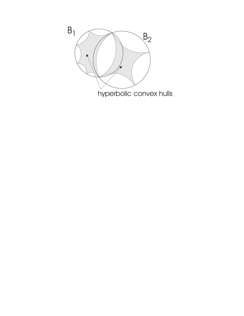
Figure 3. Maximal balls have disjoint hulls.

Lemma 3.3.

Suppose that $B_{1},B_{2}\in\mathfrak{B}^{\infty}$ with $B_{1}\neq B_{2}$. Then