Comparative Studies on Giant Magnetoresistance in Carbon Nanotubes and Graphene Nanoribbons with Ferromagnetic Contacts

Abstract

This contribution reports on comparative studies on giant magnetoresistance (GMR) in carbon nanotubes (CNTs) and graphene nanoribbons of similar aspect ratios (i.e perimeter/length and width/length ratios, for the former and the latter, respectively). The problem is solved at zero temperature in the ballistic transport regime, by means of the Green’s functions technique within the tight-binding model and with the so-called wide band approximation for electrodes. The GMR effect in graphene is comparable to that of CNTs, it depends strongly on the chirality and only slightly on the aspect ratio. It turns out that graphene, analogously to CNTs may be quite an interesting material for spintronic applications.

1 Introduction

Carbon-based structures evoke enormous interest in search for new materials for future nanoelectronics, expected to replace the conventional electronics soon. Along with carbon nanotubes [1], also graphene has recently given an additional impetus to this type of studies, after it was demonstrated that individual monolayers of graphite can be successfully fabricated and electrically contacted [2]. Although it has already been realized for several years that ferromagnetically contacted carbon nanotubes reveal quite a noticeable giant magnetoresistance (GMR) effect ([3] -[7]), in the case of grephene this problem still remains to be explored.

The paper is organized as follows: Sec. 2 presents the model and the adopted method of calculations, in Sec. 3 the results are presented and discussed. Finally, Sec. 4 summarizes the main conclusions.

2 Methodology

A single-band tight-binding model for non-interacting $\pi$-electrons is used both for CNTs and graphene (Gr):

$$H=\sum\limits_{i,\sigma}\varepsilon_{i}\left|i,\sigma\right\rangle\left\langle\sigma,i\right|+\sum\limits_{i,j,\sigma}t_{i,j}\left|i,\sigma\right\rangle\left\langle\sigma,j\right|,$$ (1)

In the following, the nearest neighbor hopping integral (typically equal to 2.7 - 3 eV) will be treated as the energy unit, t=1, whereas the on-site energies $\varepsilon$ depend on a gate voltage. The Hamiltonian [1] can be written in a tri-diagonal block form, each block (sub-matrix) is of rank equal to the number of atoms within the unit cell (N). For the armchair-CNT (ac-CNT) and zigzag-edge graphene (zz-Gr), as well as for the zigzag-CNT (zz-CNT) and armchair graphene (ac-Gr) structures discussed here $N=4n$, where $n$ is the component of the respective chiral vector $(n,n)$, $(n,0)$ for the ac-CNT and the zz-CNT. The unit cells are repeated periodically M times in the charge transport direction, resulting in 4nM atoms in the system. The present recursive method makes it possible, in principle, to perform recursive computations even for systems approaching realistic lengths of several hundred nm [8]. This time however relatively short systems are dealt with, because the systems of interest include also those with large transverse dimensions (exceeding the longitudinal ones).

As regards ferromagnetic leads (electrodes), the so called wide-band approximation has been used, i.e. the surface Green’s functions of the leads are treated as energy-independent, but spin-dependent (i.e. different for $\uparrow$- and $\downarrow$-spin electrons). The recursive method (see [9], [8]]) is described by the following set of equations:

$$g_{i,i}^{L}=(E-D_{i}-\Sigma_{i}^{L})^{-1},\;\;\;g_{i,i}^{R}=(E-D_{i}-\Sigma_{i}^{R})^{-1},$$ (2)

$$\Sigma_{i}^{L}=T_{i,i-1}g_{i-1,i-1}^{R}T_{i-1,i},\;\;\;\Sigma_{i}^{R}=T_{i,i+1}g_{i+1,i+1}^{R}T_{i+1,i},$$ (3)

$$G_{i}=(E-D_{i}-\Sigma_{i}^{L}-\Sigma_{i}^{R})^{-1}.$$ (4)

Eqs. (2) define Green’s functions for the i-th unit cell, the matrices D and T stand for the diagonal and off–diagonal sub-matrices, whereas the full Green’s function is given by Eq. 4. The carbon-based structure (either CNT or Gr) extends from i=1 up to i=M, whereas the left (L) and right (R) leads have indices $i<1$ and $i>M$, respectively. The simplest approximation one can think of, for the leads is the aforementioned wideband approximation. When applied to the present situation it corresponds to the following substitutions of the surface self-energies $\Sigma$’s by purely imaginary, energy-independent diagonal matrices:

$$\Sigma_{0}^{L}=-j\hat{1}\Delta_{L}/2,\;\;\;\Sigma_{M+1}^{R}=-j\hat{1}\Delta_{R}/2\;\;\;\;({\rm with}\;j=\sqrt{-1}).$$ (5)

The other quantities of the main interest here are transmission $\cal T$, conductance ($\cal G$) and giant magnetoresistance (GMR). In the ballistic transport regime and at zero temperature these quantities read:

$${\cal T}=Tr(\Gamma_{i}^{L}G_{i}\Gamma_{i}^{R}G_{i}^{\dagger}),\;\;\Gamma_{i}^{L,R}=j\left[\Sigma_{i}^{L,R}-\left(\Sigma_{i}^{L,R}\right)^{\dagger}\right],$$ (6)

$$GMR=100(1-{\cal G}_{\uparrow,\downarrow}/{\cal G}_{\uparrow,\uparrow}),\;\;\;{\cal G}=\frac{e^{2}}{h}{\cal T}(E_{F}),$$ (7)

where the arrows $\uparrow\uparrow$ and $\uparrow\downarrow$ denote prallel and anriparallel alignments of ferromagnetic electrodes. It is noteworthy that the transmission does not depend on the reference unit number $i$. The Fermi energy $E_{F}=0$ at zero gate voltage ($V_{G}$) and may be shifted in energy by $\alpha V_{G}$ for a finite gate voltage, where $\alpha$ is a conversion factor.

3 Results and discussion

The systems of interest here are CNTs and graphene ribbons of the same chirality, and similar aspect ratios defined as A=W/L, where L stands for the length and W for the width in the case of graphene, and the perimeter in the case of the CNT. An exemplary illustration of such systems is presented in Fig. 1.

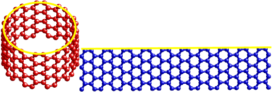
Fig. 1: Example of a CNT and a graphene sheet of similar aspect ratios. The leads are to be attached in the vertical direction both to the CNT and graphene.

In the case of ferromagnetic leads, the parameters $\Delta$ have been chosen as follows $\Delta_{L,R}^{\sigma}=\Delta_{0}(1\pm\sigma m)$, with $\Delta_{0}=0.6$, $m=1/3$. If the ferromagnetic leads are parallel aligned, the plus sign should be taken for both the sides (L and R), otherwise (antiparallel alignment) - the plus-sign applies to the L-lead and the minus-sign to the R-lead. The following two figures show how the GMR of CNTs and Gr sheets compare with each other for different aspect ratios (cf. (a) and (b)) and different chiralities (cf. Figs. 2, 3).

It is readily seen from these plots that the aspect ratio has some effect on the GMR. In particular, the long and narrow CNT show quasi-periodic behavior within the energy region below the onset to the higher sub-band, clearly revealing 2 and a half periods (see the first three narrow minima of the dashed line in Fig. 2a). The quasi-period is known to amount to $\hbar v_{F}/(2L)$. No distinct periodicity is seen in the case of graphene, where the longitudinal interference patterns are affected by the transverse modes and less pronounced Fabry-Perot patterns can be observe [10]. As shown in Fig. 2b the periodicity is lost even for the ac-CNT if the aspect ratio is high enough. It is so, since for $A>1$ the energy inter-level spacings ($\sim 1/L$) becomes comparable with the distance between the energy sub-bands ($\sim 1/W$).

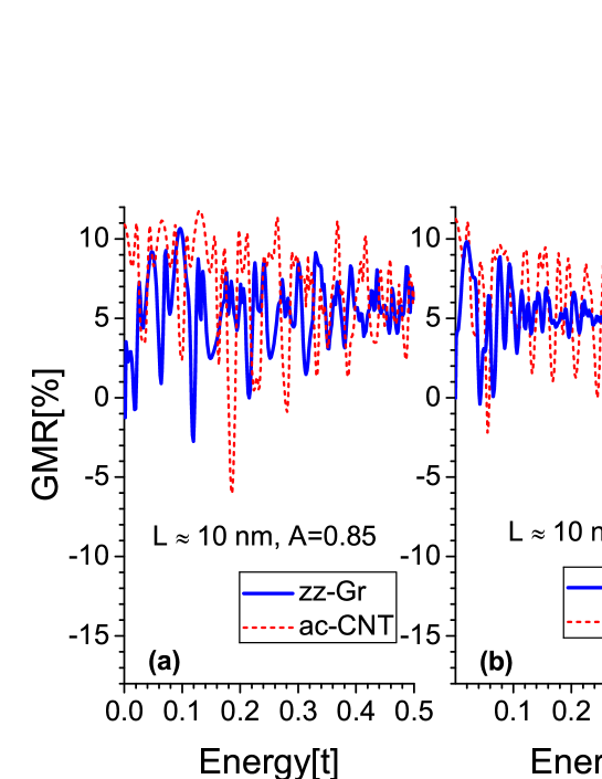
Fig. 2: GMR for ac-CNT (dashed line) and zz-graphene (solid line), and two different aspect ratios: less than 1 (a) and greater than 1 (b).

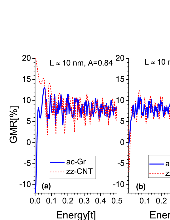
Fig. 3: As Fig. 2 but for different chiralities, i.e zz-CNT and ac-Gr.

As concerns the GMR, in the case of small $A$ negative values (inverse GMR) can be acquired, as already predicted theoretically for a more realistic model of electrodes [11] and observed experimentally [4]. This tendency may be explained basing on the Wigner-Breit formula for the on-resonance case and some anisotropy in CNT/electrode couplings. Interestingly for the present parametrization the average value of GMR changes roughly from 5% up to 10% for the zz-Gr, ac-CNT and ac-Gr, zz-CNT, respectively, i.e depends strongly on the chirality of the structure at hand, but only slightly on the aspect ratio. Nearby the charge neutrality point, $E_{F}=0$, the GMR behaves differently for the CNTs and graphene ribbons. This point is however very peculiar in many respects (massless fermions, minimum conductivity effect, non-negligible spin orbit coupling, etc.) and requires more sophisticated approach than the present one. It should be noticed in this context that here the spin-orbit (SO) coupling has been neglected. In the light of recent experiments [12] this is definitely justified in the case of graphene, but much less in the case of CNTs. Nevertheless, there is a consensus that SO coupling is not large enough to completely destroy the spin coherence (especially in short systems like those considered here).

4 Conclusion

Graphene ribbons show the GMR effect of comparable magnitude to CNTs with similar aspect ratios. The most important findings of the present studies are: (i) the mean value of GMR is bigger in ac-Gr than in zz-Gr, (ii) the fluctuations of GMR decrease with the increasing aspect ratio $A$, and (iii) for graphene the GMR fluctuations, as a function of energy (gate voltage), are smaller than those of its CNT counterpart.

Summarizing, both the carbon-based structures under consideration here seem to be quite promising for potential spintronic applications.

References

- [1] Saito R, Dresselhaus M S and Dresselhaus G, 1998 Physical Properties of Carbon Nanotubes, Imperial College Press.
- [2] K. S. Novoselov, A. K. Geim, S. V. Morozov, D. Jiang, M. I. Katsnelson, I. V. Grigorieva, S. V. Dubonos, and A. A. Firov, Nature, 438, 197 (2005).
- [3] K. Tsukagoshi, B. W. Alphenaar, and H. Ago, Nature 401, 572 (1999).
- [4] S. Sahoo, T. Kontos, J. Furer, C. Hoffmann, M. Graber, A. Cottet, and C. Schönenberger, Nature Physics 1, 99 (2005).
- [5] H. Mehrez, J. Taylor, H. Guo, J. Wang, and C. Roland, Phys. Rev. Lett. 84, 2682 (2000).
- [6] S. Krompiewski, Semicond. Sci. Technol. 21, S96 (2006).
- [7] S. Krompiewski, physica status solidi (b) 242 226 (2005).
- [8] S. Krompiewski, J. Martinek, and J. Barnaś, Phys. Rev. B 66, 073412 (2002).
- [9] R. Lake, G. Klimeck, R. C. Bowen, and D. Jovanovic, J. Appl. 81, 7845 (1997).
- [10] F. Miao, S. Wijeratne, Y. Zhang, U.C. Coskun, W. Bao, C.N. Lau, Science, 317, 1530 (2007).
- [11] S. Krompiewski, R. Gutierrez, and G. Cuniberti, Phys. Rev. B, 69, 155423 (2004).
- [12] F. Kuemmeth, S. Ilani, D. C. Ralph, and P. L. McEuen, Nature, 452, 448 (2008).