Fast Universal Algorithms for Robustness Analysis

Abstract

In this paper, we develop efficient randomized algorithms for estimating probabilistic robustness margin and constructing robustness degradation curve for uncertain dynamic systems. One remarkable feature of these algorithms is their universal applicability to robustness analysis problems with arbitrary robustness requirements and uncertainty bounding set. In contrast to existing probabilistic methods, our approach does not depend on the feasibility of computing deterministic robustness margin. We have developed efficient methods such as probabilistic comparison, probabilistic bisection and backward iteration to facilitate the computation. In particular, confidence interval for binomial random variables has been frequently used in the estimation of probabilistic robustness margin and in the accuracy evaluation of estimating robustness degradation function. Motivated by the importance of fast computing of binomial confidence interval in the context of probabilistic robustness analysis, we have derived an explicit formula for constructing the confidence interval of binomial parameter with guaranteed coverage probability. The formula overcomes the limitation of normal approximation which is asymptotic in nature and thus inevitably introduce unknown errors in applications. Moreover, the formula is extremely simple and very tight in comparison with classic Clopper-Pearson’s approach.

1 Introduction

In recent years, there have been growing interest on the development of probabilistic methods for robustness analysis and design problems aimed at overcoming the computational complexity and the issue of conservatism of deterministic worst case framework [21, 22, 19, 16, 24, 2, 5, 4, 23, 6, 7, 8, 9, 10, 26, 27, 20]. In the deterministic worst case framework, one is interested in computing the deterministic robustness margin which is defined as the maximal radius of uncertainty set such that the robustness requirement is guaranteed everywhere. However, it should be borne in mind that the uncertainty set may include worst cases which never happen in reality. Instead of seeking the worst case guarantee, it is sometimes “acceptable” that the robustness requirement is satisfied for most of the cases. It has been demonstrated that the proportion of systems guaranteeing the robustness requirement can be close to $1$ even if the radii of uncertainty set are much larger than the deterministic robustness margin. The idea of sacrificing extreme cases of uncertainty has become a new paradigm of robust control. In particular, the concept of probabilistic robustness margin has been recently established [2, 5, 24, 17, 4, 6, 23]. Moreover, to provide more insight for the robustness of the uncertain system, the concept of robustness degradation function has been developed by a number of researchers [2, 6]. For example, Barmish and Lagoa [5] have constructed a curve of robustness margin amplification versus risk in a probabilistic setting. In a similar spirit, Calafiore, Dabbene and Tempo [6, 7] have constructed a probability degradation function in the context of real and complex parametric uncertainty. Such a function describes quantitatively the relationship between the proportion of systems guaranteeing the robustness requirement and the radius of uncertainty set. Clearly, it can serve as a guide for control engineers in evaluating the robustness of a control system once a controller design is completed. It is important to note that the robustness degradation function and the probabilistic robustness margin can be estimated in a distribution free manner. This can be justified by the Truncation Theory established by Barmish, Lagoa and Tempo [2] and can also be illustrated by relaxing the deterministic worst-case paradigm.

Existing techniques for constructing the robustness degradation curve relies on the feasibility of computing the deterministic robustness margin. Obtaining the probabilistic robustness margin is possible only when the robustness degradation curve is constructed. However, the computation of deterministic robustness margin is possible only when the robustness requirement ${\bf P}$ is simple and the uncertainty bounding set is of some special structure. For example, ${\bf P}$ is stability requirement and uncertainty bounding sets are spectral normed balls. In that case, deterministic analysis methods such as $\mu$-theory can be applied to compute the deterministic robustness margin. The deterministic robustness margin is then taken as a starting point of uncertainty radius interval for which the robustness degradation curve is to be constructed. In general, the problem of computing the deterministic robustness margin is not tractable. Hence, to construct a robustness degradation curve of practical interest, the selection of uncertainty radius interval is itself a question. Clearly, the range of uncertainty radius for which robustness degradation curve is significantly below $1$ is not of practical interest since only a small risk can be tolerated in reality. From application point of view, it is only needed to construct robustness degradation curve for the range of uncertainty radius such that the curve is above an a priori specified level $1-\epsilon$ where risk parameter $\epsilon\in(0,1)$ is acceptably small.

In this work, we consider robustness analysis problems with arbitrary robustness requirement and uncertainty bounding set. We develop efficient randomized algorithms for estimating probabilistic robustness margin $\rho_{\epsilon}$ which is defined as the maximal uncertainty radius such that the probability of guaranteeing the robust requirements is at least $1-\epsilon$. We have also developed fast algorithms for constructing robustness degradation curve which is above a priori specified level $1-\epsilon$. In particular, we have developed efficient mechanisms such as probabilistic comparison, probabilistic bisection and backward iteration to reduce the computational complexity. Complexity of probabilistic comparison techniques are rigorously quantified.

In our algorithms, confidence interval for binomial random variables has been frequently used to improve the efficiency of estimating probabilistic robustness margin and in the accuracy evaluation of robustness degradation function. Obviously, fast construction of binomial confidence interval is important to the efficiency of the randomized algorithm. Therefore, we have derived an explicit formula for constructing the confidence interval of binomial parameter with guaranteed coverage probability [11]. The formula overcomes the limitation of normal approximation which is asymptotic in nature and thus inevitably introduce unknown errors in applications. Moreover, the formula is extremely simple and very tight in comparison with classic Clopper-Pearson’s approach.

The paper is organized as follows. Section 2 is the problem formulation. Section 2 discusses binomial confidence interval. Section 3 is devoted to probabilistic robustness margin. Section 4 presents algorithms for constructing robustness degradation curve. Illustrative examples are given in Section 5. Section 6 is the conclusion. Proofs are included in Appendix.

2 Problem Formulations

We adopt the assumption, from the classical robust control framework, that the uncertainty is deterministic and bounded. We formulate a general robustness analysis problem in a similar way as [10] as follows.

Let ${\bf P}$ denote a robustness requirement. The definition of ${\bf P}$ can be a fairly complicated combination of the following:

• Stability or ${\cal D}$-stability;

• $H_{\infty}$ norm of the closed loop transfer function;

• Time specifications such as overshoot, rise time, settling time and steady state error.

Let ${\cal B}(r)$ denote the set of uncertainties with size smaller than $r$. In applications, we are usually dealing with uncertainty sets such as the following:

• $l_{p}$ ball ${\cal B}^{p}(r):=\left\{\Delta\in{\bf R}^{n}:\;||\Delta||_{p}\leq r\right\}$ where $||.|_{p}$ denotes the $l_{p}$ norm and $p=1,2,\cdots,\infty$. In particular, ${\cal B}^{\infty}(r)$ denotes a box.

• Spectral norm ball ${\cal B}_{\sigma}(r):=\{\Delta\in{\bf\Delta}:\bar{\sigma}(\Delta)\leq r\}$ where $\bar{\sigma}(\Delta)$ denotes the largest singular value of $\Delta$. The class of allowable perturbations is

  $${\bf\Delta}:=\{{\rm blockdiag}[q_{1}I_{r_{1}},\cdots,q_{s}I_{r_{s}},\Delta_{1},\cdots,\Delta_{c}]\}$$ (1)

  where $q_{i}\in\mathbb{F},\;i=1,\cdots,s$ are scalar parameters with multiplicity $r_{1},\cdots,r_{s}$ and $\Delta_{i}\in\mathbb{F}^{n_{i}\times m_{i}},\;i=1,\cdots,c$ are possibly repeated full blocks. Here $\mathbb{F}$ is either the complex field ${\bf C}$ or the real field ${\bf R}$.

• Homogeneous star-shaped bounding set ${\cal B}_{H}(r):=\left\{r(\Delta-\Delta_{0})+\Delta_{0}:\Delta\in Q\right\}$ where $Q\subset{\bf R}^{n}$ and $\Delta_{0}\in Q$ (see [2] for a detailed illustration).

Throughout this paper, ${\cal B}(r)$ refers to any type of uncertainty set described above. Define a function $\ell(.)$ such that, for any $X$,

$$\ell(X):=\min\{r:X\in{\cal B}(r)\},$$

i.e., ${\cal B}(\ell(X))$ includes $X$ exactly in the boundary. By such definition,

$$\ell(X)=\min\left\{r:\frac{X-\Delta_{0}}{r}+\Delta_{0}\in Q\right\},$$

$$\ell(X)=\bar{\sigma}(X),$$

and

$$\ell(X)=||X||_{p}$$

in the context of homogeneous star-shaped bounding set, spectral norm ball and $l_{p}$ ball respectively.

To allow the robustness analysis be performed in a distribution-free manner, we introduce the notion of proportion as follows. For any $\Delta\in{\cal B}(r)$ there is an associated system $G(\Delta)$. Define proportion

$$\mathbb{P}(r):=\frac{{\rm vol}(\{\Delta\in{\cal B}(r):{\rm The\;associated\;system}\;G(\Delta)\;{\rm guarantees}\;{\bf P}\})}{{\rm vol}({\cal B}(r))}$$

with

$${\rm vol}(S):=\int_{q\in S}dq,$$

where the notion of $dq$ is illustrated as follows:

• (I): If $q=[x_{rs}]_{n\times m}$ is a real matrix in ${\bf R}^{n\times m}$, then $dq=\prod_{r=1}^{n}\prod_{s=1}^{m}dx_{rs}$.

• (II): If $q=[x_{rs}+jy_{rs}]_{n\times m}$ is a complex matrix in ${\bf C}^{n\times m}$, then $dq=\prod_{r=1}^{n}\prod_{s=1}^{m}(dx_{rs}dy_{rs})$.

• (III): If $q\in{\bf\Delta}$, i.e., $q$ possess a block structure defined by (1), then $dq=(\prod_{i=1}^{s}dq_{i})(\prod_{i=1}^{c}d\Delta_{i})$ where the notion of $dq_{i}$ and $d\Delta_{i}$ is defined by (I) and (II).

It follows that $\mathbb{P}(r)$ is a reasonable measure of the robustness of the system [6, 25]. In the worst case deterministic framework, we are only interested in knowing if ${\bf P}$ is guaranteed for every $\Delta$. However, one should bear in mind that the uncertainty set in our model may include worst cases which never happen in reality. Thus, it would be “acceptable” in many applications if the robustness requirement ${\bf P}$ is satisfied for most of the cases. Hence, due to the inaccuracy of the model, we should also obtain the value of $\mathbb{P}(r)$ for uncertainty radius $r$ which exceeds the deterministic robustness margin.

Clearly, $\mathbb{P}(r)$ is deterministic in nature. However, we can resort to a probabilistic approach to evaluate $\mathbb{P}(r)$. To see this, one needs to observe that a random variable with uniform distribution over ${\cal B}(r)$, denoted by ${\bf\Delta}^{u}$, guarantees that

$$\Pr\{{\bf\Delta}^{u}\in S\}=\frac{{\rm vol}(S\bigcap{\cal B}(r))}{{\rm vol}({\cal B}(r))}$$

for any $S$, and thus

$$\mathbb{P}(r)=\Pr\{{\rm The\;associated\;system}\;G({\bf\Delta}^{u})\;{\rm guarantees}\;{\bf P}\}.$$

Define a Bernoulli random variable $X$ such that $X$ takes value $1$ if the associated system $G({\bf\Delta}^{u})$ guarantees ${\bf P}$ and takes value $0$ otherwise. Then estimating $\mathbb{P}(r)$ is equivalent to estimating binomial parameter $\mathbb{P}_{X}:={\rm Pr}\{X=1\}=\mathbb{P}(r)$. It follows that a Monte Carlo method can be employed to estimate $\mathbb{P}(r)$ based on i.i.d. observations of $X$.

Obviously, the robustness problem will be completely solved if we can efficiently estimate $\mathbb{P}(r)$ for all $r\in(0,\infty)$. However, this is infeasible from computational perspective. In practice, only a small risk $\epsilon$ can be tolerated by a system. Therefore, what is really important to know is the value of $\mathbb{P}(r)$ over the range of uncertain radius $r$ for which $\mathbb{P}(r)$ is at least $1-\epsilon$ where $\epsilon\in(0,1)$ is referred as the risk parameter in this paper. When the deterministic robustness margin

$$\rho_{0}:=\sup\left\{r:\;G(\Delta)\;{\rm guarantees}\;{\bf P}\;{\rm for\;any}\;\Delta\in{\cal B}(r)\right\}$$

can be computed, we can construct the robustness degradation curve as follows: (I) Estimate proportion for a sequence of discrete values of uncertainty radius which is started from $r=\rho_{0}$ and gradually increased; (II) The construction process is continued until the proportion is below $1-\epsilon$. This is the conventional approach and it is feasible only when computing $\rho_{0}$ is tractable. Unfortunately, in general there exists no effective technique for computing the deterministic robustness margin $\rho_{0}$. In light of this situation, we establish a new approach which does not depend on the feasibility of computing the deterministic robustness margin. Our strategy is to firstly estimate the probabilistic robustness margin

$$\rho(\epsilon):=\sup\{r:\;\mathbb{P}(r)\geq 1-\epsilon\}$$

and consequently construct the robust degradation curve in a backward direction (in which $r$ is decreased) by choosing the estimate of $\rho(\epsilon)$ as the starting uncertainty radius.

To reduce computational burden, the estimation of probabilistic robustness margin relies on the frequent use of binomial confidence interval. The confidence interval is also served as a validation method for the accuracy of estimating robustness degradation function. Hence, it is desirable to quickly construct binomial confidence interval with guaranteed coverage probability.

3 Binomial Confidence Intervals

Clopper and Pearson [12] provided a rigorous approach for constructing binomial confidence interval. However, the computational complexity involved with this approach is very high. The standard technique is to use normal approximation which is not accurate for rare events. The coverage probability of the confidence interval derived from normal approximation can be significantly below the specified confidence level even for very large sample size. In the context of robustness analysis, we are dealing with rare events because the probability that the robustness requirement is violated is usually very small. We shall illustrate these standard methods as follows.

3.1 Clopper-Pearson Confidence Limits

Let the sample size $N$ and confidence parameter $\delta\in(0,1)$ be fixed. We refer an observation of $X$ with value 1 as a successful trial. Let $K$ denote the number of successful trials during the $N$ i.i.d. sampling experiments. Let $k$ be a realization of $K$. The classic Clopper-Pearson lower confidence limit $L_{N,k,\delta}$ and upper confidence limit $U_{N,k,\delta}$ are given respectively by

$$L_{N,k,\delta}:=\left\{\begin{array}[]{ll}0&{\rm if}\;k=0\\ \underline{p}&{\rm if}\;k>0\end{array}\right.\;\;\;{\rm and}\;\;\;U_{N,k,\delta}:=\left\{\begin{array}[]{ll}1&{\rm if}\;k=N\\ \overline{p}&{\rm if}\;k<N\end{array}\right.$$

where $\underline{p}\in(0,1)$ is the solution of the following equation

$$\sum_{j=0}^{k-1}{N\choose j}\underline{p}^{j}(1-\underline{p})^{N-j}=1-\frac{\delta}{2}$$ (2)

and $\overline{p}\in(0,1)$ is the solution of the following equation

$$\sum_{j=0}^{k}{N\choose j}\overline{p}^{j}(1-\overline{p})^{N-j}=\frac{\delta}{2}.$$ (3)

3.2 Normal Approximation

It is easy to see that the equations (2) and (3) are hard to solve and thus the confidence limits are difficult to determine using Clopper-Pearson’s approach. For large sample size, it is computationally intensive. To get around the difficulty, normal approximation has been widely used to develop simple approximate formulas (see, for example, [15] and the references therein). Let $\Phi(.)$ denote the normal distribution function and $Z_{\frac{\delta}{2}}$ denote the critical value such that $\Phi(Z_{\frac{\delta}{2}})=1-\frac{\delta}{2}$. It follows from the Central Limit Theorem that, for sufficiently large sample size $N$, the lower and upper confidence limits can be estimated respectively as $\widetilde{L}\approx\frac{k}{N}-Z_{\frac{\delta}{2}}\sqrt{\frac{\frac{k}{N}(1-\frac{k}{N})}{N}}$ and $\widetilde{U}\approx\frac{k}{N}+Z_{\frac{\delta}{2}}\sqrt{\frac{\frac{k}{N}(1-\frac{k}{N})}{N}}$.

The critical problem with the normal approximation is that it is of asymptotic nature. It is not clear how large the sample size is sufficient for the approximation error to be negligible. Such an asymptotic approach is not good enough for studying the robustness of control systems.

3.3 Explicit Formula

It is desirable to have a simple formula which is rigorous and very tight for the confidence interval construction. Recently, we have derived the following simple formula for constructing the confidence limits [11] (The proof is provided in Appendix for purpose of completeness).

Theorem 1

Let ${\cal L}(N,k,\delta)=\frac{k}{N}+\frac{3}{4}\;\frac{1-\frac{2k}{N}-\sqrt{1+4\theta\;k(1-\frac{k}{N})}}{1+\theta N}$ and ${\cal U}(N,k,\delta)=\frac{k}{N}+\frac{3}{4}\;\frac{1-\frac{2k}{N}+\sqrt{1+4\theta\;k(1-\frac{k}{N})}}{1+\theta N}$ with $\theta=\frac{9}{8\ln\frac{2}{\delta}}$. Then $\Pr\left\{{\cal L}(N,K,\delta)<\mathbb{P}_{X}<{\cal U}(N,K,\delta)\right\}>1-\delta$.

Figures 1 and 2 show the confidence limits derived by different methods (curve A and B represent respectively the upper and lower confidence limits computed by Theorem 1; curve C and D represent respectively the upper and lower confidence limits calculated by Clopper-Pearson’s method). It can be seen from these figures that our formula is very tight in comparison with the Clopper-Pearson’s approach. Obviously, there is no comparison on the computational complexity. Our formula is simple enough for hand calculation. Simplicity of the confidence interval is especially important in the context of our robustness analysis problem since the confidence limits are repeatedly used for a large number of simulations.

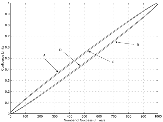
Figure 1: Confidence Interval ($N=1000,\;\delta=10^{-2}$)

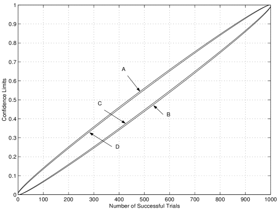
Figure 2: Confidence Interval ($N=1000,\;\delta=0.001$)

4 Estimating Probabilistic Robustness Margin

In this section, we shall develop efficient randomized algorithms for constructing an estimate for $\rho(\epsilon)$.

4.1 Separable Assumption

We assume that the robustness degradation curve of the system can be separated into two parts by a horizontal line with height $1-\epsilon$, i.e.,

$$\mathbb{P}(r)<1-\epsilon\;{\rm for\;all}\;r\geq\rho(\epsilon).$$

We refer such an assumption as the Separable Assumption. From an application point of view, this assumption is rather benign. Our extensive simulation experience indicated that, for small risk parameter $\epsilon$, most control systems guarantee the separable assumption. It should be noted that it is even much weaker than assuming that $\mathbb{P}(r)$ is non-decreasing (See illustrative Figure 3). Moreover, the non-increasing assumption is rather mild. This can be explained by a heuristic argument as follows. Let

$${\cal B}^{\bf P}(r):=\{\Delta\in{\cal B}(r):{\rm The\;associated\;system}\;G(\Delta)\;{\rm guarantees}\;{\bf P}\}.$$

Then

$$\mathbb{P}(r)=\frac{{\rm vol}({\cal B}^{\bf P}(r))}{{\rm vol}({\cal B}(r))}$$

and

$$\frac{d\mathbb{P}(r)}{dr}=\frac{1}{{\rm vol}({\cal B}(r))}\left[\frac{d\;{\rm vol}\{{\cal B}^{\bf P}(r)\}}{dr}-\mathbb{P}(r)\;\frac{d\;{\rm vol}\{{\cal B}(r)\}}{dr}\right].$$ (4)

Moreover, due to the constraint of robust requirement ${\bf P}$, it is true that ${\cal B}^{\bf P}(r+dr)\;\backslash\;{\cal B}^{\bf P}(r)$ is a subset of ${\cal B}(r+dr)\;\backslash\;{\cal B}(r)$ and it follows that ${\rm vol}\{{\cal B}(r)\}$ increases (as $r$ increases) faster than ${\rm vol}\{{\cal B}^{\bf P}(r)\}$, i.e., $\frac{d\;{\rm vol}\{{\cal B}^{\bf P}(r)\}}{dr}\leq\frac{d\;{\rm vol}\{{\cal B}(r)\}}{dr}$. Hence inequality $\frac{d\;{\rm vol}\{{\cal B}^{\bf P}(r)\}}{dr}\leq\mathbb{P}(r)\;\frac{d\;{\rm vol}\{{\cal B}(r)\}}{dr}$ is not hard to guarantee in the range of $r$ such that $\mathbb{P}(r)$ is close to $1$. It follows from equation (4) that $\frac{d\mathbb{P}(r)}{dr}\leq 0$ can be readily satisfied in the case of small risk parameter $\epsilon$.

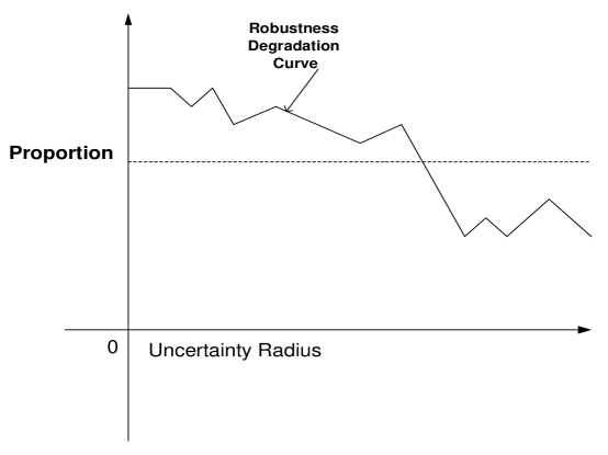
Figure 3: Illustration of Separable Assumption. The robustness degradation curve can be separated as the upper segment and lower segment by the dashed horizontal line with height $1-\epsilon$. In this example, the separable assumption is satisfied, while the non-increasing assumption is violated.

It is interesting to note that our randomized algorithms for estimating $\rho(\epsilon)$ presented in the sequel rely only on the following assumption:

$$\mathbb{P}(r)<1-\epsilon\;\;\forall r\in(\rho(\epsilon),2^{\kappa}]\bigcup\{2^{i}:\kappa<i\leq 0\}$$ (5)

where $\kappa=\lceil\log_{2}\rho(\epsilon)\rceil$. It can be seen that condition (5) is even weaker than the separable assumption.

When condition (5) is guaranteed, an interval which includes $\rho(\epsilon)$ can be readily found by starting from uncertainty radius $r=1$ and then successively doubling $r$ or cutting $r$ in half based on the comparison of $\mathbb{P}(r)$ with $1-\epsilon$. Moreover, bisection method can be employed to refine the estimate for $\rho(\epsilon)$. Of course, the success of such methods depends on the reliable and efficient comparison of $\mathbb{P}(r)$ with $1-\epsilon$ based on Monte Carlo method. In the following subsection, we illustrate a fast method of comparison.

4.2 Probabilistic Comparison

In general, $\mathbb{P}_{X}$ can only be estimated by a Monte Carlo method. The conventional method is to directly compare $\frac{K}{N}$ with $1-\epsilon$ where $K$ is the number of successful trials during $N$ i.i.d. sampling experiments. There are three problems with the conventional method. First, the comparison of $\frac{K}{N}$ with $1-\epsilon$ can be very misleading. Second, the sample size $N$ is required to be very large to obtain a reliable comparison. Third, we don’t know how reliable the comparison is. In this subsection, we present a new approach which allows for a reliable comparison with many fewer samples. The key idea is to compare binomial confidence limits with the fixed probability $1-\epsilon$ and hence reliable judgement can be made in advance.

Function name: Probabilistic-Comparison.

Input: Risk parameter $\epsilon$ and confidence parameter $\delta$.

Output: $d=$ Probabilistic-Comparison $(\delta,\epsilon)$.

Step $1$. Let $d\leftarrow 0$.

Step $2$. While $d=0$ do the following:

• Sample $X$.

• Update $N$ and $K$.

• Compute lower confidence limit $L$ and and upper confidence limit $U$ by Theorem 1.

• If $U<1-\epsilon$ then let $d\leftarrow-1$. If $L>1-\epsilon$ then let $d\leftarrow 1$.

The confidence parameter $\delta$ is used to control the reliability of the comparison. A typical value is $\delta=0.01$. The implication of output is as follows: $d=1$ indicates that $\mathbb{P}_{X}>1-\epsilon$ is true with high confidence; $d=-1$ indicates that $\mathbb{P}_{X}<1-\epsilon$ is true with high confidence.

Obviously, the sample size is random in nature. For $\epsilon=\delta=0.01$, we simulated the Probabilistic Comparison Algorithm identically and independently $100$ times for different values of $\mathbb{P}_{X}$. We observe that, for each value of $\mathbb{P}_{X}$, the Probabilistic Comparison Algorithm makes correct judgement among all $100$ simulations. Figure 4 shows the average sample size and the $95\%$-quantile of the sample size estimated from our simulation. It can be seen from the figure that, as long as $\mathbb{P}_{X}$ is not very close to $1-\epsilon$, the Probabilistic Comparison Algorithm can make a reliable comparison with a small sample size.

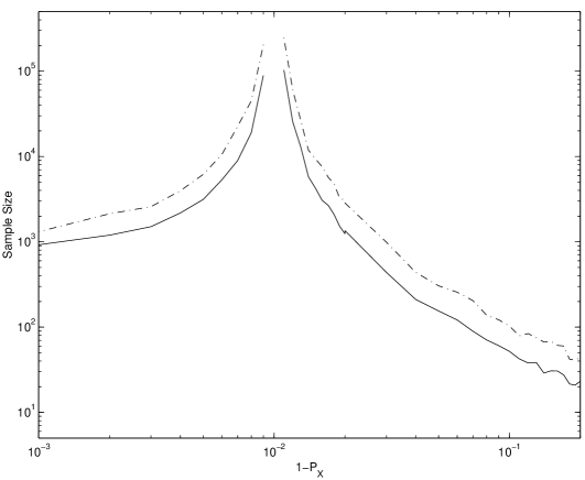
Figure 4: Complexity of Probabilistic Comparison. The horizontal axis represents $1-\mathbb{P}_{X}$. The vertical axis represents sample size. The solid line and the dash-dot line respectively show the average sample size and the $95\%$-quantile of the sample size.

4.3 Computing Initial Interval

Under the separable assumption, an interval $[a,b]$ which includes $\rho(\epsilon)$ can be quickly determined by the following algorithm.

Function name: Initial.

Input: Risk parameter $\epsilon$ and confidence parameter $\delta$.

Output: $[a,b]={\bf Initial}(\delta,\epsilon)$.

Step $1$. Let $r\leftarrow 1$. Apply Probabilistic-Comparison algorithm to compare $\mathbb{P}(1)$ with $1-\epsilon$. Let the outcome be $d_{1}$.

Step $2$. If $d_{1}=1$ then let $d\leftarrow d_{1}$ and do the following:

• While $d=1$ do the following:

  • Let $r\leftarrow 2r$. Apply Probabilistic-Comparison algorithm to compare $\mathbb{P}(r)$ with $1-\epsilon$. Let the outcome be $d$.

• Let $a\leftarrow\frac{r}{2}$ and $b\leftarrow r$.

Step $3$. If $d_{1}=-1$ then let $d\leftarrow d_{1}$ and do the following:

• While $d=-1$ do the following:

  • Let $r\leftarrow\frac{r}{2}$. Apply Probabilistic-Comparison algorithm to compare $\mathbb{P}(r)$ with $1-\epsilon$. Let the outcome be $d$.

• Let $a\leftarrow r$ and $b\leftarrow 2r$.

4.4 Probabilistic Bisection

Once an initial interval $[a,b]$ is obtained, an estimate $\widehat{R}$ for the probabilistic robustness margin $\rho(\epsilon)$ can be efficiently computed as follows.

Function name: Bisection.

Input: Risk parameter $\epsilon$, confidence parameter $\delta$, initial interval $[a,b]$, relative tolerance $\gamma$.

Output: $[\widehat{R}]={\bf Bisection}(\gamma,a,b,\delta,\epsilon)$.

Step $1$. Input $\gamma,\;a,\;b,\;\delta,\;\epsilon$.

Step $2$. While $b-a>\gamma a$ do the following:

• Let $r\leftarrow\frac{a+b}{2}$. Apply Probabilistic-Comparison algorithm to compare $\mathbb{P}(r)$ with $1-\epsilon$. Let the outcome be $d$.

• If $d=-1$ then let $b\leftarrow r$, else let $a\leftarrow r$.

Step $3$. Return $\widehat{R}=b$ (Note: this is actually a soft upper bound).

It should be noted that when applying bisection algorithm to refine the initial interval $[a,\;b]$, the execution of the algorithm may take very long time if $\mathbb{P}(r)\approx\epsilon$. However, such chance is almost $0$. This problem can be fixed by the following methods.

• We can limit the maximum number of simulations to a number $M$. When conducting simulation at radius $r$, simulation results can be saved for uncertainty radius $\frac{a+r}{2}$ where $a$ is the lower bound of the current interval with middle point $r$ (See the next section for the idea of sample reuse). After the number of simulations for uncertainty radius $r$ exceeds $M$, the simulation is switched for uncertainty radius $\frac{a+r}{2}$.

• In application, one might want to construct the robustness degradation curve in the backward direction by starting from an upper bound of $\rho(\epsilon)$. In that situation, we don’t need to compute a very tight interval for $\rho(\epsilon)$ and hence the chance of $\mathbb{P}(r)\approx\epsilon$ is even smaller.

5 Constructing Robustness Degradation Curve

We shall develop efficient randomized algorithms for constructing robustness degradation curve, which provide more insight for the robustness of the uncertain system than probabilistic robustness margin. First we recall the Sample Reuse algorithm [10] for constructing robustness degradation curve for a given range of uncertainty radius.

Sample Reuse Algorithm

Input: Sample size $N$, confidence parameter $\delta\in(0,1)$, uncertainty radius interval $[a,b]$, number of uncertainty radii $l$.

Output: Proportion estimate $\widehat{\mathbb{P}}_{i}$ and the related confidence interval for $r_{i}=b-\frac{(b-a)(i-1)}{l-1},\;\;i=1,2,\cdots,l$. In the following, $m_{i1}$ denotes the number of sampling experiments conducted at $r_{i}$ and $m_{i2}$ denotes the number of observations guaranteeing ${\bf P}$ during the $m_{i1}$ sampling experiments.

Step $1$ (Initialization). Let $M=[m_{ij}]_{l\times 2}$ be a zero matrix.

Step $2$ (Backward Iteration). For $i=1$ to $i=l$ do the following:

• Let $r\leftarrow r_{i}$.

• While $m_{i1}<N$ do the following:

  • Generate uniform sample $q$ from ${\cal B}(r)$. Evaluate the robustness requirement P for $q$.

  • Let $m_{s1}\leftarrow m_{s1}+1$ for any $s$ such that $r_{s}\geq\ell(q)$.

  • If robustness requirement P is satisfied for $q$ then let $m_{s2}\leftarrow m_{s2}+1$ for any $s$ such that $r_{s}\geq\ell(q)$.

• Let $\widehat{\mathbb{P}}_{i}\leftarrow\frac{m_{i2}}{N}$ and construct the confidence interval of confidence level $100(1-\delta)\%$ by Theorem $1$.

It should be noted that the idea of the Sample Reuse Algorithm is not simply a save of sample generation. It is actually a backward iterative mechanism. In the algorithm, the most important save of computation is usually the evaluation of the complex robustness requirements ${\bf P}$ (See [10] for details).

Now we introduce the global strategy for constructing robustness degradation curve. The idea is to successively apply the Sample Reuse Algorithm for a sequence of intervals of uncertainty radius. Each time the size of interval is reduced by half. The lower bound of the current interval is defined to be the upper bound of the next consecutive interval. The algorithm is terminated once the robustness requirement ${\bf P}$ is guaranteed for all $N$ samples of an uncertainty set of which the radius is taken as the lower bound of an interval of uncertainty radius. More precisely, the procedure is presented as follows.

Global Strategy

Input: Sample size $N$, risk parameter $\epsilon$ and confidence parameter $\delta\in(0,1)$.

Output: Proportion estimate $\widehat{\mathbb{P}}_{i}$ and the related confidence interval.

Step $1$. Compute an estimate $\widehat{R}$ for probabilistic robustness margin $\rho(\epsilon)$.

Step $2$. Let $STOP\leftarrow 0$. Let $a\leftarrow\frac{\widehat{R}}{2}$ and $b\leftarrow\widehat{R}$.

Step $3$ (Backward Iteration). While $STOP=0$ do the following:

• Apply Sample Reuse Algorithm to construct robustness degradation curve for uncertainty radius interval $[a,b]$.

• If the robustness property ${\bf P}$ is guaranteed for all $N$ samples of uncertainty set ${\cal B}(r)$ with radius $r=a$ then let $STOP\leftarrow 1$, otherwise let $b\leftarrow a$ and $a\leftarrow\frac{b}{2}$.

For given risk parameter $\epsilon$ and confidence parameter $\delta$, the sample size is chosen as

$$N>\frac{2(1-\epsilon+\frac{\alpha\epsilon}{3})(1-\frac{\alpha}{3})\ln\frac{2}{\delta}}{\alpha^{2}\epsilon}$$ (6)

with $\alpha\in(0,1)$. It follows from Massart’s inequality [18] that such a sample size ensures

$$\Pr\left\{\left|\mathbb{P}_{X}-\frac{K}{N}\right|<\alpha\epsilon\right\}>1-\delta$$

with $\mathbb{P}_{X}=1-\epsilon$ (See also Lemma 1 in Appendix). It should be noted that Massart’s inequality is less conservative than the Chernoff bounds in both multiplicative and additive forms.

We would like to remark that the algorithms we propose for estimating the probabilistic robustness margin and constructing robustness degradation curve are susceptible of further improvement. For example, the idea of sample reuse is not employed in computing the initial interval and in the probabilistic bisection algorithm. Moreover, in constructing the robustness degradation curve, the Sample Reuse Algorithm is independently applied for each interval of uncertainty radius. Actually, the simulation results can be saved for the successive intervals.

We would also like to note that, for a practitioner, computing the probabilistic robustness margin might be sufficient for understanding the system robustness. However, when more insight about the system robustness is expected, the techniques introduced in Section $5$ can be employed. Of course, the price is more computational effort.

6 Illustrative Examples

In this section we demonstrate through examples the power of our randomized algorithms in solving a wide variety of complicated robustness analysis problems which are not tractable in the classical deterministic framework.

We consider a system which has been studied in [14] by a deterministic approach. The system is as shown in Figure 5.

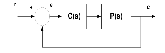
Figure 5: Uncertain System

The compensator is $C(s)=\frac{s+2}{s+10}$ and the plant is $P(s)=\frac{800(1+0.1\delta_{1})}{s(s+4+0.2\delta_{2})(s+6+0.3\delta_{3})}$ with parametric uncertainty $\Delta=[\delta_{1},\delta_{2},\delta_{3}]^{\rm T}$. The nominal system is stable. The closed-loop roots of the nominal system are:

$$z_{1}=-15.9178,\;\;z_{2}=-1.8309,\;\;z_{3}=-1.1256+7.3234i,\;\;z_{4}=-1.1256-7.3234i.$$

The peak value, rise time, settling time of step response of the nominal system, are respectively, $P_{peak}^{0}=1.47,\;\;t_{r}^{0}=0.185,\;\;t_{s}^{0}=3.175$.

We first consider the robust ${\cal D}$-stability of the system. The robustness requirement ${\bf P}$ is defined as ${\cal D}$-stability with the domain of poles defined as: Real part $<-1.5$, or fall within one of the two disks centered at $z_{3}$ and $z_{4}$ with radius $0.3$. The uncertainty set is defined as the polytope

$${\cal B}_{H}(r):=\left\{r\Delta+(1-r)\;\frac{\sum_{i=1}^{4}\Delta^{i}}{4}:\Delta\in{\rm conv}\{\Delta^{1},\Delta^{2},\Delta^{3},\Delta^{4}\}\right\}$$

where ‘conv’ denotes the convex hull of $\Delta^{i}=[\frac{1}{2}\sin(\frac{2i-1}{3}\pi),\;\frac{1}{2}\cos(\frac{2i-1}{3}\pi),\;-\frac{\sqrt{3}}{2}]^{\rm T}$ for $i=1,2,3$ and $\Delta^{4}=[0,\;0,\;1]^{\rm T}$.

Obviously, there exists no effective method for computing the deterministic robustness margin in the literature. However, our randomized algorithms can efficiently construct the robustness degradation curve. See Figure 6.

In this example, the risk parameter is a priori specified as $\epsilon=0.001$. The procedure for estimating the probabilistic robustness margin is explained as follows. Let $N$ denote the sample size which is random in nature. Let $K$ denote the number of successful trials among $N$ i.i.d. sampling experiments as defined in Section $2$ and Subsection $3.1$ (i.e., a successful trial is equivalent to an observation that the robustness requirement is guaranteed). Let confidence parameter $\delta=0.01$ and choose tolerance $\gamma=0.05$. Staring from $r=1$, after $N=7060$ simulations we obtain $K=7060$, the probabilistic comparison algorithm determined that $\mathbb{P}(1)>1-\epsilon$ since the lower confidence limit $L>1-\epsilon$. The simulation is thus switched to uncertainty radius $r=2$. After $N=65$ times of simulation, it is found that $K=61$. The probabilistic comparison algorithm detected that $\mathbb{P}(2)<1-\epsilon$ because the upper confidence limit $U<1-\epsilon$. So, initial interval $[1,2]$ is readily obtained. Now the probabilistic bisection algorithm is invoked. Staring with the middle point of the initial interval (i.e., $r=\frac{1+2}{2}=\frac{3}{2}$), after $N=613$ times of simulations, it is found that $K=607$, the probabilistic comparison algorithm concluded that $\mathbb{P}(\frac{3}{2})<1-\epsilon$ since the upper confidence limit $U<1-\epsilon$. Thus simulation is moved to $r=\frac{1+\frac{3}{2}}{2}=\frac{5}{4}$. It is found that $K=9330$ among $N=9331$ times of simulations. Hence, the probabilistic comparison algorithm determined that $\mathbb{P}(\frac{5}{4})>1-\epsilon$ since the lower confidence limit $L>1-\epsilon$. Now the simulation is performed at $r=\frac{\frac{5}{4}+\frac{3}{2}}{2}=\frac{11}{8}$. After $N=6653$ simulations, it is discovered that $K=6636$. The probabilistic comparison algorithm judged that $\mathbb{P}(\frac{11}{8})<1-\epsilon$ based on calculation that the upper confidence limit $U<1-\epsilon$. At this point the interval is $[\frac{5}{4},\frac{11}{8}]$ and the bisection is terminated since tolerance condition $b-a\leq\gamma a$ is satisfied. The evolution of intervals produced by the probabilistic bisection algorithm is as follows:

$$[1,2]\;\;\longrightarrow\;\;\left[1,\frac{3}{2}\right]\;\;\longrightarrow\;\;\left[\frac{5}{4},\frac{3}{2}\right]\;\;\longrightarrow\;\;\left[\frac{5}{4},\frac{11}{8}\right].$$

Now we have obtained an interval $[\frac{5}{4},\frac{11}{8}]$ which includes $\rho(0.001)$, so the Sample Reuse Algorithm can be employed to construct robustness degradation curve. In this example, the number of uncertainty radii is $l=100$ and the confidence parameter is chosen as $\delta=0.001$. A constant sample size is computed by formula (6) with $\alpha=0.5$ as

$$N=50,631.$$

The interval from which we start constructing robustness degradation curve is $[\frac{11}{16},\frac{11}{8}]$. It is determined that $K=N=50,632$ at uncertainty radius $r=\frac{11}{16}$. Therefore, the Sample Reuse Algorithm is invoked only once and the overall algorithm is terminated (If $K\neq N$ for $r=\frac{11}{16}$, then the next interval would be $[\frac{11}{32},\frac{11}{16}]$). Although $\mathbb{P}(r)$ is evaluated for $l=100$ uncertainty radii with the same sample size $N$, the total number of simulations is only $153,358<<Nl=100N$. To provide an evaluation of accuracy for all estimates of $\mathbb{P}(r)$, confidence limits are computed by Theorem $1$.

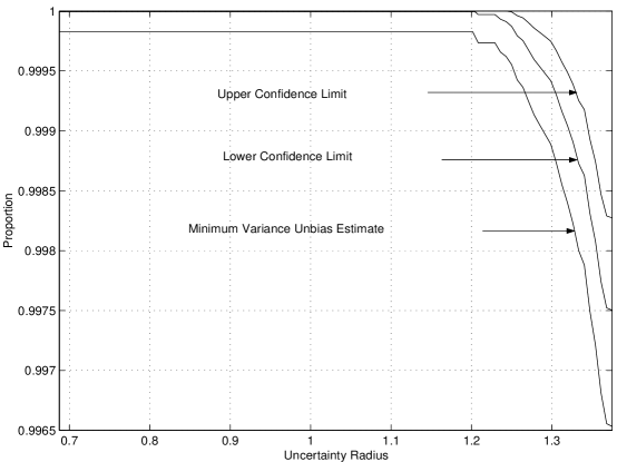
Figure 6: Robustness Degradation Curve

We now apply our algorithms to a robustness problem with time specifications. Specifically, the robustness requirement ${\bf P}$ is : Stability, and rise time $t_{r}<135\%\;t_{r}^{0}=0.25$, settling time $t_{s}<110\%\;t_{s}^{0}=3.5$, overshoot $P_{peak}<116\%\;P_{peak}^{0}=1.7$. The uncertainty set is ${\cal B}_{\infty}(r):=\{\Delta:\;||\Delta||_{\infty}\leq r\}$.

In this case, the risk parameter is a priori specified as $\epsilon=0.01$. It is well known that, for this type of problem, there exists no effective method for computing the deterministic robustness margin in the literature. However, our randomized algorithms can efficiently construct the robustness degradation curve. See Figure 7.

We choose $\gamma=0.25$ and $\delta=0.01$ for estimating $\rho(0.01)$. Starting from uncertainty radius $r=1$, the initial interval is easily found as $[\frac{1}{8},\frac{3}{16}]$ through the following interval evolution:

$$\left[\frac{1}{2},1\right]\;\;\longrightarrow\;\;\left[\frac{1}{4},\frac{1}{2}\right]\;\;\longrightarrow\;\;\left[\frac{1}{8},\frac{1}{4}\right].$$

The sequence of intervals generated by the probabilistic bisection algorithm is as follows:

$$\left[\frac{1}{8},\frac{1}{4}\right]\;\;\longrightarrow\;\;\left[\frac{1}{8},\frac{3}{16}\right]\;\;\longrightarrow\;\;\left[\frac{1}{8},\frac{5}{32}\right].$$

So, we obtained an estimate for the probabilistic robustness margin $\rho(0.01)$ as $\frac{5}{32}$. To construct robustness degradation curve, the number of uncertainty radii is chosen as $l=100$ and the confidence parameter is chosen as $\delta=0.01$. A constant sample size is computed by formula (6) with $\alpha=0.2$ as

$$N=24,495.$$

The interval from which we start constructing robustness degradation curve is $[\frac{5}{64},\frac{5}{32}]$. We found that this is also the last interval of uncertainty radius because it is determined that $K=N$ at uncertainty radius $r=\frac{5}{64}$.

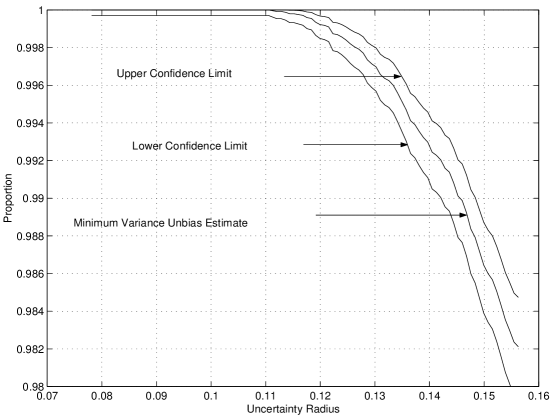
Figure 7: Robustness Degradation Curve

7 Conclusions

In this paper, we have established efficient techniques which applies to robustness analysis problems with arbitrary robustness requirements and uncertainty bounding set. The key mechanisms are probabilistic comparison, probabilistic bisection and backward iteration. Motivated by the crucial role of binomial confidence interval in reducing the computational complexity, we have derived an explicit formula for computing binomial confidence limits. This formula overcomes the computational issue and inaccuracy of standard methods.

Appendix A Proof of Theorem 1

To show Theorem 1, we need some preliminary results. The following Lemma 1 is due to Massart [18].

Lemma 1

${\Pr}\left\{\frac{K}{N}\geq\mathbb{P}_{X}+\epsilon\right\}\leq\exp\left(-\frac{N\epsilon^{2}}{2(\mathbb{P}_{X}+\frac{\epsilon}{3})\;(1-\mathbb{P}_{X}-\frac{\epsilon}{3})}\right)$ for all $\epsilon\in(0,1-\mathbb{P}_{X})$.

Of course, the above upper bound holds trivially for $\epsilon\geq 1-\mathbb{P}_{X}$. Thus, Lemma 1 is actually true for any $\epsilon>0$.

Lemma 2

${\Pr}\left\{\frac{K}{N}\leq\mathbb{P}_{X}-\epsilon\right\}\leq\exp\left(-\frac{N\epsilon^{2}}{2(\mathbb{P}_{X}-\frac{\epsilon}{3})\;(1-\mathbb{P}_{X}+\frac{\epsilon}{3})}\right)$ for all $\epsilon>0$.

Proof.

Define $Y=1-X$. Then $\mathbb{P}_{Y}=1-\mathbb{P}_{X}$. At the same time when we are conducting $N$ i.i.d. experiments for $X$, we are also conducting $N$ i.i.d. experiments for $Y$. Let the number of successful trials of the experiments for $Y$ be denoted as $K_{Y}$. Obviously, $K_{Y}=N-K$. Applying Lemma 1 to $Y$, we have ${\Pr}\left\{\frac{K_{Y}}{N}\geq\mathbb{P}_{Y}+\epsilon\right\}\leq\exp\left(-\frac{N\epsilon^{2}}{2(\mathbb{P}_{Y}+\frac{\epsilon}{3})\;(1-\mathbb{P}_{Y}-\frac{\epsilon}{3})}\right)$. It follows that ${\Pr}\left\{\frac{N-K}{N}\geq 1-\mathbb{P}_{X}+\epsilon\right\}\leq\exp\left(-\frac{N\epsilon^{2}}{2(1-\mathbb{P}_{X}+\frac{\epsilon}{3})\;[1-(1-\mathbb{P}_{X})-\frac{\epsilon}{3}]}\right)$. The proof is thus completed by observing that ${\Pr}\left\{\frac{N-K}{N}\geq 1-\mathbb{P}_{X}+\epsilon\right\}={\Pr}\left\{\frac{K}{N}\leq\mathbb{P}_{X}-\epsilon\right\}$. $\Box$

The following lemma can be found in [13].

Lemma 3

$\sum_{j=0}^{k}{N\choose j}x^{j}(1-x)^{N-j}$ decreases monotonically with respect to $x\in(0,1)$ for $k=0,1,\cdots,N$.

Lemma 4

$\sum_{j=0}^{k}{N\choose j}x^{j}(1-x)^{N-j}\leq\exp\left(-\frac{N(x-\frac{k}{N})^{2}}{2\;(\frac{2}{3}x+\frac{k}{3N})\;(1-\frac{2}{3}x-\frac{k}{3N})}\right)\;\;\forall x\in(\frac{k}{N},1)$ for $k=0,1,\cdots,N$.

Proof. Consider binomial random variable $X$ with parameter $\mathbb{P}_{X}>\frac{k}{N}$. Let $K$ be the number of successful trials during $N$ i.i.d. sampling experiments. Then $\sum_{j=0}^{k}{N\choose j}\mathbb{P}_{X}^{j}(1-\mathbb{P}_{X})^{N-j}={\rm Pr}\{K\leq k\}$. Note that ${\rm Pr}\{K\leq k\}={\rm Pr}\left\{\frac{K}{N}\leq\mathbb{P}_{X}-\left(\mathbb{P}_{X}-\frac{k}{N}\right)\right\}$. Applying Lemma 2 with $\epsilon=\mathbb{P}_{X}-\frac{k}{N}>0$, we have

$$\sum_{j=0}^{k}{N\choose j}\mathbb{P}_{X}^{j}(1-\mathbb{P}_{X})^{N-j} \leq \exp\left(-\frac{N(\mathbb{P}_{X}-\frac{k}{N})^{2}}{2(\mathbb{P}_{X}-\frac{\mathbb{P}_{X}-\frac{k}{N}}{3})\;(1-\mathbb{P}_{X}+\frac{\mathbb{P}_{X}-\frac{k}{N}}{3})}\right)$$

$$= \exp\left(-\frac{N(\mathbb{P}_{X}-\frac{k}{N})^{2}}{2\;(\frac{2}{3}\mathbb{P}_{X}+\frac{k}{3N})\;(1-\frac{2}{3}\mathbb{P}_{X}-\frac{k}{3N})}\right).$$

Since the argument holds for arbitrary binomial random variable $X$ with $\mathbb{P}_{X}>\frac{k}{N}$, thus the proof of the lemma is completed. $\;\;\;\;\square$

Lemma 5

$\sum_{j=0}^{k-1}{N\choose j}x^{j}(1-x)^{N-j}\geq 1-\exp\left(-\frac{N(x-\frac{k}{N})^{2}}{2\;(\frac{2}{3}x+\frac{k}{3N})\;(1-\frac{2}{3}x-\frac{k}{3N})}\right)\;\;\forall x\in(0,\frac{k}{N})$ for $k=1,\cdots,N$.

Proof. Consider binomial random variable $X$ with parameter $\mathbb{P}_{X}<\frac{k}{N}$. Let $K$ be the number of successful trials during $N$ i.i.d. sampling experiments. Then

$$\sum_{j=0}^{k-1}{N\choose j}\mathbb{P}_{X}^{j}(1-\mathbb{P}_{X})^{N-j}={\rm Pr}\{K<k\}={\rm Pr}\left\{\frac{K}{N}<\mathbb{P}_{X}+(\frac{k}{N}-\mathbb{P}_{X})\right\}.$$

Applying Lemma 1 with $\epsilon=\frac{k}{N}-\mathbb{P}_{X}>0$, we have that

$$\sum_{j=0}^{k-1}{N\choose j}\mathbb{P}_{X}^{j}(1-\mathbb{P}_{X})^{N-j} \geq 1-\exp\left(-\frac{N(\frac{k}{N}-\mathbb{P}_{X})^{2}}{2(\mathbb{P}_{X}+\frac{\frac{k}{N}-\mathbb{P}_{X}}{3})\;(1-\mathbb{P}_{X}-\frac{\frac{k}{N}-\mathbb{P}_{X}}{3})}\right)$$

$$= 1-\exp\left(-\frac{N(\mathbb{P}_{X}-\frac{k}{N})^{2}}{2\;(\frac{2}{3}\mathbb{P}_{X}+\frac{k}{3N})\;(1-\frac{2}{3}\mathbb{P}_{X}-\frac{k}{3N})}\right).$$

Since the argument holds for arbitrary binomial random variable $X$ with $\mathbb{P}_{X}<\frac{k}{N}$, thus the proof of the lemma is completed. $\;\;\;\;\square$

Lemma 6

Let $0\leq k\leq N$. Then $L_{N,k,\delta}<U_{N,k,\delta}$.

Proof. Obviously, the lemma is true for $k=0,N$. We consider the case that $1\leq k\leq N-1$. Define ${\cal S}(N,k,x):=\sum_{j=0}^{k}{N\choose j}x^{j}(1-x)^{N-j}$ for $x\in(0,1)$. Notice that ${\cal S}(N,k,\overline{p})={\cal S}(N,k-1,\overline{p})+{N\choose k}\overline{p}^{k}(1-\overline{p})^{N-k}=\frac{\delta}{2}$. Thus

$${\cal S}(N,k-1,\underline{p})-{\cal S}(N,k-1,\overline{p})=1-\frac{\delta}{2}-\left[\frac{\delta}{2}-{N\choose k}\overline{p}^{k}(1-\overline{p})^{N-k}\right].$$

Notice that $\delta\in(0,1)$ and that $\overline{p}\in(0,1)$, we have that

$${\cal S}(N,k-1,\underline{p})-{\cal S}(N,k-1,\overline{p})=1-\delta+{N\choose k}\overline{p}^{k}(1-\overline{p})^{N-k}>0.$$

By Lemma 3, ${\cal S}(N,k-1,x)$ decreases monotonically with respect to $x$, we have that $\underline{p}<\overline{p}$. $\;\;\;\;\square$

We are now in the position to prove Theorem 1. For national simplicity, let

$$p=U_{N,k,\delta},\;\;\;q={\cal U}(N,k,\delta).$$

It can be easily verified that $p\leq q$ for $k=0,\;N$. We need to show that $p\leq q$ for $0<k<N$. Straightforward computation shows that $q$ is the only root of equation

$$\exp\left(-\frac{N(x-\frac{k}{N})^{2}}{2\;(\frac{2}{3}x+\frac{k}{3N})\;(1-\frac{2}{3}x-\frac{k}{3N})}\right)=\frac{\delta}{2}$$

with respect to $x\in(\frac{k}{N},\infty)$. There are two cases: $q\geq 1$ and $q<1$. If $q\geq 1$ then $p\leq q$ is trivially true. We only need to consider the case that $\frac{k}{N}<q<1$. In this case, it follows from Lemma 4 that

$$\sum_{j=0}^{k}{N\choose j}{q}^{j}(1-q)^{N-j}\leq\exp\left(-\frac{N(q-\frac{k}{N})^{2}}{2\;(\frac{2}{3}q+\frac{k}{3N})\;(1-\frac{2}{3}q-\frac{k}{3N})}\right)=\frac{\delta}{2}.$$

Recall that

$$\sum_{j=0}^{k}{N\choose j}p^{j}(1-p)^{N-j}=\frac{\delta}{2},$$

we have

$$\sum_{j=0}^{k}{N\choose j}p^{j}(1-p)^{N-j}\geq\sum_{j=0}^{k}{N\choose j}{q}^{j}(1-q)^{N-j}.$$

Therefore, by Lemma 3, we have that $p\leq q$ for $0<k<N$. Thus, we have shown that $U_{N,k,\delta}\leq{\cal U}_{N,k,\delta}$ for all $k$.

Similarly, by Lemma 5 and Lemma 3 we can show that $L_{N,k,\delta}\geq{\cal L}(N,k,\delta)$. By Lemma 6, we have ${\cal L}(N,k,\delta)<L_{N,k,\delta}<U_{N,k,\delta}<{\cal U}(N,k,\delta)$. Finally, the proof of Theorem 1 is completed by invoking the probabilistic implication of the Clopper-Pearson confidence interval.

References

- [1] E. W. BAI, R. TEMPO, AND M. FU, “Worst-case properties of the uniform distribution and randomized algorithms for robustness analysis,” Mathematics of Control, Signals and Systems, vol. 11(1998), pp.183-196.
- [2] B. R. BARMISH, C. M. LAGOA, AND R. TEMPO, “Radially truncated uniform distributions for probabilistic robustness of control systems,” Proc. of American Control Conference, Albuquerque, New Mexico, June, 1997, pp. 853-857.
- [3] B. R. BARMISH, “A probabilistic result for a multilinearly parameterized norm,” Proc. of American Control Conference, Chicago, Illinois, June, 2000, pp. 3309-3310.
- [4] B. R. BARMISH AND B. T. POLYAK, “A new approach to open robustness problems based on probabilistic predication formulae,” IFAC’1996, San Francisco, Vol. H, pp. 1-6.
- [5] B. R. BARMISH AND C. M. LAGOA, “The uniform distribution: a rigorous justification for its use in robustness analysis,” Mathematics of Control, Signals and Systems, vol. 10 (1997), pp.203-222.
- [6] G. CALAFILORE, F. DABBENE, AND R. TEMPO, “Randomized algorithms for probabilistic robustness with real and complex structured uncertainty,” IEEE Transaction on Automatic Control, Vol. 45, No.12, December, 2000, pp. 2218-2235.
- [7] G. CALAFILORE, F. DABBENE, AND R. TEMPO, “Radial and uniform distributions in vector and matrix spaces for probabilistic robustness,” Topics in Control and Its Applications, Miller D. and Qiu L., Eds, Spring-Verlag, 1999, pp. 17-31.
- [8] X. CHEN AND K. ZHOU, “Order statistics and probabilistic robust control,” Systems and Control Letters, vol. 35(1998), pp. 175-182.
- [9] X. CHEN AND K. ZHOU, “Constrained robustness analysis and synthesis by randomized algorithms,” IEEE Transaction on Automatic Control, Vol. 45, No.6, June, 2000, pp. 1180-1186.
- [10] X. CHEN, K. ZHOU AND J. L. ARAVENA, “Fast construction of robustness degradation function”, Proceedings of Conference on Decision and Control, Las Vagas, Nevada, December 2002.
- [11] X. CHEN, K. ZHOU AND J. L. ARAVENA, “Explicit formula for constructing binomial confidence interval with guaranteed coverage probability,” Communications in Statistics — Theory and Methods, vol. 37, pp. 1173–1180, 2008.
- [12] C. J. CLOPPER and E. S. PEARSON, “The use of confidence or fiducial limits illustrated in the case of the binomial,” Biometrika, vol. 26, pp.404-413, 1934.
- [13] C. W. CLUNIES-ROSS, “Interval estimation for the parameter of a binomial distribution”, Biometrika, vol. 45, pp. 275-279, 1958.
- [14] R. R DE GASTON AND M. G. SAFONOV, “Exact calculation of the multiloop stability margin,” IEEE Trans. Autom. Control, vol. 33(1988), pp. 156-171.
- [15] A. HALD, Statistical Theory with Engineering Applications, pp. 697-700, John Wiley and Sons, 1952.
- [16] P. P. KHARGONEKAR AND A. TIKKU, “Randomized algorithms for robust control analysis and synthesis have polynomial complexity,” Proceedings of the 35th Conference on Decision and Control, Kobe, Japan, December 1996, pp. 3470-3475.
- [17] C. M. LAGOA, “Probabilistic enhancement of classic robustness margins: A class of none symmetric distributions ,” Proc. of American Control Conference, Chicago, Illinois, June, 2000, pp. 3802-3806.
- [18] P. MASSART, “The tight constant in the Dvoretzky-Kiefer-Wolfowitz inequality”, The Annals of Probability, pp. 1269-1283, Vol. 18, No. 3, 1990.
- [19] C. MARRISON AND R. F. STENGEL, “Robust control system design using random search and genetic algorithms,” IEEE Transaction on Automatic Control, Vol. 42, No.6, June, 1997, pp. 835-839.
- [20] S. R. ROSS AND B. R. BARMISH, “Distributionally Robust Gain Analysis for systems containing complexity,” Proceedings of the 40th Conference on Decision and Control, Orlando, Florida, December 2001, pp. 5020-5025.
- [21] L. R. RAY AND R. F. STENGEL, “A monte carlo approach to the analysis of control systems robustness,” Automatica, vol. 3(1993), pp. 229-236.
- [22] R. F. STENGEL AND L. R. RAY, “Stochastic robustness of linear time-invariant systems,” IEEE Transaction on Automatic Control, AC-36(1991), pp. 82-87.
- [23] B. T. POLYAK AND P. S. SHCHERABAKOV, “Random spherical uncertainty in estimation and robustness,” IEEE Trans. Autom. Control, vol. 45(2000), pp. 2145-2150.
- [24] R. TEMPO, E. W. BAI, AND F. DABBENE, “Probabilistic robustness analysis: explicit bounds for the minimum number of samples,” Systems and Control Letters, vol. 30 (1997), pp. 237-242.
- [25] R. TEMPO AND F. DABBENE, “Probabilistic robustness analysis and design of uncertain systems,” Progress in Systems and Control Theory, (ed. G. Picci) Birkhauser, March 1999, pp. 263-282.
- [26] M. VIDYASAGAR AND V. D. BLONDEL, “Probabilistic solutions to NP-hard matrix problems”, Automatica, vol. 37(2001), pp. 1597-1405.
- [27] M. VIDYASAGAR, “Randomized algorithms for robust controller synthesis using statistical learning theory”, Automatica, vol. 37(2001), pp. 1515-1528.