Sample Reuse Techniques of Randomized Algorithms for Control under Uncertainty

Abstract

Sample reuse techniques have significantly reduced the numerical complexity of probabilistic robustness analysis. Existing results show that for a nested collection of hyper-spheres the complexity of the problem of performing $N$ equivalent i.i.d. (identical and independent) experiments for each sphere is absolutely bounded, independent of the number of spheres and depending only on the initial and final radii.

In this chapter we elevate sample reuse to a new level of generality and establish that the numerical complexity of performing $N$ equivalent i.i.d. experiments for a chain of sets is absolutely bounded if the sets are nested. Each set does not even have to be connected, as long as the nested property holds. Thus, for example, the result permits the integration of deterministic and probabilistic analysis to eliminate regions from an uncertainty set and reduce even further the complexity of some problems. With a more general view, the result enables the analysis of complex decision problems mixing real-valued and discrete-valued random variables.

1 Introduction

The results presented in this chapter evolved from our previous work in probabilistic robustness analysis. For completeness we give a brief overview of the problem originally considered and show how it is embedded in our present, more general, formulation.

Probabilistic robust control methods have been proposed with the goal of overcoming the NP hard complexity and the conservatism associated with the deterministic worst-case framework of robust control (see, [1]–[26] and the references therein). At the heart of the probabilistic control paradigm is the idea of sacrificing the extreme instances of uncertainty. This is in sharp contrast to the deterministic robust control which approaches the issue of uncertainty with a “worst case” philosophy. Due to the obvious possibility of violation of robustness requirements associated with the probabilistic method, it has been the common contention that applying the probabilistic method for control design may be more dangerous than using the deterministic worst-case approach. Interestingly, it has been demonstrated (Chen, Aravena and Zhou, [8]) that it is not uncommon for a probabilistic controller (which guarantees only most instances of the uncertainty bounding set assumed in the design) to be significantly less risky than a deterministic worst-case controller. The reasons are the “uncertainty in modeling uncertainties” and the fact that the worst-case design cannot, in some instances, be “all encompassing.” Although this philosophy is proposed in the context of robust design, a direct consequence on robustness analysis is that it is not necessary to evaluate the system robustness in a deterministic worst-case framework. This is because a system certified to be robust in a deterministic worst-case framework is not necessarily less risky than a system with a probability that the robustness requirement is not always satisfied.

While the worst-case control theory uses the deterministic robustness margin to evaluate the system robustness, probabilistic control theory introduced the robustness function as a tool to measure the robustness properties of a control system subject to uncertainties. Such function is defined as

$$\mathbb{P}(r)=\mathrm{vol}(\{\text{$X\in\mathscr{B}_{r}\mid\mathbf{P}$ is guaranteed for $X$ }\})/\mathrm{vol}(\mathscr{B}_{r})$$

where $\mathrm{vol}(.)$ is the Lebesgue measure, $\mathbf{P}$ denotes the robustness requirement, and $\mathscr{B}_{r}$ denotes the uncertainty bounding set with radius $r$. This function describes quantitatively the relationship between the proportion of systems guaranteeing the robustness requirement and the radius of uncertainty set. Such a function has been proposed by a number of researchers. For example, Barmish and Lagoa [3] have constructed a curve of robustness margin amplification versus risk in a probabilistic setting.

The so-called robustness function can serve as a guide for control engineers in evaluating the robustness of a control system once a controller design is completed. In addition to overcome the issues of conservatism and NP complexity of the worst-case robustness analysis, the probabilistic robustness analysis based on the robustness function has the following advantages.

First, the robustness function can address problems which are intractable by deterministic worst-case methods. For many real world control problems, robust performance is more appropriately captured by multiple objectives such as stability, transient response (specified, for example, in terms of overshoot, rise time and settling time), disturbance rejection measured by $H_{\infty}$ or $H_{2}$ norm, etc. Thus, for a more insightful analysis of the robust performance of uncertain systems, the robustness requirement is usually multi-objective. The complexity of such robustness requirement can easily make the robustness problems intractable by the deterministic worst-case methods. For example, existing methods fail to solve robustness analysis problems when the robustness requirement is a combination of $H_{\infty}$ norm bound and stability. However, the robustness curve can still be constructed and provides sufficient insights on the robustness of the system.

Second, the probability that the robustness requirement is guaranteed can be inferred from the robustness function, while the deterministic margin has no relationship to such probability. Based on the assumption that the density function of uncertainty is radially symmetric and non-increasing with respect to the norm of uncertainty, it has been shown in [2] that the probability that $\mathbf{P}\;\mathrm{is\;guaranteed}$ is no less than $\inf_{\rho\in(0,r]}\mathbb{P}(\rho)$ when the uncertainty is contained in a bounding set with radius $r$. The underlying assumption is in agreement with conventional modeling and manufacturing practices that consider uncertainty as unstructured, with all directions equally likely, and make small perturbations more likely than large perturbations. It was discovered in [2] that the robustness function is not monotonically decreasing. Hence, the lower bound of the probability depends on $\mathbb{P}(\rho)$ for all $\rho\in(0,r]$. At the first glance, it may seem difficult or infeasible to estimate $\inf_{\rho\in(0,r]}\mathbb{P}(\rho)$ since the estimation of $\mathbb{P}(\rho)$ for every $\rho$ relies on the Monte Carlo simulation. For such probabilistic method to overcome the NP hard of worst-case methods, it is necessary to show that the complexity for estimating $\inf_{\rho\in(0,r]}\mathbb{P}(\rho)$ for a given $r$ is polynomial in terms of computer running time and memory space. Recently, sample reuse techniques have been developed in [7, 9, 10] and it is demonstrated that the complexity in terms of space and time is surprisingly low and is linear in the uncertainty dimension and the logarithm of the relative width of the range of uncertainty radius.

Third, using the robustness function for the evaluation of the system robustness allows the designer to make more accurate statements than using just the robustness margins. Here, by robustness margins, we mean both the deterministic robustness margin and its risk-adjusted version – the probabilistic robustness margin, defined as $\rho_{\varepsilon}=\sup\{r\mid\mathbb{P}(r)\geq 1-\varepsilon\}$. For virtually all practical systems, the deterministic robustness margin can be viewed as a special case of the probabilistic robustness margin $\rho_{\varepsilon}$ with $\varepsilon=0$. This property should not be confused with the numerical accuracy in evaluating margins nor with the issue of conservatism. The fundamental reason is the lack of information that can be available from the robustness margins. It has been demonstrated in [9, 10] that both the deterministic and probabilistic robustness margins have inherent limitations. In other words, using $\rho_{\varepsilon}$ as a measure of robustness can be misleading. Figure 1 shows the conceptual robustness functions for two controllers. From the figure it is apparent that the robustness margin with $\varepsilon\in[0,0.005]$, $\rho_{\varepsilon}^{A}$, for controller $A$ is much larger than the corresponding value, $\rho_{\varepsilon}^{B}$, for controller $B$. Then, based on the comparison of $\rho_{\varepsilon}$, control systems $A$ is certainly more robust and should be recommended for safety purposes. However, if the coverage probability of the uncertainty set $\mathscr{B}_{\rho_{\varepsilon}^{A}}$ is low and the robustness curve (i.e, the graphical representation of the robustness function) of control system $A$ rolls off rapidly beyond $\rho_{\varepsilon}^{A}$, then the robustness of system $A$ may be poor. On the other hand, if the robustness curve of control system $B$ maintains a high level for a wide range of uncertainty radius, then control system $B$ may be actually more robust than system $A$.

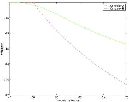
Figure 1: Comparison of Controller Alternatives

In general, the evaluation of the robustness function requires extensive Monte Carlo simulations. In applications, many iterations of robust design and analysis may be needed in the development of a satisfactory control system, it is therefore crucial to improve the efficiency of estimating the robustness function. Complexity has been reduced by considering models for the uncertainties that depend on a single “uncertainty radius.” In this case, the formal evaluation of the robustness function requires $N$, i.i.d. uncertain parameter selections for each of a sequence $r_{1}<r_{2}<\dots<r_{m}$ of uncertainty radii, which is still a daunting task. The sample reuse principle allows carrying the evaluation to any degree of accuracy and with absolute bounds in complexity (see, [7, 9, 10]).

The use of uncertainty bounding sets with a given radius can still be viewed as a limitation since one may have to include situations that never arise in practice. This is the limitation addressed in this work. Moreover, we cast to result as a general problem in decision-making under uncertainties. We show that the sample reuse principle can be applied with equal effectiveness in a much more general scenario. We shall be concerned with an arbitrary sequence of nested sets $\mathscr{B}_{1}\subset\mathscr{B}_{2}\subset\cdots\subset\mathscr{B}_{m}$ where we need to perform $N$ experiments for elements uniformly and independently drawn from each set. For each element it is necessary to verify if a certain statement $\mathbf{P}$ is true or not.

The idea of the sample reuse principle is to start experiments from the largest set and if it also belongs to smaller subset the experimental result is saved for later use in the smaller set. The experimental result that can be saved includes not only the samples from the sets but also the outcome of the evaluation of the statement $\mathbf{P}$. We note that this formulation enables the efficient use of Monte Carlo simulations for the evaluation of multi-dimensional distributions and the combination of continuous and discrete variables.

2 Absolute Bound of Complexity

Consider a sequence of nested sets $\mathscr{B}_{1}\subset\mathscr{B}_{2}\subset\cdots\subset\mathscr{B}_{m}$. If one needs to perform $N$ experiments from each set, a conventional approach would require a total of $Nm$ experiments. However, due to sample reuse, the actual number of experiments for set $\mathscr{B}_{i}$ is a random number ${\bf n}_{i}$, which is usually less than $N$. Our main result, which depends only on the nested property, shows that this strategy saves a significant amount of experimental or computational effort.

Theorem 1

Let $V_{\mathrm{min}}$ and $V_{\mathrm{max}}$ be constants such that $0<V_{\mathrm{min}}\leq V_{\mathrm{max}}<\infty$. For an arbitrary sequence of nested sets $\mathscr{B}_{i},\;i=1,\cdots,m$ such that $\mathscr{B}_{1}\subset\mathscr{B}_{2}\subset\cdots\subset\mathscr{B}_{m}$ and $V_{\mathrm{min}}\leq\mathrm{vol}(\mathscr{B}_{1})\leq\mathrm{vol}(\mathscr{B}_{m})\leq V_{\mathrm{max}}$, the expected total number of experiments, $\boldsymbol{n}$, to obtain $N$ experiments for each set is absolutely bounded, independent of the number, $m$, of sets in the chain and given by

$$\boxed{\mathbb{E}\left[\boldsymbol{n}\right]<\left(1+\ln\frac{V_{\mathrm{max}}}{V_{\mathrm{min}}}\right)N}$$

where $\mathbb{E}[.]$ denotes the expectation of a random variable.

Remark 1

The fact that the result is independent of the number of sets in the nested chain may appear surprising but it is a direct consequence of the power of the sample reuse principle. Loosely speaking, the more sets are there in the chain, the more chances that an experiment can be reused. In fact this characteristic makes the result especially powerful when the demands for accuracy, indicated by a large number of sets, is high.

As a special case of Theorem 1, we have the following result, reported by Chen, Zhou, Aravena [9, 10] and presented here now as a corollary to our main result.

Corollary 1

Let $r_{\mathrm{min}}$ and $r_{\mathrm{max}}$ be constants such that $0<r_{\mathrm{min}}\leq r_{\mathrm{max}}<\infty$. Let $B_{r}$ denote the uncertainty bounding sets with radius $r$. Suppose that $\mathrm{vol}(B_{r})=r^{d}\mathrm{vol}(B_{1})$ for any radius $r$. Then, for any sequence of radius $r_{1}<r_{2}<\cdots<r_{m}$ such that $r_{\mathrm{min}}\leq r_{1}<r_{m}\leq r_{\mathrm{max}}$,

$$\mathbb{E}\left[\boldsymbol{n}\right]<\left(1+d\ln\frac{r_{\mathrm{max}}}{r_{\mathrm{min}}}\right)N.$$

2.1 Observations about the result

In the result presented here, the only requirement for the uncertainty sets is that they must be nested. This is in sharp contrast to the existing model of uncertainty wherein we define an uncertainty “radius” and larger uncertainty sets are simply amplified versions of the smaller sets, defining a chain of sets of essentially the same shape. Such limitation is completely eliminated now.

Another significant feature of the new result is that the uncertainty sets can have “holes” in them; i.e., one can easily eliminate situations, or values, that cannot physically take place. In a later section we examine this option in more detail and show the advantage provided by the general result.

In fact, as long as the sets are nested, the sets don’t even have to be connected. This permits modeling of situations that were not feasible, for example, combination of discrete and continuous-valued random variables.

Finally, the power of the result lies in the efficient use of experiments. The property that is being tested is not germane to the result. In this sense, we have provided a tool for decision making in complex environments.

3 Proof of Main Theorem

This section provides a formal proof of our main result. First we establish some preliminary results that will be needed in the proof.

Lemma 1

For $i=2,\ldots,m$,

$$\mathbb{E}\left[{\bf n}_{i-1}\right]=N-\sum_{j=i}^{m}\left(\frac{v_{i-1}}{v_{j}}\right)\;\mathbb{E}\left[{\bf n}_{j}\right]$$

where $v_{j}=\mathrm{vol}(\mathscr{B}_{j}),\;j=1,\cdots,m$.

Proof.

Let $m\geq j\geq i\geq 2$. Let $q^{1},q^{2},\ldots,q^{{\bf n}_{j}}$ be the samples generated from $\mathscr{B}_{j}$. For $\ell=1,\ldots,{\bf n}_{j}$, define random variable $X_{j,i-1}^{\ell}$ such that

$$X_{j,i-1}^{\ell}\stackrel{{\scriptstyle\mathrm{def}}}{{=}}\left\{\begin{array}[]{ll}1&\mathrm{if}\;q^{\ell}\;\mathrm{fall\;in}\;\mathscr{B}_{i-1},\\ 0&\mathrm{otherwise.}\end{array}\right.$$

Based on the principle of sample reuse, we have

$${\bf n}_{m}=N,\qquad{\bf n}_{j}=N-\sum_{k=j+1}^{m}\sum_{\ell=1}^{{\bf n}_{k}}X_{k,j}^{\ell},\qquad j=1,\cdots,m-1,$$

which implies that the value of ${\bf n}_{j}$ depends only on the samples generated from sets $\mathscr{B}_{k},\;j+1\leq k\leq m$. Hence, event $\{{\bf n}_{j}=n\}$ is independent of event $\{X_{j,i-1}^{\ell}=1\}$. It follows that

$$\Pr\left\{X_{j,i-1}^{\ell}=1,\;{\bf n}_{j}=n\right\}=\Pr\left\{X_{j,i-1}^{\ell}=1\right\}\Pr\left\{{\bf n}_{j}=n\right\}$$

where $\Pr\{.\}$ denotes the probability of an event. Recall that $q^{\ell}$ is a random variable with uniform distribution over $\mathscr{B}_{j}$, we have

$$\Pr\left\{X_{j,i-1}^{\ell}=1\right\}=\frac{v_{i-1}}{v_{j}},\qquad\ell=1,\cdots,N.$$

By the principle of sample reuse,

$$N={\bf n}_{i-1}+\sum_{j=i}^{m}\sum_{\ell=1}^{{\bf n}_{j}}X_{j,i-1}^{\ell}.$$

Thus for $i=2,\ldots,m$,

$$\mathbb{E}\left[{\bf n}_{i-1}\right] = N-\sum_{j=i}^{m}\mathbb{E}\left[\sum_{\ell=1}^{{\bf n}_{j}}X_{j,i-1}^{\ell}\right]$$

$$= N-\sum_{j=i}^{m}\sum_{n=1}^{N}\sum_{\ell=1}^{n}\Pr\left\{X_{j,i-1}^{\ell}=1,\;{\bf n}_{j}=n\right\}$$

$$= N-\sum_{j=i}^{m}\sum_{n=1}^{N}\sum_{\ell=1}^{n}\Pr\left\{X_{j,i-1}^{\ell}=1\right\}\Pr\{{\bf n}_{j}=n\}$$

$$= N-\sum_{j=i}^{m}\sum_{n=1}^{N}n\left(\frac{v_{i-1}}{v_{j}}\right)\Pr\{{\bf n}_{j}=n\}$$

$$= N-\sum_{j=i}^{m}\left(\frac{v_{i-1}}{v_{j}}\right)\sum_{n=1}^{N}n\Pr\{{\bf n}_{j}=n\}$$

$$= N-\sum_{j=i}^{m}\left(\frac{v_{i-1}}{v_{j}}\right)\;\mathbb{E}\left[{\bf n}_{j}\right].\qquad$$

$\Box$

This result gives the expected number of experiments for a set, $\mathscr{B}_{i-1}$, in terms of the expected values for all the sets that contain it. The recursion can be solved as follows: Since all the experiments must belong to the set $\mathscr{B}_{m}$ we have $\mathbb{E}[{\bf n}_{m}]=N$, now for $i<m$ we can write

$$\mathbb{E}\left[{\bf n}_{i}\right]=N-\sum_{j=i+1}^{m}\left(\frac{v_{i}}{v_{j}}\right)\;\mathbb{E}\left[{\bf n}_{j}\right]\quad\Longrightarrow\quad\sum_{j=i+1}^{m}\left(\frac{v_{i}}{v_{j}}\right)\;\mathbb{E}\left[{\bf n}_{j}\right]=N-\mathbb{E}\left[{\bf n}_{i}\right]$$

and

$$\mathbb{E}\left[{\bf n}_{i-1}\right] = N-\sum_{j=i}^{m}\left(\frac{v_{i-1}}{v_{j}}\right)\;\mathbb{E}\left[{\bf n}_{j}\right]$$

$$= N-\left(\frac{v_{i-1}}{v_{i}}\right)\mathbb{E}\left[{\bf n}_{i}\right]-\sum_{j=i+1}^{m}\left(\frac{v_{i-1}}{v_{j}}\right)\mathbb{E}\left[{\bf n}_{j}\right]$$

$$= N-\left(\frac{v_{i-1}}{v_{i}}\right)\mathbb{E}\left[{\bf n}_{i}\right]-\left(\frac{v_{i-1}}{v_{i}}\right)\sum_{j=i+1}^{m}\left(\frac{v_{i}}{v_{j}}\right)\mathbb{E}\left[{\bf n}_{j}\right].$$

Therefore,

$$\mathbb{E}\left[{\bf n}_{i-1}\right] = N-\left(\frac{v_{i-1}}{v_{i}}\right)\mathbb{E}\left[{\bf n}_{i}\right]-\left(\frac{v_{i-1}}{v_{i}}\right)\left[N-\mathbb{E}\left[{\bf n}_{i}\right]\right]$$

$$= N-\left(\frac{v_{i-1}}{v_{i}}\right)N.$$

Thus we have established

Lemma 2

Under the sample reuse principle, for an arbitrary sequence of nested sets $\mathscr{B}_{i},\;i=1,\cdots,m$ such that $\mathscr{B}_{1}\subset\mathscr{B}_{2}\subset\cdots\subset\mathscr{B}_{m}$ and $0<\mathrm{vol}(\mathscr{B}_{1})\leq\mathrm{vol}(\mathscr{B}_{m})<\infty$, the expected total number of experiments, $\mathbb{E}\left[{\bf n}_{i}\right]$, to obtain $N$ experiments for the set $\mathscr{B}_{i}$ is

$$\mathbb{E}({\bf n}_{i})=N-\frac{v_{i}}{v_{i+1}}N;\quad i=1,2,\dots,m-1.$$

Remark 2

We note that if we use the convention $v_{m+1}=\infty$ then the previous expression can be made valid for $i=m$.

Once more one can see the power of the sample reuse principle. If any two sets in the chain are “very similar,” then most of the experiments for the larger set can be reused.

Now we establish a basic inequality that will be used to prove the main result.

Lemma 3

For any $x>1$,

$$\frac{1}{x}+\ln x>1.$$

Proof. Let

$$f(x)=\frac{1}{x}+\ln x.$$

Then $f(1)=1$ and

$$\frac{d\;f(x)}{dx}=\frac{x-1}{x^{2}}>0,\qquad\forall x>1.$$

It follows that $f(x)>1,\;\forall x>1$. $\Box$

Using the previous result now we can prove

Lemma 4

For an arbitrary sequence of numbers $0<r_{1}<r_{2}<\cdots<r_{m}$,

$$m-\sum_{i=1}^{m-1}\frac{r_{i}}{r_{i+1}}<1+\ln\left(\frac{r_{m}}{r_{1}}\right).$$

Proof.

Observing that

$$\frac{r_{m}}{r_{1}}=\prod_{i=1}^{m-1}\frac{r_{i+1}}{r_{i}},$$

we have

$$\ln\left(\frac{r_{m}}{r_{1}}\right)=\sum_{i=1}^{m-1}\ln\left(\frac{r_{i+1}}{r_{i}}\right).$$

Therefore,

$$\sum_{i=1}^{m-1}\frac{r_{i}}{r_{i+1}}+\ln\left(\frac{r_{m}}{r_{1}}\right) = \sum_{i=1}^{m-1}\left[\frac{1}{\frac{r_{i+1}}{r_{i}}}+\ln\left(\frac{r_{i+1}}{r_{i}}\right)\right].$$

Since $\frac{r_{i+1}}{r_{i}}>1,\;i=1,\cdots,m-1$, it follows from Lemma 3 that

$$\frac{1}{\frac{r_{i+1}}{r_{i}}}+\ln\left(\frac{r_{i+1}}{r_{i}}\right)>1,\qquad i=1,\cdots,m-1.$$

Hence,

$$\sum_{i=1}^{m-1}\frac{r_{i}}{r_{i+1}}+\ln\left(\frac{r_{m}}{r_{1}}\right)>m-1.$$

The lemma is thus proved.

$\Box$

Now we are in the position to prove Theorem 1. By Lemma 2, we have

$$\mathbb{E}[\boldsymbol{n}] = \mathbb{E}\left[\sum_{i=1}^{m}{\bf n}_{i}\right]$$

$$= N+\sum_{i=1}^{m-1}\left[N-N\left(\frac{v_{i}}{v_{i+1}}\right)\right]$$

$$= Nm-N\;\sum_{i=1}^{m-1}\frac{v_{i}}{v_{i+1}}.$$

Therefore, by Lemma 4,

$$\mathbb{E}\left[\frac{\boldsymbol{n}}{N}\right]=m-\sum_{i=1}^{m-1}\frac{v_{i}}{v_{i+1}}<1+\ln\left(\frac{v_{m}}{v_{1}}\right)\leq\left(1+\ln\frac{V_{\mathrm{max}}}{V_{\mathrm{min}}}\right)$$

and thus the proof of Theorem 1 is completed.

4 Combination with Deterministic Methods

In this section we demonstrate the flexibility allowed by the general nested conditions by examining a situation that could not be properly handled with existing tools. Especially, we consider uncertainty sets where, for example by deterministic analysis, one can establish subsets that are not feasible; i.e., the uncertainty set has “holes” in it.

There exist rich results for computing the exact or conservative bounds of the robustness margins, e.g., structure singular value $\mu$ theory or Kharitonov type methods. Let $S_{r}$ be a hyper-sphere with radius $r$. Suppose the robustness requirement is satisfied for the nominal system. By the deterministic approach, in some situations, it may be possible to determine $r_{0}$ such that the robustness requirement is satisfied for $S_{r_{0}}$. Then, to estimate

$$\mathbb{P}(r)=\frac{\mathrm{vol}(\{q\in S_{r}\mid\mathbf{P}\;\text{is guaranteed for }\;q\})}{\mathrm{vol}(S_{r})}$$

for $r_{1}<r_{2}<\cdots<r_{m}$ with $r_{1}>r_{0}$, we can apply the sample reuse techniques over a nested chain of “donut” sets $D_{1}\subset D_{2}\subset\cdots\subset D_{m}$ with

$$D_{i}=S_{r_{i}}\setminus S_{r_{0}},\quad i=1,\cdots,m$$

where “$\setminus$” denotes the operation of set minus. Instead of directly estimate $\mathbb{P}(r_{i})$, we can estimate

$$\wp_{i}=\frac{\mathrm{vol}(\{q\in D_{i}\mid\mathbf{P}\;\text{is guaranteed for }\;q\})}{\mathrm{vol}(D_{i})}$$

and obtain

$$\mathbb{P}(r_{i})=\frac{\wp_{i}\;\mathrm{vol}(D_{i})+\mathrm{vol}(S_{r_{0}})}{\mathrm{vol}(S_{r_{i}})},\quad i=1,\cdots,m.$$

Let $\widehat{\wp}_{i}$ be the estimate of $\wp_{i}$. It can be shown that

$$\mathbb{E}\left[\frac{\widehat{\wp}_{i}\;\mathrm{vol}(D_{i})+\mathrm{vol}(S_{r_{0}})}{\mathrm{vol}(S_{r_{i}})}\right]=\mathbb{P}(r_{i})$$

and

$$\mathbb{E}\left[\frac{\widehat{\wp}_{i}\;\mathrm{vol}(D_{i})+\mathrm{vol}(S_{r_{0}})}{\mathrm{vol}(S_{r_{i}})}-\mathbb{P}(r_{i})\right]^{2}=\frac{(1-\wp_{i})\wp_{i}\lambda_{i}^{2}}{N}$$

where

$$\lambda_{i}=\frac{\mathrm{vol}(D_{i})}{\mathrm{vol}(S_{r_{i}})},\quad i=1,\cdots,m.$$

If we obtain an estimate $\widehat{\mathbb{P}}(r_{i})$ of $\mathbb{P}(r_{i})$ without applying any deterministic technique, then

$$\mathbb{E}[\widehat{\mathbb{P}}(r_{i})-\mathbb{P}(r_{i})]^{2}=\frac{(1-\wp_{i})\lambda_{i}[1-(1-\wp_{i})\lambda_{i}]}{N}.$$

It can be shown that, the ratio of variance of the two estimate is

$$\frac{\mathbb{E}\left[\frac{\widehat{\wp}_{i}\;\mathrm{vol}(D_{i})+\mathrm{vol}(S_{r_{0}})}{\mathrm{vol}(S_{r_{i}})}-\mathbb{P}(r_{i})\right]^{2}}{\mathbb{E}[\widehat{\mathbb{P}}(r_{i})-\mathbb{P}(r_{i})]^{2}}=\frac{\wp_{i}\lambda_{i}}{1-(1-\wp_{i})\lambda_{i}}<1.$$

This implies that, for the same sample size $N$, the estimation can be more accurate when combining the deterministic results and the probabilistic techniques. Since the accuracy is exchangeable with the computational effort, we can conclude that the computational effort can be reduced by blending the power of deterministic methods and randomized algorithms with the sample reuse mechanism.

5 Conclusions

Sample reuse has made possible the evaluation of robustness functions with, essentially, arbitrary accuracy and bounded complexity. In this work we have expanded the power of the sample reuse concept and shown that it can be applied to the evaluation of complex decision problem with the only requirement that the uncertainty sets be nested. We have demonstrated the power of the generalization by integrating deterministic analysis and randomized algorithms and showing that one can develop even more efficient computational approaches for the evaluation of robustness functions.

References

- [1] Bai EW, Tempo R, Fu M (1998), “Worst-case properties of the uniform distribution and randomized algorithms for robustness analysis,” Mathematics of Control, Signals and Systems 11:183–196
- [2] Barmish BR, Lagoa CM, Tempo R (1997), “Radially truncated uniform distributions for probabilistic robustness of control systems,” Proceedings of American Control Conference 853–857
- [3] Barmish BR, Lagoa CM (1997), “The uniform distribution: a rigorous justification for its use in robustness analysis,” Mathematics of Control, Signals and Systems 10:203–222
- [4] Barmish BR, Shcherbakov PS (2002), “On avoiding vertexization of robustness problems: The approximate feasibility concept,” IEEE Trans on Auto Control 42:819–824
- [5] Chen X, Zhou K (1998), “Order statistics and probabilistic robust control,” System and Control Letters 35:175–182
- [6] Chen X, Zhou K (2000), “Constrained robustness analysis and synthesis by randomized algorithms,” IEEE Trans on Auto Control 45:1180–1186
- [7] Chen X, Zhou K, Aravena J (2004), “Fast construction of robustness degradation function,” SIAM Journal on Control and Optimization 42:1960–1971
- [8] Chen X, Aravena J, Zhou K (2005), “Risk analysis in robust control — Making the case for probabilistic robust control, ” Proceedings of American Control Conference 1533–1538
- [9] Chen X, Zhou K, Aravena J (2005), “Probabilistic robustness analysis — risks, complexity and algorithms,” submitted to Automatica
- [10] Chen X, Zhou K, Aravena J (2005), “Risks, complexity and algorithms of probabilistic robustness analysis,” submitted to Proceedings of Conference on Decision and Control
- [11] Hokayem PF, Abdallah CT (2003), “Quasi-Monte Carlo methods in robust control design,” Proceedings of IEEE Conference on Decision and Control 2435–2440
- [12] Kanev S, Schutter BD, Verhaegen M (2003), “An ellipsoid algorithm for probabilistic robust controller design,” Systems and Control Letters 49:365–375
- [13] Kanev S, Verhaegen M (2003), “Robust output-feedback integral MPC: A probabilistic approach,” Proceedings of IEEE Conference on Decision and Control 1914–1919
- [14] Khargonekar PP, Tikku A (1996), “Randomized algorithms for robust control analysis and synthesis have polynomial complexity,” Proceedings of IEEE Conference on Decision and Control 3470–3475
- [15] Koltchinskii V, Abdallah CT, Ariola M, Dorato P, Panchenko D (2000), “Improved sample complexity estimates for statistical learning control of uncertain systems,” IEEE Trans on Auto Control 46:2383–2388
- [16] Lagoa CM (2000), “Probabilistic enhancement of classic robustness margins: A class of none symmetric distributions,” Proceedings of American Control Conference 3802–3806
- [17] Lagoa CM, Li X, Sznaier M, “On the design of robust controllers for arbitrary uncertainty structures,” to appear in IEEE Trans on Auto Control
- [18] Lagoa CM, Li X, Mazzaro MC, Sznaier M (2003), “Sampling random transfer functions,” Proceedings of IEEE Conference on Decision and Control 2429–2434
- [19] Marrison C, Stengel RF (1997), “Robust control system design using random search and genetic algorithms,” IEEE Trans on Auto Control 42:835–839
- [20] Polyak BT, Shcherbakov PS (2000), “Random spherical uncertainty in estimation and robustness,” IEEE Trans on Auto Control 45:2145–2150
- [21] Ray LR, Stengel RF (1993), “A Monte Carlo approach to the analysis of control systems robustness,” Automatica 3:229–236
- [22] Ross SR, Barmish BR (2001), “Distributionally robust gain analysis for systems containing complexity,” Proceedings of IEEE Conference on Decision and Control 5020–5025
- [23] Stengel RF, Ray LR (1991), “Stochastic robustness of linear time-invariant systems,” IEEE Trans on Auto Control 36:82–87
- [24] Vidyasagar M, Blondel VD (2001), “Probabilistic solutions to NP-hard matrix problems,” Automatica 37:1597–1405
- [25] Vidyasagar M (2001), “Randomized algorithms for robust controller synthesis using statistical learning theory,” Automatica 37:1515–1528
- [26] Wang Q, Stengel RF (2002), “Robust control of nonlinear systems with parametric uncertainty,” Automatica 38:1591–1599