On the peculiar nature of turbulence in planetary dynamos

Abstract

Under the combined constraints of rapid rotation, sphericity, and magnetic field, motions in planetary cores get organized in a peculiar way. Classical hydrodynamic turbulence is not present, but turbulent motions can take place under the action of the buoyancy and Lorentz forces. Laboratory experiments, such as the rotating spherical magnetic Couette DTS experiment in Grenoble, help us understand what motions take place in planetary core conditions. To cite this article: H.-C. Nataf and N. Gagnière, C. R. Physique XXX (2008).

Résumé Sur la nature particulière de la turbulence dans les noyaux planétaires. Sous les contraintes combinées de la rotation rapide, de la sphéricité et du champ magnétique, les écoulements dans les noyaux planétaires s’organisent d’une manière particulière. La turbulence hydrodynamique classique n’est pas présente mais des mouvements turbulents peuvent se mettre en place sous l’action des forces d’Archimède et de Lorentz. Des expériences de laboratoire comme l’expérience DTS de Couette sphérique sous champ magnétique à Grenoble, nous aide à comprendre les écoulements qui peuvent exister dans les conditions des noyaux planétaires. Pour citer cet article : H.-C. Nataf and N. Gagnière, C. R. Physique XXX (2008).

Physics or Astrophysics/Header

,

Received *****; accepted after revision +++++

1 Introduction

The recent success of the VKS dynamo experiment [1, 2], after the harvest of the pioneer experiments in Riga [3] and Karlsruhe [4], brings hope to better understand the mechanisms at work in the dynamo process. It is believed that the self–sustained dynamo process generates the magnetic fields of most astrophysical objects, including our planet, the Earth. In this process, a given velocity field $\vec{u}$ can produce a magnetic field controlled by the magnetic induction equation (1), which shows that if the velocity is large enough for the induction term $\vec{\nabla}\times\left(\vec{u}\times\vec{B}\right)$ to dominate over the diffusion term $\eta\Delta\vec{B}$, the magnetic field $\vec{B}$ can grow.

$$\frac{\partial\vec{B}}{\partial t}=\vec{\nabla}\times\left(\vec{u}\times\vec{B}\right)+\eta\Delta\vec{B}$$ (1)

The magnetic field of the Earth originates in its core, made of liquid iron. As the Earth cools down, on a geological time–scale, heat is carried from the core to the mantle by convective motions. These motions are governed by the Navier–Stokes equation, which, in the Boussinesq–approximation may be written as:

$$\rho\left(\frac{\partial\vec{u}}{\partial t}+\vec{u}\cdot\nabla\vec{u}\right)=-\vec{\nabla}P-2\rho\vec{\Omega}\times\vec{u}+\mu\Delta\vec{u}+\vec{j}\times\vec{B}+\vec{f}_{a}$$ (2)

where the various symbols have their usual meaning. On the right hand side, one recognizes the Coriolis force $-2\vec{\Omega}\times\vec{u}$, the viscous force $\mu\Delta\vec{u}$, the Lorentz force $\vec{j}\times\vec{B}$, and the buoyancy force $\vec{f}_{a}$.

When plugging in typical values of the properties of liquid iron and of the velocity $\vec{u}$ and magnetic $\vec{B}$ fields, one finds that, because of the fast rotation $\Omega$, the dominant forces are the Coriolis and Lorentz forces. The resulting regime is called “magnetostrophic”, and it has received the attention of theoreticians for decades. Taylor [5] was the first to point out that, in this regime, if one considers tubes of liquid co–axial with the rotation axis, there is no torque to resist the torque applied by the Lorentz forces. He concluded that, in the steady–state, the torque applied by the Lorentz forces must vanish, yielding what is now called a “Taylor–state”. The magnetostrophic regime and the expected Taylor–state remain very difficult to reach in numerical simulations (because it is technically difficult to neglect viscous terms) and their exploration in laboratory experiments is recent [6, 7, 8].

In this article, we will highlight some striking properties of the “magnetostrophic” regime, as derived from measurements performed in the DTS experiment. In section 2, we describe the DTS setup and present the relevant parameters. The time–averaged flow is analyzed in section 3, and the (weak) fluctuations in section 4. Implications for turbulence in planetary cores is discussed in section 5.

2 The DTS experiment: exploring the magnetostrophic regime

The Derviche Tourneur Sodium (DTS) experiment has been designed for the exploration of the magnetostrophic regime, in which the Coriolis and Lorentz forces are dominant [9]. It consists in a spherical Couette flow where both the inner and outer spheres can rotate rapidly at separate angular velocities around a common vertical axis. Forty liters of liquid sodium fill the shell between the two spheres and the inner sphere contains a strong magnet. The set–up is depicted in figure 1. The fluid flow is thus strongly influenced by both the Coriolis force and the Lorentz force. Dimensions and typical dimensionless numbers are given in Table 1.

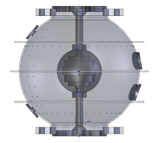
Figure 1: Sketch of the central part of the $DTS$ experiment. The $7.4\text{cm}$–radius inner sphere is made of copper and contains 5 layers of magnets. The inner radius of the stainless steel outer sphere is $21\text{cm}$ and its thickness is $5\text{mm}$. Blind holes are drilled and threaded along several meridians and parallels to receive electrodes. The large holes at latitudes $-20{{}^{\circ}}$, $10{{}^{\circ}}$ and $\pm 40{{}^{\circ}}$ receive interchangeable assemblies, which can be equipped with ultrasonic transducers.

symbol	expression	units	value
$a$	outer radius	cm	$21$
$b$	inner radius	cm	$7.4$
$\tau_{J}$	$a^{2}/\pi^{2}\eta$	s	$0.05$
			$\underline{\qquad B=B_{i}\qquad}$	$\underline{\qquad B=B_{o}\qquad}$
Ha	$aB/\sqrt{\mu_{0}\rho\nu\eta}$		4400	210
S	$aB/\eta\sqrt{\mu_{0}\rho}$		12	0.56
$U_{a}$	$B/\sqrt{\mu_{0}\rho}$	m s-1	5.1	0.2
			$\underline{\qquad f=5\text{Hz}\qquad}$
E	$\nu/\Omega a^{2}$		$4.7\;10^{-7}$
			$\underline{\>B=B_{i}\>}$	$\underline{\>B=B_{o}\>}$
$\Lambda$	$\sigma B^{2}/\rho\Omega$		9.2	0.02
$\lambda$	$U_{a}/a\Omega$		0.77	0.04
			$\underline{\qquad\Delta f=5\text{Hz}\qquad}$
$U$	$b\Delta\Omega$	m s-1	2.3
Rm	$Ua/\eta$		5.5
Re	$Ua/\nu$		$7\;10^{5}$
			$\underline{\>B=B_{i}\>}$	$\underline{\>B=B_{o}\>}$
N	$\sigma aB^{2}/\rho U$		26	0.006

Table 1: Typical values of the relevant parameters and dimensionless numbers for given imposed rotation frequencies $f=\Omega/2\pi$ of the outer sphere and differential rotation of the inner sphere $\Delta f=\Delta\Omega/2\pi$ with respect to the outer sphere. For the numbers that depend on the magnetic field strength, two values are given, the first one with $B=B_{i}=0.175$ T at the equator of the inner sphere, the second one with $B=B_{o}=0.008$ T at the equator of the outer sphere.

The radius of the outer sphere is $a=21$cm. Because of this moderate dimension, the Joule dissipation time $\tau_{J}$ of magnetic fluctuations by diffusion is small (less than one tenth of a second). The Alfvén wave velocity $U_{a}$ depends on the strength of the magnetic field, and is thus much stronger near the inner sphere than at the outer sphere. Comparing the Alfvén time to the diffusion time yields the Lundquist number S. It reaches $12$ on the inner sphere, suggesting that Alfvén waves can survive there, while they must be severely damped near the outer boundary, even though the Hartmann number Ha is large everywhere in the shell.

The rotation frequency $f$ of the outer sphere has been varied between $0$ and $15$Hz. The small value of the Ekman number for a typical rotation frequency of $5$Hz illustrates that the Coriolis force dominates over viscous forces in the bulk of the fluid. A very thin Ekman layer (one tenth of a millimeter) must form beneath the outer shell. The value of the Elsasser number $\Lambda$, which compares the Lorentz force to the Coriolis force, shows that rotation effects dominate in that region, while the opposite holds near the inner sphere. The domain of magnetostrophic equilibrium $\Lambda\simeq 1$ occupies the central part of the fluid shell. The number $\lambda$, called Lehnert number in [10], compares the frequencies of Alfvén modes to that of rotation (inertial) modes. It is smaller than $1$ everywhere.

Other effects depend upon the strength of the forcing, measured by $\Delta f$, the differential rotation frequency of the inner sphere with respect to the outer sphere. It can be varied between about $-20$Hz and $20$Hz. For a moderate value of $5$Hz, the expected fluid velocity $U$ is of the order of $2$m/s. The Reynolds number Re is thus very large, while the magnetic Reynolds number Rm is larger than $5$, indicating that the magnetic field is modified by the flow. The large value of the interaction parameter N near the inner sphere demonstrates that, in turn, the magnetic field deeply influences the flow.

The $DTS$ set–up is well suited for exploring the magnetostrophic regime. It is not a dynamo experiment, but the imposed magnetic field is strong enough to give rise to Lorentz forces of the same order as the Coriolis force. Both forces have a strong influence on the flow. The magnetic Reynolds number is large enough for induction effects to be well developed. We now examine what flow results from this complex combination, which is typical in planetary cores.

3 Characteristics of the mean axisymmetric flow

We use ultrasonic Doppler velocimetry to measure the mean axisymmetric flow. A transducer is placed in one of the interchangeable assemblies at latitude $10{{}^{\circ}}$, and shoots a beam with declination and inclination angles of $60{{}^{\circ}}$ and $66{{}^{\circ}}$, respectively. After a $38\text{cm}$–long linear trajectory, the beam hits the outer sphere at a latitude of about $-28{{}^{\circ}}$. Azimuthal velocities being more than 10 times larger than radial velocities, the along–beam measured velocity directly yields an angular velocity profile.

Such a profile is shown in figure 2 for $f\simeq 5\text{Hz}$ and $\Delta f\simeq 5\text{Hz}$. Starting from the beam entry point at latitude $10{{}^{\circ}}$, we see that the angular velocity rises regularly from a value of about $0.25\text{m/s}$, reaching an almost uniform plateau farther in the fluid, and increasing again to reach a maximum of $1.05\text{m/s}$ where the beam gets closest to the inner sphere. Comparing with axisymmetric numerical simulations, Nataf et al. [8] explain that the velocity bump near the inner sphere is a signature of the magnetic wind: the Elsasser number is large and the angular velocity isolines follow the magnetic field lines; the magnetic coupling between the rotating inner sphere and the liquid sodium is efficient. Away from that bump, the flow is geostrophic as the Elsasser number gets below $1$ (see Table 1). The geostrophic flow is driven by the magnetic torque that results from the shearing of the magnetic field lines and slowed down by friction in the Ekman layers beneath the outer sphere. This situation has been well studied by Kleeorin et al. [11], in the asymptotic limit of small Ekman, Rossby, Reynolds and Elsasser numbers. At small cylindrical radius $s$, the imposed magnetic field is large and friction in the Ekman layers of the outer sphere is weak. As a consequence, the shear must be very small in order for the magnetic torque to remain small enough to balance the friction torque: the fluid is in rigid body rotation. The regular decrease in angular velocity as one gets farther away from the inner sphere was predicted by Kleeorin et al. [11]: friction increases while the imposed magnetic field decreases, implying an increasing shear. It is important to realize that the flow is geostrophic, as a consequence of strong rotation, but entirely driven by magnetic forces. A modified Taylor state is achieved, where the magnetic torque on cylindrical tubes parallel to the axis of rotation only balances the (weak) friction in the Ekman boundary layers. Note that, under this mechanism, the induced toroidal magnetic field is expected to be larger in the external region, where shear is large, than in the region near the inner sphere, although the imposed magnetic field is much larger there.

We find similar profiles for all values of $\Delta f$ as long as the Rossby number $\text{Ro}=\Delta f/f$ remains smaller than a few units. A good quantitative fit between the theory and the measurements is achieved, when one takes into account that the Ekman layers become turbulent in the experimental conditions (see [8]). Therefore, we think that the same dynamics prevails for the very small Rossby numbers that characterize flow in the Earth’s core.

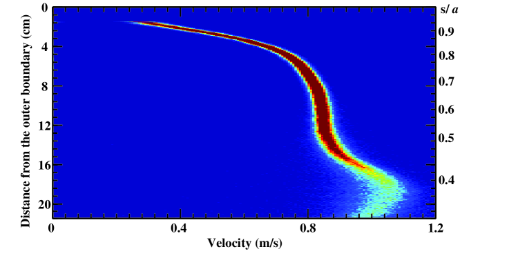
Figure 2: Profile of the angular velocity (velocity along the beam) of the flow as a function of distance from the outer sphere, obtained by ultrasonic Doppler velocimetry. The angular velocity rises smoothly to a plateau before it increases again as the ultrasonic beam gets closest to the inner sphere. $f\simeq 5\text{Hz}$ and $\Delta f\simeq 5\text{Hz}$. The (non–linear) scale on the right gives the value of the adimensional cylindrical radius $s$.

4 Weak turbulence

The profile shown in figure 2 is, in fact, a histogram constructed from over 1000 shots. Although the Reynolds number reaches $7\cdot 10^{5}$ for this run (see Table 1), the fluctuations around the average profile are amazingly small. Besides, the power spectra of the fluctuations reveal peculiar bumps at several frequencies. This is best seen on the spectrogram of a whole run, where $f\simeq 5\text{Hz}$ and $\Delta f$ is varied in steps from $0$ to $-20\text{Hz}$.

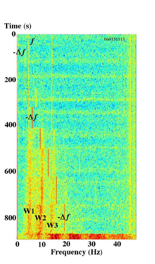
Figure 3: Spectrogram of electric potential measurement. The signal is the electric potential measured between two electrodes situated at latitude $-45{{}^{\circ}}$ and distant of $40{{}^{\circ}}$ in longitude. The colors give the log–amplitude of the short–time spectral density. The horizontal axis is frequency and the vertical axis is time. During this time–frame, the outer sphere was rotating at a constant angular frequency $f=5\text{Hz}$, while the inner sphere differential rotation rate $\Delta f$ was varied in steps from $0$ to $-20\text{Hz}$. The thin lines, labelled $f$ and $\Delta f$, reveal these frequencies and some overtones. The spectrum is almost void until $\Delta f$ reaches about $-10\text{Hz}$. The spectrum is then dominated by 3 broad bands (W1, W2, W3) whose frequency slightly decreases as $|\Delta f|$ increases.

Here, the signal is the difference in electric potential between two electrodes at the same latitude of $-45{{}^{\circ}}$ and distant of $40{{}^{\circ}}$ in longitude (see figure 1). The spectrogram is shown in figure 3. Frequency is on the horizontal axis and time on the vertical axis. The power spectral density of the signal is color–coded (log–scale). Thin lines reflect the two forcing frequencies $f$ and $-\Delta f$ and some overtones. For $-\Delta f<f$, the spectrum is featureless, while bands of higher power are clearly visible when $\Delta f$ reaches $-10\text{Hz}$. The detailed study of these bands performed by Schmitt et al [7] reveal that they correspond to waves that propagate in the direction of the flow (in the frame of reference rotating with the outer sphere) but at a slower velocity. The lowest band corresponds to a wave or mode with an azimuthal wave–number $m=1$, the following one to $m=2$, and so on. The origin of these waves is not clear yet. They are different from the inertial modes identified by Kelley et al [12] in a similar set–up but with a weak magnetic field. Indeed, the derivation of their dispersion relationship by Schmitt et al [7] reveal that their frequencies can be higher than that of inertial modes (which are bounded by $2f_{fluid}$, where $f_{fluid}$ is the rotation frequency of the fluid in the laboratory frame of reference).

Once again, useful information can be gained from ultrasonic Doppler velocity measurements. The bands that were first seen on power spectra of the induced magnetic field are also present in the power spectra of velocity, as illustrated in figure 4. They clearly extend deep into the sphere.

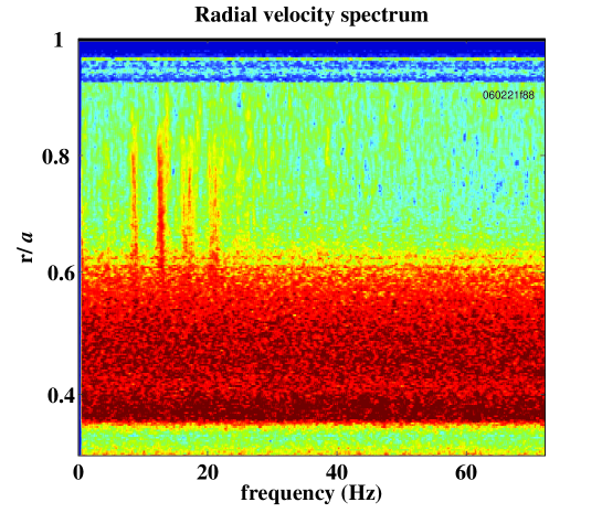
Figure 4: Radial profile of power spectral density of radial velocity versus frequency. Radial velocities are measured by ultrasonic Doppler velocimetry along a radial beam shot from a transducer at $-40{{}^{\circ}}$ in latitude. We then derive this image of color–coded log of power–spectral density as a function of adimensional radius $r/a$ and frequency. The rotation frequency of the sphere is $f=4.3\text{Hz}$ and the differential rotation frequency of the inner sphere is $\Delta f=-23\text{Hz}$. The power is high in bands at several frequencies, as in the spectrogram of figure 3.

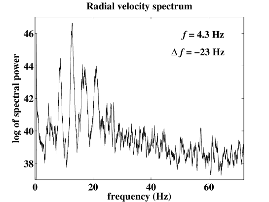
Figure 5: Power spectral density of radial velocity versus frequency at mid–depth. For the same record as in figure 4, we plot the log of power spectrum measured at mid–depth. Peaks at several frequencies dominate the spectrum.

We have seen that, in the modified Taylor state, the maximum induced toroidal field is not near the inner sphere. However, it is clear that a local perturbation of the azimuthal velocity near the inner sphere will induce a strong azimuthal magnetic field, which will in turn change the magnetic field and the torque that drives the azimuthal flow. It is tempting to see in this effect the origin of the waves we observe in $DTS$, but further work is needed to corroborate this hypothesis.

5 Implications for turbulence in the Earth’s core

Our experiments illustrate that, due to the strong influence of the Coriolis force, motions are geostrophic when the Elsasser number is less than 1, even though the magnetic torque on co–axial tubes is the only driving mechanism. Jault [10] argues that this property remains true even for large Elsasser numbers if one considers time scales that are short compared to the Alfvén time. Pais and Jault [13] apply this idea to retrieve geostrophic motions in the core that explain the observed secular variation of the magnetic field of the Earth between years 2000 and 2005.

The idea that motions are organized in cylinders around the axis of rotation dates back to Taylor [5]. He pointed out that, in the steady–state, the magnetic torque acting on such cylinders must vanish since, in the limit of small Ekman and Rossby numbers, there is no torque to balance it. The $DTS$ experiment supports this idea, with the modification that the magnetic torque is balanced by friction at the core–mantle boundary [11], and that this friction takes into account that the Ekman boundary layer becomes turbulent [8]. Although the local Reynolds number of the Ekman layers remain small in the core [14], enhanced friction at the core–mantle boundary can result from a rough boundary [15, 16], or from electromagnetic coupling between the core and the mantle [16]. In any case, nutation observations require a 10000–fold enhancement of core–mantle coupling, as compared to linear Ekman friction [17]. It would be worth it to take this effect into account in numerical simulations, in particular in quasi–geostrophic dynamo simulations [18], which are particularly efficient for exploring Earth–like fluid properties, and in which Ekman friction is already parameterized.

Our experiments also suggest that the only fluctuations left in the magnetostrophic regime, apart from localized turbulence in the Ekman layers, are waves that propagate azimuthally in a retrograde fashion. These global wave phenomena are usually excluded from the local turbulence analyses used to calibrate sub–grid algorithms in 3D numerical simulations [19]. This should probably be re–assessed once the origin of these waves is clearly established. In that respect, one should note one important limitation of our $DTS$ experiment: the time–scales that characterize the various kinds of waves are all very similar. For typical values of $f$ and $\Delta f$, the period of inertial waves and Alfvén waves, as well as the dissipation time of Alfvén waves are all of the order of $0.1\text{s}$. This makes it difficult to clearly identify the origin of the waves, and it prevents a complete exploration of the various regimes.

It was soon recognized that departures from the Taylor state would trigger a special kind of Alfvén waves, called torsional oscillations [20]. Assuming reasonable values for the –hidden– magnetic field within the core, the period of these waves should be of the order of 10 years. Both core flow models derived from the secular variation of the magnetic field [21] and numerical simulations of the geodynamo [22] have been explored in order to find evidence for these oscillations. The results indicate that part of the fluid motions could indeed be torsional oscillations, providing a nice link with the observed length–of–day variations [23]. However, recent analyses of the more precise satellite data also reveal large–scale motions that are not torsional oscillations. Regional “jerks” are thus observed by Olsen and Mandea [24], while the quasi–geostrophic core–flow models of Pais and Jault [13] are characterized by a large retrograde jet that is completely offset with respect to the axis of rotation, in violation of the axisymmetric character of torsional oscillations. All these observations, together with our detection of non–axisymmetric propagating waves in the $DTS$ experiment suggest to us that the importance of torsional oscillations in the Earth’s core could have been overemphasized. However, we should note again that, because the Alfvén time in our experiment is of the same order as the Joule dissipation time, torsional oscillations must be severely damped. It would be of great value to conduct experiments where Joule dissipation is less important.

Finally, we emphasize that fluctuations are very minute when the flow is under the combined influence of a strong magnetic field and rapid rotation (see figure 2 and 3). Basically, the flow is entirely constrained once the magnetic field and the rotation are given. When the Elsasser number is small, or when the timescale of the motions is short [10], the motions are constrained to be invariant along the rotation axis (quasi–geostrophy) but are driven by the Lorentz forces. As magnetic diffusion is small at short time–scales, only the flow can modify the magnetic field, and the same holds for the buoyancy field. One is thus led to conclude that the turbulence at work in planetary cores has little to do with classical turbulence. Our $DTS$ experiment is missing some of the key ingredients of a planetary dynamo, in fact it is not a dynamo. The $VKS$ experiment, which does behave as a dynamo [1], is also missing key ingredients of planetary dynamos: turbulence is almost entirely hydrodynamic and the produced magnetic field has a negligible effect on the flow. The mechanisms of the spectacular magnetic reversals observed in $VKS$ [2], as those of the pioneer experiments of Lowes and Wilkinson [25], probably have little to do with those at work in the Earth’s core.

6 Conclusion

Laboratory experiments such as our $DTS$ experiment help us better understand the peculiar organization of fluid flow and magnetic field at work in planetary dynamos. When the Coriolis and Lorentz forces are dominant, and the Elsasser number less than 1, a modified Taylor state is observed, where the geometry is given by the rotation (invariance along the axis of rotation) and the driving by the Lorentz force. In a Taylor state, the magnetic torque on co–axial tubes self–adjusts to zero, since there is no balancing torque. In our experiments, as foreseen by Kleeorin et al [11], Ekman friction at the external surface balances the magnetic torque. In this modified Taylor state, the flow remains geostrophic (azimuthal) and its variation with cylindrical radius is entirely controlled by the balance between the magnetic torque the resulting shear produces and the friction at the external boundaries. Using ultrasonic Doppler velocimetry, we measure time–averaged azimuthal velocity profiles in perfect agreement with this analysis.

Under the combined constraints of the imposed rotation and magnetic field, velocity fluctuations are very minute even though the Reynolds number is in the range $10^{6}$. When present, the fluctuations reveal a very peculiar behavior: the power spectra are dominated by peaks at several frequencies. The detailed analysis of the signals reveal that they correspond to waves that propagate in a retrograde fashion with respect to the fluid [7]. The spectral peaks correspond to various azimuthal wave numbers. It is not yet clear what are the driving forces of these magneto–inertial waves.

We infer that turbulence at work in planetary dynamos is of a very special kind: the flow is a complete slave of rotation and magnetic forces, Ekman friction at the boundaries providing a balancing torque. But the magnetic field itself is advected by the flow, and the same holds for the buoyancy field.

Two main limitations of the $DTS$ experiment prevent it of approaching regimes more relevant for planetary situations. The first one is that it is not a dynamo experiment, hence the magnetic field is not free to be advected by the flow. However, in most experimental dynamos, the produced magnetic field is too weak to substantially alter the flow, in contrast with what occurs in $DTS$. The second limitation is that all relevant time–scales (Alfvén, Joule dissipation, rotation, Rossby times) are in the same range (of order $0.1\text{s}$), in contrast with planetary situations. This makes it very difficult to isolate which are the main forces controlling the propagating waves we observe, and extrapolating to natural situations. Building an experiment exempt of these two limitations represents a tantalizing challenge, which has led Dan Lathrop and his group to build a promising 3m–diameter experiment in Maryland.

References

- [1] R. Monchaux, M. Berhanu, M. Bourgoin, Ph. Odier, M. Moulin, J.-F. Pinton, R. Volk, S. Fauve, N. Mordant, F. Pétrélis, A. Chiffaudel, F. Daviaud, B. Dubrulle, C. Gasquet, L. Marié, F. Ravelet, Generation of magnetic field by a turbulent flow of liquid sodium, Phys. Rev. Lett. 98 (2006) 044502.
- [2] M. Berhanu, R. Monchaux, S. Fauve, N. Mordant, F. Pétrélis, A. Chiffaudel, F. Daviaud, B. Dubrulle, L. Marié, F. Ravelet, M. Bourgoin, Ph. Odier, J.-F. Pinton, R. Volk, Magnetic field reversals in an experimental turbulent dynamo, European Phys. Lett. 77 (2007) 59001.
- [3] A. Gailitis, O. Lielausis, E. Platacis, S. Dement’ev, A. Cifersons, G. Gerbeth, T. Gundrum, F. Stefani, M. Christen, G. Will, Magnetic Field Saturation in the Riga Dynamo Experiment, Phys. Rev. Lett. 86 (2001) 3024-3027.
- [4] R. Stieglitz, U. and Müller, Experimental demonstration of a homogeneous two–scale dynamo, Phys. Fluids 13 (2001) 561-564.
- [5] J.B. Taylor, The magneto–hydrodynamics of a rotating fluid and the Earth’s dynamo problem, Proc. R. Soc. Lond. A 274 (1963) 274 -283.
- [6] H.-C. Nataf, T. Alboussière, D. Brito, P. Cardin, N. Gagnière, D. Jault, D. Schmitt, Experimental study of super–rotation in a magnetostrophic spherical Couette, Geophys. Astrophys. Fluid Dyn. 100 (2006) 281–298.
- [7] D. Schmitt, T. Alboussière, D. Brito, P. Cardin, N. Gagnière, D. Jault, H.-C. Nataf, Rotating spherical Couette ow in a dipolar magnetic eld: experimental study of magneto–inertial waves, J. Fluid Mech. 604 (2008) 175–197.
- [8] H.-C. Nataf, T. Alboussière, D. Brito, P. Cardin, N. Gagnière, D. Jault, D. Schmitt, Rapidly rotating spherical Couette flow in a dipolar magnetic field: an experimental study of the mean axisymmetric flow, Phys. Earth Planet. Inter., accepted (2008)
- [9] P. Cardin, D. Brito, D. Jault, H.-C. Nataf, J.-P. Masson, Towards a rapidly rotating liquid sodium dynamo experiment, Magnetohydrodynamics 38 (2002) 177-189.
- [10] D. Jault, Axial invariance of rapidly varying diffusionless motions in the Earth’s core interior, Phys. Earth Planet. Inter. 166 (2008) 67–76.
- [11] N. Kleeorin, I. Rogachevskii, A. Ruzmaikin, A.M. Soward, S. Starchenko, Axisymmetric flow between differentially rotating spheres in a dipolemagnetic field, J. Fluid Mech. 344 (1997) 213–244.
- [12] D.H. Kelley, S.A. Triana, D.S. Zimmerman, A. Tilgner, D.P. Lathrop, Inertial waves driven by differential rotation in a planetary geometry, Geophys. Astrophys. Fluid Dyn. 101 (2007) 469–487.
- [13] M.A. Pais, D. Jault, Quasi–geostrophic flows responsible for the secular variation of the Earth’s magnetic field, Geophys. J. Int. 173 (2008) 421–443.
- [14] B. Desjardins, E. Dormy, E. Grenier, Boundary layer instability at the top of the Earth’s outer core, J. Comput. Appl. Math. 166 (2004) 123–131.
- [15] J.-L. Le Mouël, C. Narteau, M. Grefftz-Lefftz, M. Holschneider, Dissipation at the core- mantle boundary on a small–scale topography, J. Geophys. Res. 111 (2006) B04413, doi:10.1029/2005JB003846.
- [16] B.A. Buffett, U.R. Christensen, Magnetic and viscous coupling at the core- mantle boundary: inferences from observations of the Earth’s nutations, Geophys. J. Int. 171 (2007) 145–152.
- [17] T.A. Herring, P.M. Mathews, B.A. Buffett, Modeling nutation and precession: very long baseline interferometry results, J. Geophys. Res. 107B (2002) doi:10.1029/2001JB000165.
- [18] N. Schaeffer, P. Cardin, Quasi–geostrophic kinematic dynamos at low magnetic Prandtl numbers, Earth Planet. Sci. Lett. 245 (2006) 595-604.
- [19] H. Matsui, B.A. Buffett, Commutation error correction for large eddy simulations of convection driven dynamos, Geophys. Astrophys. Fluid Dyn. 101 (2007) 429–449.
- [20] S.I. Braginsky, Torsional magnetohydrodynamic vibrations in the Earth s core and variations in day length, Geomag. Aeron. 10 (1970) 1- 8.
- [21] S. Zatman, J. Bloxham, Torsional oscillations and the magnetic eld within the Earth s core, Nature 388 (1997) 760–763.
- [22] M. Dumberry, J. Bloxham, Torque balance, Taylor s constraint and torsional oscillations in a numerical model of the geodynamo, Phys. Earth Planet. Int. 140 (2003) 29 -51.
- [23] D. Jault, C. Gire, J.-L. Le Mouël, Westward drift, core motions and exchanges of angular momentum between core and mantle, Nature 333 (1988) 353–356.
- [24] N. Olsen, M. Mandea, Investigation of a secular variation impulse using satellite data: the 2003 geomagnetic jerk, Earth Panet. Sci. Lett. 255 (2007) 94–105.
- [25] F.J. Lowes, I. Wilkinson, Geomagnetic dynamo: an improved laboratory model, Nature 219 (1968) 717–718.