Can we extract the pion electromagnetic form factor from a $t$-channel diagram only?

Abstract

We show that we are able to extract the pion electromagnetic form factor by using the recent charged pion electroproduction data from JLab and a simple $t$-channel diagram. For this purpose we have performed the $Q^{2}$-independent and dependent analyses. The result of the first analysis is in good agreement with those of previous works and fit the Maris and Tandy model as well as the monopole parameterization which describes a pion radius of 0.672 fm. The result of the second analysis corroborates the findings in the first analysis. Our findings therefore provide a direct proof that at the given kinematics the $t$-channel diagram really dominates the process. This could also set a new constraint to the phenomenological models that try to describe the process.
Keywords : Pion; electromagnetic form factor; electroproduction.
PACS : 14.40.Aq, 13.40.Gp, 25.30.Rw.

1 Introduction

In nuclear physics pions occupy a special place. Being the lightest meson in its family, pions play the major role in strong interaction. In fact, pions were the first mesons predicted by Yukawa as the mediator of the strong nuclear force. However, despite intensive investigations for decades, our understanding of the pion structure is far from complete. This is reflected, e.g., by the incomplete available data base of the pion electromagnetic form factor $F_{\pi}(Q^{2})$ in a considerably wide range of virtual photon momentum transfer $Q^{2}$. We understand that $F_{\pi}$ is nothing but a Fourier transformation of the charge distribution.

At very small $Q^{2}$ the behavior of $F_{\pi}$ has been accurately determined by scattering of high energy pions from atomic electrons [1]. At higher $Q^{2}$ values one should consult pion electroproduction off a nucleon.

With the continuous and excellent electron beams available at modern accelerators, such as CEBAF at JLab, it is now possible to measure pion electroproduction observables with unprecedented accuracy, at certain kinematics inaccessible with previous technology. This allows for a precise extraction of the longitudinal differential cross section via a Rosenbluth separation, at very small values of Mandelstam variable $-t$ [2, 3, 4]. These recent data show that the cross section $d\sigma/dt$ at this kinematics exhibit a steep decreasing function of $-t$, indicating the dominance of the $t$-channel contribution in the process. This behavior becomes the first pillar for the $F_{\pi}$ extraction in Refs. [2, 3, 4]. The extracted $F_{\pi}$ values within the range of $0.6\lesssim Q^{2}\lesssim 2.5$ GeV² are impressively accurate. Nevertheless, it is important to note that these extractions:

• rely heavily on the $t$-channel dominant assumption, although the assumption has never been directly checked.

• are model dependent. In Refs. [2, 3, 4] the Regge model of Ref. [5] has been utilized to obtain $F_{\pi}$.

• are plagued with the model uncertainties, which come from the extrapolation of the form factor cut-off to the physical limit. These uncertainties have been reported by Ref. [4].

• are “strategy” dependent. As shown in Ref. [4], by using the same data and model as in Ref. [2] but focusing the analysis on the minimal $t$ allowed by kinematics, where the unwanted background is assumed to be negligible, smaller $F_{\pi}$ values are obtained.

The above facts indicate that current extraction methods are far from established. Since a completely model-independent extraction is quite difficult and challenging (although it is not impossible, see Ref. [6] for instance), attempts in this direction would be invaluable for helping to resolve this issue.

It is the purpose of this paper to revisit a simple method, à la Chew-Low, which is based only on the first assumption. This will also serve as an alternative method, which is obviously easy to check.

This paper is organized as follows. In Section 2 we briefly describe the formalism used in our calculation. Section 3 presents the result of the $Q^{2}$-independent analysis, where we extract the electromagnetic form factor for fixed $Q^{2}$ values. Section 4 demonstrates the result of the $Q^{2}$-dependent analysis, i.e., the result when we parameterize the form factor with a monopole form and fit all available data simultaneously. We shall summarize and conclude our findings in Section 5.

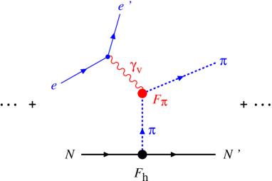
Figure 1: (Color online) The $t$-channel diagram that dominates the contributions to the pion electroproduction process. The electromagnetic and hadronic form factors are denoted by $F_{\pi}$ and $F_{\rm h}$, respectively.

2 Formalism

We begin with the convention of four-momenta given in the process

$$\gamma_{v}(k)+N(p)\to\pi(q)+N(p^{\prime})~{},$$ (1)

to write the $t$-channel amplitude for the diagram shown in Fig. 1 as [7, 8]

$${\cal M}=\left[\frac{2ieg_{\pi NN}F_{\pi}(k^{2})F_{\rm h}(t)}{k^{2}(t-m_{\pi}^{2})}\right]{\bar{u}}(p^{\prime})\gamma_{5}(k^{2}q\cdot\epsilon-k\cdot qk\cdot\epsilon)u(p),$$ (2)

where $e$ is the proton charge, $\epsilon$ denotes the virtual photon polarization, while $m_{\pi}$ and $g_{\pi NN}$ are the pion mass and the pion-nucleon coupling constant, respectively.

In Eq. (2) the hadronic and electromagnetic form factors are denoted by $F_{\rm h}$ and $F_{\pi}$, respectively, while the Mandelstam variable $t$ can be written as

$$t=(k-q)^{2}=k^{2}+m_{\pi}^{2}-2k\cdot q~{}.$$ (3)

Note that in Eq. (2) we have added the so-called the Fubini-Nambu-Wataghin term [8] in order to retain the gauge invariance [9].

Clearly, this amplitude contributes only to the longitudinal cross section. For meson electroproduction it is well known that this cross section can be written as [10]

$$\frac{d\sigma_{\rm L}}{d\Omega}=\frac{-2|\vec{q}|Wk^{2}}{(s-m^{2})k_{0}^{2}}~{}\Bigl{[}|f_{5}|^{2}+|f_{6}|^{2}+2\cos\theta{\rm Re}(f_{5}^{*}f_{6})\Bigr{]},$$ (4)

where $W$ indicates the total c.m. energy, $\theta$ is the pion scattering angle, and

$$f_{5,6}=\mp\frac{k_{0}}{8\pi W}\left(\frac{E^{\prime}\pm m}{E\pm m}\right)^{1/2}(q\cdot kk_{0}-q_{0}k^{2})A_{5}~{},$$ (5)

with $m$ denotes the nucleon mass and $A_{5}$ is given by the term inside the square bracket in the r.h.s. of Eq. (2). Inserting Eq. (5) into Eq. (4) and by making use of

$$\frac{d\sigma_{L}}{dt}~{}=~{}\frac{\pi}{|\vec{k}|\,|\vec{q}|}\,\frac{d\sigma_{L}}{d\Omega}~{},$$ (6)

we obtain

$$\frac{d\sigma_{L}}{dt}=t\,\frac{e^{2}g_{\pi NN}^{2}k^{2}F_{\pi}^{2}(k^{2})F_{\rm h}^{2}(t)}{8\pi W(s-m^{2})(t-m_{\pi}^{2})^{2}|\vec{k}|^{3}}\left(q_{0}-\frac{k\cdot q}{k^{2}}k_{0}\right)^{2}.$$ (7)

Since we are working with small $t$, we can neglect both $t$ and $m_{\pi}$ in Eq. (3) to obtain $k^{2}\approx 2k\cdot q$, so that the last term of Eq. (7) can be reduced to $(q_{0}-\frac{1}{2}k_{0})$. This has an advantage, because we have reduced the dependencies of the cross section on $t$. Finally, we can shift the pion propagator term to the l.h.s. of Eq. (7) and using $Q^{2}=-k^{2}$ to obtain

$$(t-m_{\pi}^{2})^{2}\frac{d\sigma_{L}}{dt}=-t\,\frac{e^{2}g_{\pi NN}^{2}Q^{2}F_{\pi}^{2}(Q^{2})F_{\rm h}^{2}(t)}{8\pi W(s-m^{2})|\vec{k}|^{3}}\,\left(q_{0}-{\textstyle\frac{1}{2}}k_{0}\right)^{2}~{}.$$ (8)

The r.h.s. of Eq. (8) were a linear function of $t$, if we could neglect the hadronic form factor $F_{\rm h}$. If this were the case, then an extrapolation of Eq. (8) to the pion pole ($t=m_{\pi}^{2}$) could be directly performed to determine the $F_{\pi}$ at a certain $Q^{2}$ value, because the r.h.s. is free of poles and the extrapolation (setting $t$ at $m_{\pi}^{2}$) will eliminate other contributions beyond the $t$-channel one. However, as we clearly understand, this is not the case.

To overcome the shortcoming of the extrapolation method, here we only assume that Eq. (8) is valid in the physical region ($t<0$, but still small) because the $t$-channel dominates the process. Thus, for each value of $Q^{2}$, Eq. (8) can be fitted to the data in the form of

$$y=F_{\pi}^{2}\cdot f(t)+g~{},$$ (9)

to obtain $F_{\pi}$. In Eq. (9) we introduce the $g$ parameter to account for other terms neglected in Eq. (8). Obviously, the use of this parameter improves the $\chi^{2}$ significantly, thus, absorbing more information from the electroproduction data, but at the cost of increasing the flexibility of the fit, i.e., increasing the error bars of the extracted $F_{\pi}$.

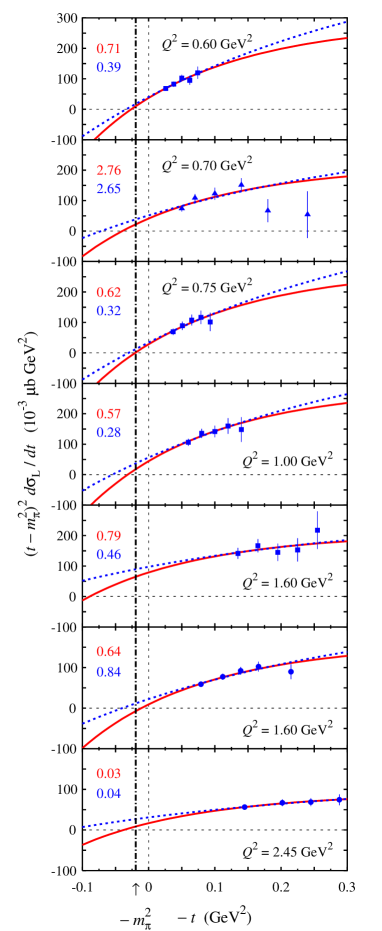
Figure 2: (Color online) The modified longitudinal differential cross section as a function of the Mandelstam variable $-t$. Solid (dotted) lines show the results of fitting to experimental data with $\Lambda_{\rm h}=0.85~{}(1.30)$ GeV. Solid squares [4] and solid circles [3] show the recent JLab data, whereas solid triangles display the older data from DESY [19]. The upper (lower) numbers at the left part of each panel show the values of $\chi^{2}/N$ obtained for $\Lambda_{\rm h}=0.85~{}(1.30)$ GeV.

3 $Q^{2}$-Independent Analysis

In this analysis we first fix the value of the pion-nucleon coupling constant to be $g_{\pi NN}^{2}/(4\pi)=14.17$ [11]. We note that in the literature this value varies from 13.45 [12] to 14.52 [13]. Thus, our choice lies nicely in this range. Later, we will also try to investigate the influence of the coupling constant variation on the extracted form factor. For the hadronic vertex we adopt the monopole form factor

$$F_{\rm h}(t)=\left(1-\frac{t}{\Lambda_{\rm h}^{2}}\right)^{-1}~{}.$$ (10)

Reference [14] has pointed out that $\Lambda_{\rm h}=0.85$ GeV is generally used, whereas the precise value of $\Lambda_{\rm h}$ is a matter of controversy and may vary between 0.4 and 1.5 GeV. Meson exchange models for nucleon-nucleon interaction dictates that $\Lambda_{\rm h}\gtrsim 1.30$ GeV [15], whereas lattice QCD calculations prefer a value of 0.75 GeV [16]. On the other hand QCD sum rule calculations yield $\Lambda_{\rm h}=0.80$ GeV [17], while K. Vansyoc [18] found that $\Lambda_{\rm h}\lesssim 1.00$ GeV is demanded by the present pion electroproduction data.

In this work we found that the best result is obtained by using $\Lambda_{\rm h}=1.30$ GeV, i.e., the case when we consider the result of meson exchange models for the nucleon-nucleon interactions [15]. Nevertheless, using the generally accepted value (i.e. $\Lambda_{\rm h}=0.85$ GeV) the obtained result is still in good agreement with previous analyses.

At $W=1.95$ GeV there are four sets of data points from Ref. [4] with $Q^{2}=0.6$, 0.75, 1.00 and 1.60 GeV², as a function of $t$. At higher energy and momentum transfers ($W=2.22$ GeV, $Q^{2}=1.6$ and 2.45 GeV²), two more data sets are available from Ref. [3]. For the sake of comparison, we also present the reanalyzed DESY data at $W=2.19$ GeV, $Q^{2}=0.70$ GeV² [19]. These data were fitted separately by using the CERN-MINUIT code. A combination of the simplex and migrad packages has been used [20]. The fitted (modified) cross sections are shown in Fig. 2, where we can see that, except for the DESY data, the $\chi^{2}/N$ values obtained from the fits are quite encouraging.

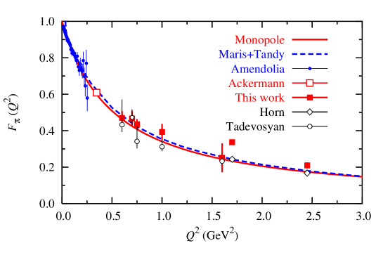
Figure 3: (Color online) The electromagnetic form factors of pion extracted in this work and previous calculations. The monopole form factor is obtained by using the pion charge radius of 0.672 fm (PDG value [21]). The dashed line shows the model of Maris and Tandy [22]. Results of the present work are obtained by using $\Lambda_{\rm h}=0.85$ GeV and shown in this figure by the solid (red) squares. Other data shown here are from Amendolia et al. [1], Ackermann et al. [23], Horn et al. [3], and Tadevosyan et al. [4]. The data point of Horn et al. at 1.6 GeV, as well as the corresponding result of the present analysis, have been slightly shifted for visual clarity.

The extracted $F_{\pi}$ for $\Lambda_{\rm h}=0.85$ GeV and 1.30 GeV compared with the results of previous calculations are listed in Table 1 and depicted in Fig. 3. The error bars reported here are also obtained from MINUIT. Their magnitudes can be easily understood from the comparison between the fit results (solid and dashed lines) and the experimental data as demonstrated in Fig. 2.

Table 1: Values of the extracted $F_{\pi}$ in the $Q^{2}$-independent analysis obtained by using $\Lambda_{\rm h}=0.85$ GeV and 1.30 GeV compared with those of previous works. Reference [4] has reported “model uncertainties” listed as the second error-bars in the fourth column.

$Q^{2}$	$F_{\pi}$ (this work)		$F_{\pi}$ (previous works)
(GeV2)	$\Lambda_{\rm h}=0.85$ GeV	$\Lambda_{\rm h}=1.30$ GeV
0.60	$0.470\pm 0.037$	$0.438\pm 0.066$	$0.433\pm 0.017^{+0.137}_{-0.036}$ [4]
0.70	$0.467\pm 0.041$	$0.395\pm 0.076$	$0.473\pm 0.023^{+0.038}_{-0.034}$ [4]
0.75	$0.435\pm 0.028$	$0.396\pm 0.088$	$0.341\pm 0.022^{+0.078}_{-0.031}$ [4]
1.00	$0.393\pm 0.044$	$0.341\pm 0.074$	$0.312\pm 0.016^{+0.035}_{-0.019}$ [4]
1.60	$0.251\pm 0.079$	$0.194\pm 0.124$	$0.233\pm 0.014^{+0.013}_{-0.010}$ [4]
1.60	$0.337\pm 0.009$	$0.276\pm 0.036$	$0.243\pm 0.012$ [3]
2.45	$0.209\pm 0.017$	$0.153\pm 0.042$	$0.167\pm 0.010$ [3]

Figure 3 reveals that, within the error bars, our simple analysis results in a good agreement with previous analyses [3, 4]. At first glance the error bars obtained in the present work would seem to be much larger than those of previous works. However, this is in general not true. For example, consider the case of $Q^{2}=0.6$ GeV². By combining the error bar obtained in Ref. [4] with the reported error bar coming from the “model uncertainty” we can clearly see that the error bar of the present work is indeed smaller. For other cases the error bars of the present work are mostly comparable to those of previous analysis. Only at $Q^{2}=1.60$ GeV² the obtained error bar is much larger. The reason behind this behavior is obvious from Fig. 2. Comparing with the result of Ref. [3] at the same kinematics we can conclude that this error bar can be significantly reduced if more statistics are available at this point.

The two data points at 1.6 and 2.45 GeV² from Ref. [3] require a special explanation. First, Ref. [3] does not report the “model uncertainties” which appear during the extraction process. From Table 1 we can see that these uncertainties are substantial in increasing the error bars [4]. Second, the discrepancy appears between our result and those of Ref. [3] for these two data points are presumably due to higher $W$ and $t$, where other terms excluded in Eq. (8) could start to contribute. Nevertheless, the error bars for the two $F_{\pi}$ at $Q^{2}=1.6$ GeV² of our results indicate that our analysis in this case is still consistent. Therefore, we believe that the error-bars obtained in the present work are realistic, especially if we compare them with those obtained from scattering of high energy pions from atomic electrons at $Q^{2}\approx 0.25$ GeV² [1]. Thus, more statistics in the longitudinal cross section data will reduce these values.

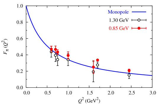
Figure 4: (Color online) The influence of the variation of the hadronic form factor cut-off $\Lambda_{\rm h}$ on the extracted pion electromagnetic form factor. The monopole form factor is as in Fig. 3.

In Fig. 4 we demonstrate the variation of the extracted electromagnetic form factor $F_{\pi}$ due to the variation of the hadronic cut-off ($\Lambda_{\rm h}=0.85$ GeV and 1.30 GeV). The corresponding numerical values for the two cases are listed in Table 1. A soft cut-off will substantially suppress the cross section. To overcome this suppression the fit will increase the electromagnetic form factor cut-off. This explains why the extracted $F_{\pi}$ values increase once we decrease the hadronic cut-off. From this figure we may conclude that the best agreement with the results of Refs. [3, 4] is obtained if we set the hadronic cut-off to $1.3$ GeV, a case when we consider the result of meson exchange models for the nucleon-nucleon interactions [15].

Note that in Figs. 3 and 4 we compare our results with the monopole form factor obtained by using the Particle Data Group (PDG) value [21] of the pion charge radius, i.e. 0.672 fm. In the literature one can find that the value ranges from 0.560 fm [24] to 0.740 fm [25], whereas the recent Chiral Perturbation Theory extraction yields a value of 0.661 fm [26].

4 $Q^{2}$-Dependent Analysis

In the previous section we have extracted the electromagnetic pion form factors at fixed $Q^{2}$ values. It is however possible to analyze the whole experimental data simultaneously in a fit. For this purpose, we have to assume that the electromagnetic form factor can be parametrized with a monopole form factor,

$$F_{\pi}(Q^{2})=\left(1+\frac{Q^{2}}{\Lambda_{\pi}^{2}}\right)^{-1}~{}.$$ (11)

A quick glance to Fig. 4 indicates that with this monopole parameterization it would be difficult to produce the pion charge radius as reported by PDG, especially if we used $\Lambda_{\rm h}=0.85$ GeV, for which we see that the two extracted form factors at $Q^{2}=1.6$ GeV² and 2.45 GeV² obviously overestimate the monopole parameterization. For $\Lambda_{\rm h}=1.30$ GeV we could expect that such a parameterization would still fairly work, since as shown in Fig. 4 the PDG form factor is still within the corresponding error bars.

Nevertheless, a simultaneous fit to all available experimental data is quite important if we want to investigate the internal consistency of the data or the general trend of the extracted parameters. Furthermore, within this framework we can leave the fit to determine not only the electromagnetic form factors $F_{\pi}$, but also the hadronic cut-off $\Lambda_{\rm h}$ and the pion-nucleon coupling constant $g_{\pi NN}$. Here, it is important to note that compared to the conventional approaches, which make use of thousands data points, a simultaneous fit to only 36 data points is clearly less reliable to accurately determine the hadronic cut-off and coupling constant of the pion. Therefore, our motivation here is only to confirm the results obtained by the $Q^{2}$-independent analysis given in the previous section as well as to check our claim about the limitation of our model.

Table 2: Values of some important parameters extracted from fit to three different sets of experimental data in the $Q^{2}$-dependent analysis. References for the literature are given in the text.

Parameter	All data (36 points)	19 Data points	18 Data points	Literature†
$\langle r_{\pi}^{2}\rangle^{1/2}$ (fm)	$0.576\pm 0.020$	$0.596\pm 0.111$	$0.625\pm 0.272$	0.560 - 0.740
$g$	$0.019\pm 0.006$	$0.022\pm 0.013$	$0.025\pm 0.007$	-
$\Lambda_{\rm h}$ (GeV)	$0.850\pm 0.034$	$0.968\pm 0.256$	$1.300\pm 0.230$	0.400 - 1.500
$g_{\pi NN}^{2}/(4\pi)$	$14.500\pm 0.827$	$14.500\pm 0.623$	$14.500\pm 0.721$	13.45 - 14.52
$\chi^{2}/N$	1.118	0.348	0.263	-
†See text.

As a first step, we fit all experimental data by leaving the pion charge radius $\langle r_{\pi}^{2}\rangle^{1/2}$ (for the sake of comparison, instead of the $\Lambda_{\pi}$), the constant $g$ in Eq. (9), the hadronic cut-off $\Lambda_{\rm h}$, and the coupling constant $g_{\pi NN}$, as free parameters. Since we only intent to qualitatively study the extracted parameters, we limit the pion charge radius in the range of 0.560 fm - 0.740 fm, the hadronic cut-off between 0.85 GeV and 1.30 GeV, and the pion-nucleon coupling constant $g_{\pi NN}^{2}/(4\pi)$ between 13.50 and 14.50. The corresponding numerical values extracted from this fit along with their $\chi^{2}/N$ are shown in the second column of Table 2. The individual $\chi^{2}$ as a function of $t$ is plotted in Fig. 5. Fitting to all available data results in a total $\chi^{2}$ of about 36. Interestingly, we found that more than 36% of it come from the reanalyzed DESY data at $W=2.19$ GeV, $Q^{2}=0.70$ GeV² [19]. This indicates that these data are probably incompatible with the recent JLab data [3, 4]. Furthermore, we found that these data belong also to the high-$t$ and $W$ data.

The more surprising result is however shown by the set of the new JLab data at $Q^{2}=2.45$ GeV² [3]. Although this data set contains five precise data points, the combination of high $t$, $W$, and $Q^{2}$, obviously puts these data beyond the limitation of our approach. For $Q^{2}=0.60$ GeV² only the data point at $|t|=0.06$ GeV² yields $\chi^{2}>1$. This is understandable if we look at the first panel of Fig. 2, where it is obvious that this data point slightly underestimates the trend of the other data. The same situation happens for the last data point at $Q^{2}=0.75$ GeV². Finally, we found that the first two data points at $Q^{2}=1.00$ GeV² and $Q^{2}=1.60$ GeV² overestimate the fit result. This fact is relatively difficult to explain, especially for the first case, for which the corresponding $t$ are clearly small. Probably, these data points are too high or other physics beyond our approach at this kinematics are missing.

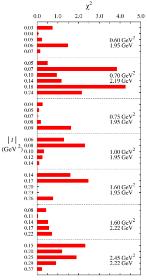
Figure 5: (Color online) Values of the $\chi^{2}$ obtained from fit to all experimental data in the $Q^{2}$-dependent analysis plotted as a function of $|t|$. Note that the two numbers given in each panel show the corresponding values of $Q^{2}$ and $W$, respectively. The order of the experimental data sets shown in this figure (from top to bottom) is as in Fig. 2.

As a second step we remove the data points that produce $\chi^{2}>1$ from our fitting data base. The number of data points at this step turns out to be 19. The extracted parameters obtained from fitting to these data are shown in the third column of Table 2. Obviously the $\chi^{2}/N$ decreases significantly. The pion charge radius and hadronic cut-off increase slightly from those of the first fit, whereas the pion coupling stays the same. The only interesting result at this step is the fact that the highest $\chi^{2}$ comes from the data point at $W=2.22$ GeV, $Q^{2}=1.60$, $|t|=0.22$ GeV². Again, this is understandable because of the combination of high $t$ and $W$ and, furthermore, this data point seems to underestimate the trend of other four data points.

As the last step we remove the data point at $W=2.22$ GeV, $Q^{2}=1.60$, $|t|=0.22$ GeV² from our fitting data base and refit the rest of the data (18 points). The extracted parameters for this step are shown in the fourth column of Table 2. The value of $\chi^{2}/N$ is very small, indicating that our approach works pretty well for these selected data. The pion charge radius (as well as its error bar) and the hadronic cut-off increase significantly after we have removed the last data point as described above. Although having a relatively large error bar, the pion charge radius is now much closer to the PDG value compared to those obtained in the first and second steps. Thus, the result of the third step corroborates the finding in the $Q^{2}$-independent analysis, i.e., smaller $\chi^{2}$ values would be obtained if we used $\Lambda_{\rm h}=1.30$ GeV. Another way to understand this result is by comparing the electromagnetic form factors $F_{\pi}$ obtained from this analysis with that of the PDG and those obtained from the $Q^{2}$-independent analysis described in the previous section. This is shown in Fig. 6, where we can clearly see that omitting the high-$\chi^{2}$ data (put in other words, using experimental data with the kinematics allowed by the model) results in a form factor that is in closer agreement with the form factor of PDG and those obtained from the $Q^{2}$-independent analysis with $\Lambda_{\rm h}=1.30$ GeV.

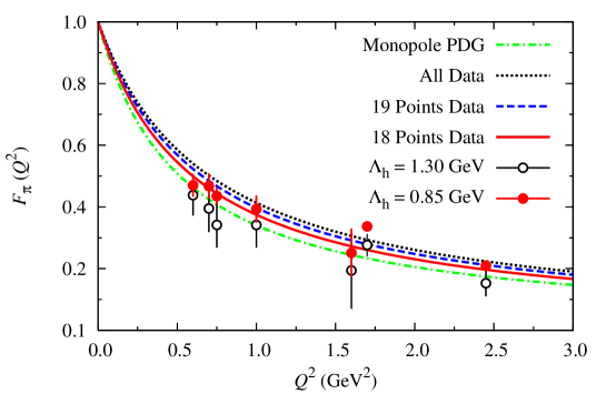
Figure 6: (Color online) Electromagnetic form factors of the pion according to the results of fitting to three different sets of experimental data in the $Q^{2}$-dependent analysis. The corresponding pion charge radii are listed in Table 2. For comparison, results of the $Q^{2}$-independent analysis with $\Lambda_{\rm h}=0.85$ GeV and 1.30 GeV are also shown by the solid and open circles, respectively.

It is also important to note that the values of $g$ and pion coupling constant are relatively stable for the three different fits (see Table 2). The relatively large error bars for the latter indicate that our conclusion drawn from the two analyses is not too sensitive to the variation of the $g_{\pi NN}$ within the fit limit.

5 Conclusion

In conclusion, we would like to say that we are able to extract the electromagnetic form factor of pion from the recent longitudinal cross section data of pion electroproduction from JLab by using a simple $t$-channel diagram, which utilizes fewer assumptions compared to the previous calculations. For this purpose we have performed a $Q^{2}$-independent analysis supplemented with a $Q^{2}$-dependent analysis. The result of the first analysis shows a good agreement with $F_{\pi}$ extracted from previous works. The extracted values depend on the choice of the hadronic form factor cut-off. Nevertheless, by using the generally accepted value we still obtain a satisfactory result. The best result would be obtained if we used a cut-off from the meson exchange model. The result of the second analysis corroborates the findings of the first one. More accurate, with also smaller $|t|$, longitudinal cross section data will certainly help to reduce the uncertainty of the present calculation. Finally, we would like to mention that this simple calculation provides for the first time a direct proof that at the given kinematics pion electroproduction is dominated by the $t$-channel process. Previous works considered this merely as an assumption. This result could set a new constraint on the phenomenological models that try to explain the process, i.e. at the kinematics given in this paper contributions from other channels should vanish or a least should be minimal. We note that, however, at small $t$ but higher energies, contributions of certain resonances to the process could be substantial.

References

- [1] S. R. Amendolia et al., Nucl. Phys. B 277, 168 (1986); Phys. Lett. B 138, 454 (1984).
- [2] J. Volmer et al., Phys. Rev. Lett. 86, 1713 (2001).
- [3] T. Horn et al., Phys. Rev. Lett. 97, 192001 (2006).
- [4] V. Tadevosyan et al., Phys. Rev. C 75, 055205 (2007).
- [5] M. Vanderhaeghen, M. Guidal, and J.-M. Laget, Phys. Rev. C 57, 1454 (1998); Nucl. Phys. A 627, 645 (1997).
- [6] B. B. Deo and A. K. Bisoi, Phys. Rev. D 13, 1927 (1976).
- [7] J. D. Bjorken and S. D. Drell, Relativistic Quantum Mechanics (Mc Graw-Hill, New York, 1964).
- [8] S. Fubini, Y. Nambu, and V. Wataghin, Phys. Rev. 111, 329 (1958).
- [9] The procedure to maintain gauge invariance is briefly discussed in Ref. [10]. Another recipe is given by Haberzettl in H. Haberzettl, Phys. Rev. C 56, 2041 (1997). This recipe yields also the same result (H. Haberzettl, private communication). An application to meson photoproduction is discussed in H. Haberzettl, C. Bennhold, T. Mart, and T. Feuster, Phys. Rev. C 58, R40 (1998).
- [10] B. B. Deo and A. K. Bisoi, Phys. Rev. D 9, 288 (1974).
- [11] T. E. O. Ericson, B. Loiseau, and A. W. Thomas, Phys. Rev. C 66, 014005 (2002); I. G. Aznauryan, Phys. Rev. C 67, 015209 (2003).
- [12] R. G. E. Timmermans, Newslett. 13, 80 (1997).
- [13] J. Rahm et al., Phys. Rev. C 57, 1077 (1998).
- [14] J. Volmer, Ph.D. Thesis, Vrije Universiteit, Amsterdam, 2000 (available at http://www.jlab.org/Hall-C), p. 12.
- [15] R. Machleidt et al., Phys. Rept. 149, 1 (1987).
- [16] K.-F Liu, S.-J. Dong, T. Draper, and W. Wilcox, Phys. Rev. Lett. 74, 2172 (1995)
- [17] T. Meissner, Phys. Rev. C 52, 3386 (1995).
- [18] K. Vansyoc, Ph.D. Thesis, Old Dominion University, 2001 (available at http://www.jlab.org/Hall-C).
- [19] P. Brauel et al., Z. Phys. C 3, 101 (1979).
-
[20]
F. James, “MINUIT, Function Minimization and Error Analysis,
Reference Manual Version 94.1”, available online via:
http://wwwasdoc.web.cern.ch/wwwasdoc/minuit/minmain.html. - [21] W.-M. Yao et al., J. Phys. G 33, 1 (2006).
- [22] P. Maris and P. C. Tandy, Phys. Rev. C 62, 055204 (2000).
- [23] H. Ackermann et al., Nucl. Phys. B 137, 294 (1978).
- [24] E. B. Dally et al., Phys. Rev. Lett. 39, 1176 (1977).
- [25] A. Liesenfeld et al., Phys. Lett. B 468, 20 (1999).
- [26] J. Bijnens, G. Colangelo, and P. Talavera, JHEP 9805, 014 (1998).