Abstract

We report results of the investigation of gap solitons (GSs) in the generic model of a periodically modulated Bragg grating (BG), which includes periodic modulation of the BG chirp or local refractive index, and periodic variation of the local reflectivity. We demonstrate that, while the previously studied reflectivity modulation strongly destabilizes all solitons, the periodic chirp modulation, which is a novel feature, stabilizes a new family of double-peak fundamental BGs in the side bandgap at negative frequencies (gap No. $-1$), and keeps solitons stable in the central bandgap (No. $0$). The two soliton families demonstrate bistability, coexisting at equal values of energy. In addition, stable 4-peak bound states are formed by pairs of fundamental GSs in bandgap $-1$. Self-trapping and mobility of the solitons are studied too.

OCIS codes: (060.5530) Pulse propagation and solitons; (230.1480) Bragg reflectors.

1 Introduction and the model

The technology for writing grating superstructure (alias superlattices) on optical fibers had become available twenty years ago [1, 2]. These superlattices are Bragg gratings (BGs) with a long-wave modulation of period $\sim 1$ mm imposed on them, while the underlying BG period is $\lambda/2\lesssim 1$ $\mu$m ($\lambda$ is the wavelength of light coupled into the BG). A theoretical model shows that, in addition to the central bandgap generated by the underlying uniform BG, the superstructure gives rise to a new set of bandgaps [3]. In this connection, it is relevant to mention that the modulation of the periodic lattice potential in the Schrödinger equation, produced by beatings between two lattices with close periods, also gives rise to additional narrow “mini-gaps” in the respective spectrum [4]. Taking into regard the Kerr nonlinearity of the fiber, as in the theory of gap solitons (GSs) in the uniform fiber BG [7, 5, 6], “coupled-supermode” equations were derived in Ref. [3], and examples of the corresponding GSs were found (these equations bear a similarity to coupled-mode equations for deep BGs [8, 9]). Stable solitons in the above-mentioned mini-gaps of the Gross-Pitaevskii equation with the repulsive cubic nonlinearity, which is a model of the Bose-Einstein condensate (BEC) trapped in the optical lattice, were found too [4]. Another example of the superstructure was developed in the form of the Moiré pattern, with a sinusoidal modulation imposed on the periodic variation of the refractive index underlying the ordinary BG. The Moiré supergrating features a narrow transmission band in the middle of the central gap, which was proposed [10, 11] and realized experimentally [12] as a means for the retardation of light in gratings.

Cellular optical media which resemble the BG structure and may also be used as a basis for the design of superstructures are CROWs (coupled resonant optical waveguides) [13, 14]. It is also possible to realize superstructure patterns in the recently proposed “semi-discrete” BG (a waveguide with uniform nonlinearity and periodically distributed short segments with strong Bragg reflectivity) [15]. A vast potential for the synthesis of complex grating patterns is offered by techniques developed for writing BGs in photonic crystals and photonic-crystal fibers [16, 17, 18].

A topic of fundamental significance is families of GSs and their stability in models describing superstructured BGs. In fact, the stability of GSs is a nontrivial issue even in the standard model of uniform BGs [19, 20, 21]). A basic system of coupled-mode equations for counterpropagating waves $u(x,t)$ and $v(x,t)$ in the periodically modulated BG was proposed in Ref. [22]. In the normalized form, it is

$$i\frac{\partial u}{\partial t}+i\frac{\partial u}{\partial x}+\left[1-\varepsilon\cos\left(kx\right)\right]v+\mu\cos\left(kx\right)\cdot u+\left(\left|v\right|^{2}+\frac{1}{2}\left|u\right|^{2}\right)u = 0,$$

$$i\frac{\partial v}{\partial t}-i\frac{\partial v}{\partial x}+\left[1-\varepsilon\cos\left(kx\right)\right]u+\mu\cos\left(kx\right)\cdot v+\left(\left|u\right|^{2}+\frac{1}{2}\left|v\right|^{2}\right)v = 0.$$

Here, $\varepsilon$ is the amplitude of the modulation of the Bragg reflectivity (in other words, it represents periodic apodization of the grating [23]), while $\mu$ admits two interpretations: it accounts for the periodic variation of the local chirp of the BG [24, 22], or of the effective refractive index of the carrying fiber. The spatial period of both modulations is $2\pi/k$. We define the model by fixing $\mu>0$, while $\varepsilon$ may take zero, positive, and negative values.

It is known that GSs are possible not only as temporal solitons in fiber gratings, but also as spatial solitons in planar waveguides equipped with the grating in the form of a system of parallel grooves [25, 26, 27, 28], as well as solitons in photonic crystals [29]. Equations (LABEL:CME) may also be interpreted in that context (replacing $t$ by propagation coordinate $z$), with $\mu$ representing the amplitude of a long-wave longitudinal modulation of the refractive index in a layered planar waveguide.

The results obtained in this work are presented in Section II, where families of soliton solutions and their stability are reported, and in Section III, which deals with the self-trapping and nonlinear evolution of stable and unstable GSs, and with moving solitons. In the previously studied model of the reflectivity modulation [22], the GSs quickly become unstable with the increase of modulation amplitude $\varepsilon$. In Section II we demonstrate that the effect of the periodic modulation of the local chirp (or refractive index) – a feature that was not studied before – is different: a part of the GS family filling out the central bandgap (labeled as gap $0$ below, see Fig. 1) remains stable with the increase of $\mu$, while the first side bandgap emerging at $\omega<0$ (designated below as gap $-1$) supports a new partially stable family of fundamental GSs, whose characteristic feature is a two-peak shape, unlike the ordinary single-peak solitons existing in the central bandgap (in bandgap $+1$, GSs also feature the double-peak shape, but they are unstable). Note that fundamental GSs in the Gross-Pitaevskii equation with a periodic potential do not feature a dual-peak structure. In terms of the spatial-domain model, the double-peak solitons may find an application as optically induced conduits routing weak signal beams [28]. In Section III it is shown that, in the model with $\varepsilon=0$ and $\mu>0$, stable quiescent solitons belonging to the central gap readily self-trap from moving input pulses of a general form, hence the periodically chirp-modulated BG may serve as a tool for the creation of solitons of standing-light.

Unlike the standard BG model, in the present system stable double- and single-peak solitons, residing in gaps $-1$ and $0$, respectively, feature bistability, coexisting at equal values of energy. 4-peak bound states of two double-peak solitons, and 3-peak complexes, built of three single-peak solitons, may be stable too (recall that bound states of GSs do not exist in the standard BG).

In Section III we demonstrate that the evolution of unstable GSs in the modulated system features another novelty: unstable solitons with a sufficiently large energy self-retrap into stable double-peak GSs belonging to bandgap $-1$, while unstable GSs do not transform themselves into stable ones in the standard model. Other unstable GSs evolve into persistent breathers, or may be destroyed by the instability. In Section III we also study a possibility to set quiescent GSs in motion, which is suggested by the fact that, thus far, BG solitons in fiber gratings have been created only at finite velocity $c$; in the first works, it was $c\geq 0.5$ [with respect to the largest velocity in Eqs. (LABEL:CME), $c_{\max}=1$] [30, 31], while later it was brought down to $c\approx 0.23$ [32]. In terms of the above-mentioned spatial-domain interpretation, moving solitons correspond to tilted beams. We demonstrate that stable moving solitons are supported by Eqs. (LABEL:CME) with $\varepsilon=0$ and small values of $\mu$. In fact, these results also stress that the modulated BG offers a possibility to bring moving pulses to a halt and thus create solitons of standing light.

2 Stationary solutions and their stability

2.1 The mode of the analysis

Stationary solutions of Eqs. (LABEL:CME) with frequency $\omega$ and zero velocity are looked for as $\left\{u\left(x,t\right),v\left(x,t\right)\right\}=\left\{U\left(x\right),V\left(x\right)\right\}\exp\left(-i\omega t\right)$, with complex functions $U$ and $V$ satisfying equations

$$+i\frac{dU}{dx}+\left[\omega+\mu\cos\left(kx\right)\right]U+\left[1-\varepsilon\cos\left(kx\right)\right]V+\left[\left(\left|V\right|^{2}+\frac{1}{2}\left|U\right|^{2}\right)\right]U=0,$$

(2)

$$-i\frac{dV}{dx}+\left[\omega+\mu\cos\left(kx\right)\right]V+\left[1-\varepsilon\cos\left(kx\right)\right]U+\left[\left(\left|U\right|^{2}+\frac{1}{2}\left|V\right|^{2}\right)\right]V=0.$$

For the numerical solution, the complex amplitudes were split into real and imaginary parts, $\left\{U(x),V(x)\right\}\equiv\left\{U_{1}(x),V_{1}(x)\right\}+i\left\{U_{2}(x),V_{2}(x)\right\}$, and the resulting system of four equations was solved by means of the Newton’s iteration method. The initial guess generating even solutions was $U_{10}\left(x\right)=U_{20}\left(x\right)=V_{10}\left(x\right)=V_{20}\left(x\right)=A~{}\mathrm{sech}\left(ax\right)$, with constants $A$ and $a$.

Numerical results are reported below for $k=1$, which represents the generic situation. Families of soliton solutions are characterized by the total energy (on total power, in terms of the spatial-domain model),

$$E=\int_{-\infty}^{+\infty}\left(\left|u\right|^{2}+\left|v\right|^{2}\right)dx,$$ (3)

to be presented as a function of $\omega$.

The bandgap spectrum of the linearized version of Eqs. (2) was computed by means of software package SpectrUW [33]. The spectra are displayed in Fig. 1, which also show stability borders of GS families found in the bandgaps from the solution of the full nonlinear system, as described below. Note that the region occupied by bandgap $-1$ in Fig. 1(b) (for $\varepsilon=0.5$) splits into two parts, with stable solitons existing only in the upper one.

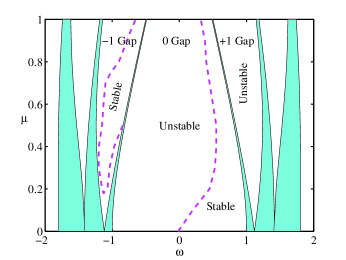
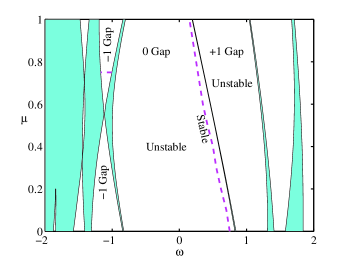
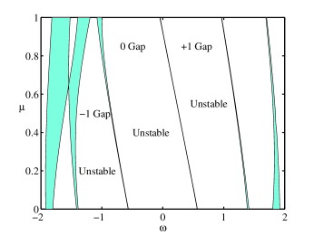
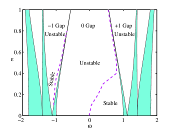
Fig. 1: The bandgap structure found from the linearization of Eqs. (2) for (a) $\varepsilon=0$, (b) $\varepsilon=0.5$, (c) $\varepsilon=1$ and (d) $\mu=0$. Shaded areas are occupied by Bloch bands. Five gaps are displayed: the central one (No. $0$) and two side bandgaps, $\pm 1$ and $\pm 2$ (gaps $\pm 2$ are not labeled). Stable solitons are found in gaps $0$ and $-1$, where borders between stability and instability areas are shown by dashed lines. Note that all solitons are unstable for $\varepsilon=1$.

The linearization of Eqs. (2) is invariant with respect to transformation $\varepsilon\rightarrow-\varepsilon$, $\omega\rightarrow-\omega$, $x\rightarrow x+\pi/k$, $\left\{U,V\right\}\rightarrow\left\{-V,U\right\}$; therefore, the linear spectrum for $\varepsilon<0$ can be obtained as a mirror image (with $\omega\rightarrow-\omega$) from its counterpart for $-\varepsilon$. However, this transformation does not apply to full nonlinear equations (2). On the other hand, Eqs. (2) admit the reduction to a single equation by means of the well-known substitution, $V=\pm U^{\ast}$. As well as in the standard model, the GSs found in the central bandgap satisfy “ordinary” reduction $V=-U^{\ast}$, while double-peak solitons populating bandgap $-1$ (and unstable solitons of the same type in bandgap $+1$) obey the “extraordinary” reduction, $V=U^{\ast}$.

Stability of solitons was identified by dint of simulations of the evolution of perturbed solitons, typically up to $t=10,000$, which means several thousand soliton periods, or time $\sim 1$ ns, in physical units. It was additionally checked, in typical cases, that the solutions which are identified as stable ones retain their stability in arbitrarily long simulations. The simulations were performed by means of the split-step Fourier-transform method, with absorbers placed at edges of the integration domain. The domain was covered by a mesh consisting of $N=\allowbreak 512$ grid points, and the stepsize of the time integration was $\Delta t=0.01$ (it was checked that further increase of $N$ and decrease of $\Delta t$ did not alter the results).

Figure 1 clearly shows that the increase of the reflectively modulation, represented by $\varepsilon$, quickly destabilizes all solitons. On the other hand, the model with the periodic chirp modulation, which is accounted for by $\mu$ (unlike the system with $\varepsilon>0$, it was not studied before), supports stable GSs, including the new family in gap $-1$. Therefore, we focus below on the study of this model; some new results for the case of $\mu=0$ and $\varepsilon\neq 0$ will be included too, for the sake of comparison.

2.2 Results

In addition to Fig. 1, the stability of the GSs is summarized in Fig. 2, which displays typical dependences $E(\omega)$ [recall $E$ is defined in Eq. (3)] for soliton families in several generic cases and in different bandgaps (situations where all solitons are unstable, such as at $\varepsilon=1$, are not included). As said above, stable solitons are found only in bandgaps $0$ and $-1$. For instance, the stability intervals in gaps $-1$ and $0$ for $\mu=0.5$ and $\varepsilon=0$ are $-1.17<\omega<-0.84$ and $0.55<\omega<0.82$, respectively. If the existence range of gap $-1$ splits into two parts, as in Fig. 1(b), stable solitons are found only in the upper one [in Fig. 1(b), the stability area in bandgap $-1$ is located at $\mu>0.75$)]. A notable feature observed in Figs. 2(a,c) is the bistability: stable portions of the GS families in gaps $0$ and $-1$ may cover identical intervals of energy. In higher-order bandgaps, starting from $\pm 2$, all GSs are unstable.

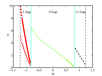
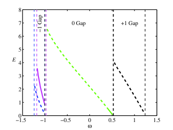
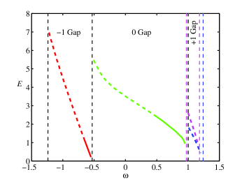
Fig. 2: Gap-soliton families, shown in the form of energy $E$ versus intrinsic frequency $\omega$, for (a) $\mu=0.5$, $\varepsilon=0$, (b) $\mu=\varepsilon=0.5$, (c) $\mu=-\varepsilon=0.5$. Stable and unstable portions of the families are depicted by continuous and dashed lines, respectively. The upper bold curve in gap $-1$ in (a) represents the family of 4-peak bound states of fundamental solitons. Two different curves in (b) and (c), in gaps $-1$ and $+1$, respectively, pertain to two regions in which these gaps exist, cf. Fig. 1(b). Recall that, for $\varepsilon<0$ [as in (c)], the bandgap structure is obtained from that for $-\varepsilon$ as the mirror image, with $\omega\rightarrow-\omega$.

A characteristic feature of the GSs in bandgap $-1$ is the double-peak shape, as shown in Fig. 3(a). We stress that the double-peak GSs are fundamental solitons, rather than bound states of some single-peak pulses. Note that all GSs in bandgap $-1$ have a single peak in the model with $\mu=0$ and $\varepsilon>0$ [22] [and almost all of them are unstable, see Fig. 1(d)]. As mentioned above, the solitons in gap $-1$obey the “extraordinary” reduction, $V=U^{\ast}$. Unlike them, in gap $0$ GSs are similar to their counterparts in the standard model, being subject to the ordinary reduction, $V=-U^{\ast}$, see Fig. 3(b).

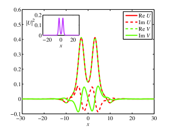
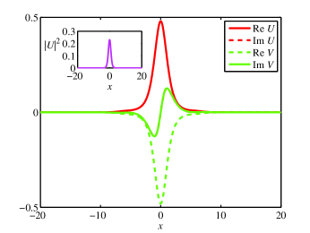
Fig. 3: (a) A stable double-peak soliton found in gap $-1$, for $\mu=0.5$, $\varepsilon=0$, and $\omega=-1$. The energy of this soliton is $E=1.83$. (b) A stable single-peak soliton in gap $0$, for $\mu=0.5$, $\varepsilon=0$, and $\omega=0.6$. Its energy is $E=0.96$.

Unlike the GSs in the central bandgap, which do not combine into bound states, solitons in bandgap $-1$ may form several species of complexes, symmetric and anti-symmetric ones. Only one of them is stable, viz., a 4-peak symmetric bound state of two double-peak solitons, see an example in Fig. 4(a). The entire family of such states is shown in Fig. 2(a) by the upper bold curve. The conclusion that the 4-peak states are bound states of fundamental solitons is clearly suggested by the comparison of curves $E(\omega),$ which shows that the energy of the 4-peak structure is, approximately, twice that of the double-peak soliton at the same $\omega$. The stability area of the 4-peak states is identical to that of the fundamental GSs. In addition, stable 3-peak symmetric bound states of three single-peak solitons were found in that small part of gap $-1$ in the model with $\varepsilon\neq 0$ and $\mu=0$ where the GSs are stable as per Fig. 1(d), see an example in Fig. 4(b) (bound states were not studied in Ref. [22]).

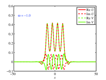
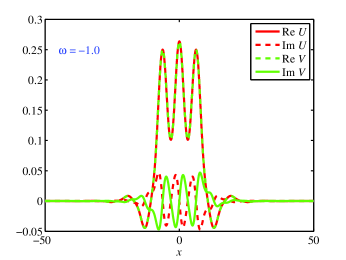
Fig. 4: (a) A stable bound state of two fundamental twin-peak solitons in gap $-1$, for $\mu=0.5$, $\varepsilon=0$, and $\omega=-1.0$. The energy of this state is $3.76$, while the energy of each constituent soliton is $1.83$. (b) A stable bound state of three single-peak solitons for $\mu=0$, $\varepsilon=0.3$, and $\omega=-1$. The energy of the bound state is $1.30$, the energy of each constituent being $0.35$.

3 Nonlinear evolution of stable and unstable solitons

3.1 Self-trapping of stable solitons

To appraise the experimental relevance of the GSs, it is necessary to consider the possibility of self-trapping of such solitons from standard input pulses (Gaussians). In the fiber BG, the input always has a finite velocity, and, obviously, it may contain only a single (forward) component. In the spatial-domain setting, the input beams may be both straight and tilted (the former one corresponds to zero velocity in the temporal domain), and simultaneous coupling of both components into the grating is possible.

Simulations demonstrate that stable quiescent single-peak solitons in the central bandgap can be readily produced by self-trapping of the one-component moving input pulses, see a typical example in Fig. 5. In this figure, the velocity of the input pulse is $c=0.2$ (recall $c=1$ is the largest normalized velocity possible in the model). Faster inputs generate stable standing solitons with more conspicuous intrinsic oscillations. It is relevant to mention that the creation of solitons of “standing light” in fiber BGs is a challenging problem (previously elaborated theoretical scenarios for that relied on the retardation provided by a smooth apodization [34], and the fusion of colliding solitons into standing ones [35]).

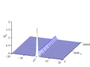
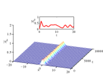
Fig. 5: Self-trapping of an input pulse of the forward wave ($u$), at initial velocity $c=0.2$, into a quiescent ($c=0$) soliton with residual internal vibrations, which falls into the central bandgap, in the model with $\mu=0.5$ and $\varepsilon=0$. The inset in (b) illustrates the initial growth of field $v$, which is absent in the input, at the soliton’s center. The energy of the input pulse is $E=2.28$, of which $40\%$ is kept by the established soliton.

Double-peak GSs belonging to bandgap $-1$ cannot be formed from single-component inputs, even if the input pulse itself is given a dual-peak shape. However, they can easily self-trap from moving two-component single-peak Gaussians, as shown in Fig. 6, in the model with $\mu>0$ and $\varepsilon=0$. On the other hand, even small nonzero values of $\varepsilon$, if added to this model, make the self-trapping of the double-peak GSs impossible. This observation stresses, once again, that the periodic modulation of the chirp (or local refractive index), represented by $\mu$, generates robust fundamental GSs in gap $-1$, while the reflectivity modulation, accounted for by $\varepsilon$, strongly destabilizes them. As mentioned above, the use of the two-component input is possible in terms of the spatial-BG model.

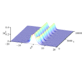
Fig. 6: Self-trapping of a two-component input pulse, moving at velocity $c=0.2$, into a standing double-peak soliton, in the model with $\mu=0.5$ and $\varepsilon=0$. This case is relevant to the spatial-domain model, see text. The input energy is $E=3.04$, about $60\%$ of which is kept by the emerging double-peak soliton.

3.2 The evolution of unstable solitons

In the standard BG model, unstable GSs (actually, those with $\omega<0$) transform themselves into persistent breathers, but they do not demonstrate re-trapping into stable GSs with a smaller energy. In the present system, the same is observed as a result of the evolution of unstable solitons in bandgaps $0$ and $+1$ (not shown here).

In gap $-1$, unstable solitons with a relatively low energy demonstrate a more violent instability, which may end up with the formation of a breather at a position different from that of the original unstable soliton, as shown in Fig. 7(a). On the other hand, unstable GSs with high energy in gap $-1$ feature an evolution scenario which does not occur in the standard model, viz., spontaneous rearrangement into another stable soliton belonging to the same bandgap. A typical example of such evolution is displayed in Fig. 7(b). Unstable double-peak solitons with still higher energies, which belong to gap $-2$, also self-retrap into stable two-peak GSs falling into bandgap $-1$.

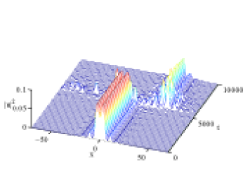
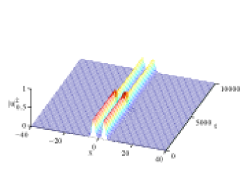
Fig. 7: (a) Formation of a breather from an unstable double-peak soliton in gap $-1$, for $\mu=0.1$, $\varepsilon=0$ and $\omega=-1.12$, $E=2.05$. Note the leap of the breather from the original position. (b) The transformation of an unstable double-peak soliton, with $\mu=0.9$, $\varepsilon=0$, $\omega=-1.1$ and $E=5$, into a stable gap soliton of the same type, with energy $E=3.3$. In (a) and (b), only the $u$ component is shown, as the evolution of field $v$ is quite similar.

3.3 Moving solitons

As mentioned above, only moving solitons have been observed in experiments performed in fiber BGs thus far [30, 31, 32]. This fact makes it necessary to study the mobility of stable solitons in the present model. This was done in the usual way, by applying a kick to stable quiescent solitons, i.e., multiplying them by $\exp\left(ic_{0}x\right)$.

The double-humped GSs found in gap $-1$ cannot be set in a state of persistent motion – they either pass a finite distance and come to a halt, or get destroyed, if the kink is too strong. On the other hand, stable single-peak solitons, originally belonging to the central bandgap, can move at a finite velocity, in the model with $\varepsilon=0$ and small amplitude of the chirp/refractive index modulation, $\mu\lesssim 0.03$ (moving solitons practically cannot be created in the model with $\mu=0$ and $\varepsilon\neq 0$ [22]) .

To display a generic example of the soliton mobility in the present system, we notice that, at $\mu=0.03$, the soliton with energy $E=3.00$ remains pinned if the kick is small, $c_{0}\leq 0.3$. At $c_{0}=0.31$, the kicked soliton performs several oscillations and then depins itself, starting progressive motion, as shown in Fig. 8. In this case, the velocity of the eventual steady motion is found to be $0.12\approx\allowbreak 0.4c_{0}$.

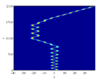
Fig. 8: Depinning of a soliton with energy $E=3.00$, which belongs to the central bandgap ($\omega=0.40$) in the model with $\mu=0.03$ and $\varepsilon=0$, by the kick with $c_{0}=0.31$, (this value only slightly exceeds the depinning threshold). The motion of the soliton is shown by means of contour plots of $|u|^{2}$.

In interval $0.3<c_{0}<0.45$, the same soliton readily sets in persistent motion, with average velocity $\bar{c}$ which is found to be slightly larger than $c_{0}/2$ (for example, $\bar{c}=0.19$ for $c_{0}=0.35$). A still stronger kick sends the soliton in motion for a limited (although long) interval of time, but then it suddenly gets destroyed by accumulated disturbances. In the latter case, the velocity observed at the stage of the quasi-stable motion is much lower than in the truly stable situation, $\bar{c}\approx 0.2c_{0}$. On the other hand, if the modulation strength increases to $\mu=0.05$, kicked GSs do not start to move, but rather demonstrate oscillations around the pinned state, up to $c_{0}\simeq 0.4$. A stronger kick destroys them.

4 Conclusion

We have reported results of systematic investigation of GSs (gap solitons) and their moving counterparts in the basic model of periodically modulated BGs (Bragg gratings), which includes periodic variations of the grating’s chirp (or local refractive index) and reflectivity. In addition to fiber BGs, the model may also be interpreted in terms of spatial gratings. The increase of the reflectivity modulation quickly makes all solitons unstable; on the other hand, the modulation of the chirp supports a new species of stable BGs in the side bandgap at negative frequencies (gap No. $-1$), and keeps solitons stable in the central bandgap, No. $0$. The characteristic feature of the GSs in the side bandgaps is their double-peak shape. The stable single- and double-peak solitons in gaps $0$ and $-1$, respectively, demonstrate bistability, existing in overlapping intervals of the energy. Stable 4-peak bound complexes, formed in bandgap $-1$ by the double-peak fundamental GSs, were found too.

Quiescent single-peak solitons belonging to the central bandgap readily self-trap from one-component input pulses, which are launched into the BG at a finite velocity, while the GSs in gap $-1$ self-trap from the bimodal input, which is relevant to spatial gratings. On the other hand, unstable two-peak solitons with a large energy, belonging to bandgaps $-1$ and $-2$, spontaneously re-trap into stable double-peak GSs (spontaneous rearrangement of unstable solitons into stable ones does not occur in the standard BG model). Moving solitons can be created in the BG with the weak chirp modulation.

The fabrication of the periodically modulated fiber gratings, considered in the present model, is quite feasible, and available experimental techniques should be sufficient for the creation of solitons predicted in this work. In particular, such experiments may bring closer a solution to the challenging problem of the creation of solitons made of standing light.

Acknowledgements

The work of T.M. is supported, in a part, by a postdoctoral fellowship from the Pikovsky-Valazzi Foundation, by the Israel Science Foundation through the Center-of-Excellence grant No. 8006/03, and by the Thailand Research Fund under grant No. MRG5080171.