INSTITUT NATIONAL DE RECHERCHE EN INFORMATIQUE ET EN AUTOMATIQUE

Parallel Pricing Algorithms
for Multi–Dimensional Bermudan/American Options
using Monte Carlo methods
Viet_Dung Doan — Abhijeet Gaikwad — Mireille Bossy — Françoise Baude — Ian Stokes-Rees N° 6530
Mai 2008

Abstract: In this paper we present two parallel Monte Carlo based algorithms for pricing multi–dimensional Bermudan/American options. First approach relies on computation of the optimal exercise boundary while the second relies on classification of continuation and exercise values. We also evaluate the performance of both the algorithms in a desktop grid environment. We show the effectiveness of the proposed approaches in a heterogeneous computing environment, and identify scalability constraints due to the algorithmic structure.

Key-words: Multi–dimensional Bermudan/American option, Parallel Distributed Monte Carlo methods, Grid computing.

Algorithmes de Pricing parallèles pour des Options Bermudiennes/Américaines multidimensionnelles par une méthode de Monte Carlo

Résumé : Dans ce papier, nous présentons deux algorithmes de type Monte Carlo pour le pricing d’options Bermudiennes/Américaines multidimensionnelles. La premiere approche repose sur le calcul de la frontière d’exercice, tandis que la seconde repose sur la classification des valeurs d’exercice et de continuation. Nous évaluons les performances des algorithmes dans un environnement grille. Nous montrons l’efficacité des approches proposées dans un environnement hétérogène. Nous identifions les contraintes d’évolutivité dues à la structure algorithmique.

Mots-clés : options Bermudiennes/Américaines multidimensionnelles, Méthodes de Monte Carlo paralléles, Grid computing.

1 Introduction

Options are derivative financial products which allow buying and selling of risks related to future price variations. The option buyer has the right (but not obligation) to purchase (for a call option) or sell (for a put option) any asset in the future (at its exercise date) at a fixed price. Estimates of the option price are based on the well known arbitrage pricing theory: the option price is given by the expected value of the option payoff at its exercise date. For example, the price of a call option is the expected value of the positive part of the difference between the market value of the underlying asset and the asset fixed price at the exercise date. The main challenge in this situation is modelling the future asset price and then estimating the payoff expectation, which is typically done using statistical Monte Carlo (MC) simulations and careful selection of the static and dynamic parameters which describe the market and assets.

Some of the widely used options include American option, where the exercise date is variable, and its slight variation Bermudan/American (BA) option, with the fairly discretized variable exercise date. Pricing these options with a large number of underlying assets is computationally intensive and requires several days of serial computational time (i.e. on a single processor system). For instance, Ibanez and Zapatero (2004) [10] state that pricing the option with five assets takes two days, which is not desirable in modern time critical financial markets. Typical approaches for pricing options include the binomial method [5] and MC simulations [6]. Since binomial methods are not suitable for high dimensional options, MC simulations have become the cornerstone for simulation of financial models in the industry. Such simulations have several advantages, including ease of implementation and applicability to multi–dimensional options. Although MC simulations are popular due to their “embarrassingly parallel" nature, for simple simulations, allows an almost arbitrary degree of near-perfect parallel speed-up, their applicability to pricing American options is complex[10], [4], [12]. Researchers have proposed several approximation methods to improve the tractability of MC simulations. Recent advances in parallel computing hardware such as multi-core processors, clusters, compute “clouds", and large scale computational grids have also attracted the interest of the computational finance community. In literature, there exist a few parallel BA option pricing techniques. Examples include Huang (2005) [9] or Thulasiram (2002) [15] which are based on the binomial lattice model. However, a very few studies have focused on parallelizing MC methods for BA pricing [16]. In this paper, we aim to parallelize two American option pricing methods: the first approach proposed in Ibanez and Zapatero (2004) [10] (I&Z) which computes the optimal exercise boundary and the second proposed by Picazo (2002) [8] (CMC) which uses the classification of continuation values. These two methods in their sequential form are similar to recursive programming so that at a given exercise opportunity they trigger many small independent MC simulations to compute the continuation values. The optimal strategy of an American option is to compare the exercise value (intrinsic value) with the continuation value (the expected cash flow from continuing the option contract), then exercise if the exercise value is more valuable. In the case of I&Z Algorithm the continuation values are used to parameterize the exercise boundary whereas CMC Algorithm classifies them to provide a characterization of the optimal exercise boundary. Later, both approaches compute the option price using MC simulations based on the computed exercise boundaries.

Our roadmap is to study both the algorithms to highlight their potential for parallelization: for the different phases, our aim is to identify where and how the computation could be split into independent parallel tasks. We assume a master-worker grid programming model, where the master node splits the computation in such tasks and assigns them to a set of worker nodes. Later, the master also collects the partial results produced by these workers. In particular, we investigate parallel BA options pricing to significantly reduce the pricing time by harnessing the computational power provided by the computational grid.

The paper is organized as follows. Sections 2 and 3 focus on two pricing methods and are structured in a similar way: a brief introduction to present the method, sequential followed by parallel algorithm and performance evaluation concludes each section. In section 4 we present our conclusions.

2 Computing optimal exercise boundary algorithm

2.1 Introduction

In [10], the authors propose an option pricing method that builds a full exercise boundary as a polynomial curve whose dimension depends on the number of underlying assets. This algorithm consists of two phases. In the first phase the exercise boundary is parameterized. For parameterization, the algorithm uses linear interpolation or regression of a quadratic or cubic function at a given exercise opportunity. In the second phase, the option price is computed using MC simulations. These simulations are run until the price trajectory reaches the dynamic boundary computed in the first phase. The main advantage of this method is that it provides a full parameterization of the exercise boundary and the exercise rule. For American options, a buyer is mainly concerned in these values as he can decide at ease whether or not to exercise the option. At each exercise date $t$, the optimal exercise point $S_{t}^{*}$ is defined by the following implicit condition,

$$P_{t}(S_{t}^{*})=I(S_{t}^{*})$$ (1)

where $P_{t}(x)$ is the price of the American option on the period $[t,T]$, $I(x)$ is the exercise value (intrinsic value) of the option and $x$ is the asset value at opportunity date $t$. As explained in [10], these optimal values stem from the monotonicity and convexity of the price function $P(\cdot)$ in (1). These are general properties satisfied by most of the derivative securities such as maximum, minimum or geometric average basket options. However, for the problems where the monotonicity and convexity of the price function can not be easily established, this algorithm has to be revisited. In the following section we briefly discuss the sequential algorithm followed by a proposed parallel solution.

2.2 Sequential Boundary Computation

The algorithm proposed in [10] is used to compute the exercise boundary. To illustrate this approach, we consider a call BA option on the maximum of $d$ assets modeled by Geometric Brownian Motion (GBM). It is a standard example for the multi–dimensional BA option with maturity date $T$, constant interest rate $r$ and the price of this option at $t_{0}$ is given as

$P_{t_{0}}=\mathbb{E}\left(\exp{(-r\tau)}\Phi(S_{\tau},\tau)|S_{t_{0}}\right)$

where $\tau$ is the optimal stopping time $\in\{t_{1},..,T\}$, defined as the first time $t_{i}$ such that the underlying value $S_{\tau}$ surpasses the optimal exercise boundary at the opportunity $\tau$ otherwise the option is held until $\tau=\infty$. The payoff at time $\tau$ is defined as follows: $\Phi(S_{\tau},\tau)=(\max_{i}(S^{i}_{\tau})-K)^{+}$, where $i$ = 1,..,$d$, $S$ is the underlying asset price vector and $K$ is the strike price. The parameter $d$ has a strong impact on the complexity of the algorithm, except in some cases as the average options where the number of dimensions $d$ can be easily reduced to one. For an option on the maximum of $d$ assets there are $d$ separate exercise regions which are characterized by $d$ boundaries [10]. These boundaries are monotonic and smooth curves in $\mathbb{R}^{d-1}$. The algorithm uses backward recursive time programming, with a finite number of exercise opportunities $m={1,...,N_{T}}$. Each boundary is computed by regression on $J$ numbers of boundary points in $\mathbb{R}^{d-1}$. At each given opportunity, these optimal boundary points are computed using $N_{1}$ MC simulations. Further in case of an option on the maximum of $d$ underlying assets, for each asset the boundary points are computed. It takes $n$ iterations to converge each individual point. The complexity of this step is $\mathbb{O}\left(\sum_{m=1}^{N_{T}}d\times J\times m\times N_{1}\times(N_{T}-m)\times n\right)$. After estimating $J$ optimal boundary points for each asset, $d$ regressions are performed over these points to get $d$ execution boundaries. Let us assume that the complexity of this step is $\mathbb{O}(N_{T}\times regression(J))$, where the complexity of the regression is assumed to be constant. After computing the boundaries at all $m$ exercise opportunities, in the second phase, the price of the option is computed using a standard MC simulation of $N$ paths in $\mathbb{R}^{d}$. The complexity of the pricing phase is $\mathbb{O}(d\times N_{T}\times N)$. Thus the total complexity of the algorithm is as follows,

$\mathbb{O}\left(\sum_{m=1}^{N_{T}}d\times J\times m\times N_{1}\times(N_{T}-m)\times n+N_{T}\times regression(J)+d\times N_{T}\times N\right)$

$\approx\mathbb{O}\left(N_{T}^{2}\times J\times d\times N_{1}\times n+N_{T}\times(J+d\times N)\right)$

For the performance benchmarks, we use the same simulation parameters as given in [10]. Consider a call BA option on the maximum of $d$ assets with the following configuration.

$$\begin{array}[]{l}\mbox{$K=100$, {interest rate r = 0.05}, {volatility rate $\sigma$ = 0.2},}\\ \mbox{{dividend $\delta$ = 0.1}, $J=128$, $N_{1}=5e3$, $N=1e6$, $d=3$, }\\ \mbox{$N_{T}=9$ and $T=3$ years.}\end{array}$$ (5)

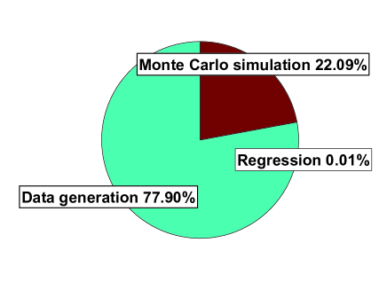
Figure 1: The time distribution for the sequential optimal exercise boundary computation algorithm. The total time is about 40 minutes.

The sequential pricing of this option (5) takes 40 minutes. The distribution of the total time for the different phases is shown in Figure 1. As can be seen, the data generation phase, which simulates and calculates $J$ optimal boundary points, consumes most of the computational time. We believe that a parallel approach to this and other phases could dramatically reduce the computational time. This inspires us to investigate a parallel approach for I&Z Algorithm which is presented in the following section. The numerical results that we shall provide indicate that the proposed parallel solution is more efficient compared with the serial algorithm.

2.3 Parallel approach

In this section, a simple parallel approach for I&Z Algorithm is presented and the pseudocode for the same is given in Algorithm 13. This approach is inspired from the solution proposed by Muni Toke [16], though he presents it in the context of a low–order homogeneous parallel cluster. The algorithm consists of two phases. The first parallel phase is based on the following observation: for each of the $d$ boundaries, the computation of $J$ optimal boundary points at a given exercise date can be simulated independently.

Algorithm 1 Parallel Ibanez and Zapatero Algorithm

1:  [glp] Generation of the $J$ “Good Lattice Points”

2:  for $t=t_{N_{T}}$ to $t_{1}$ do

3:     for $d_{i}=1$ to $d$ do

4:        for $j=1$ to $J$ in parallel do

5:           [calc] Computation of a boundary point with $N_{1}$ Monte Carlo simulations

6:        end for

7:        [reg] Regression of the exercise boundary .

8:     end for

9:  end for

10:  for $i=1$ to $N$ in parallel  do

11:     [mc] Computation of the partial option price.

12:  end for

13:  Estimation of the final option price by merging the partial prices.

The optimal exercise boundaries from opportunity date $m$ back to $m-1$ are computed as follows. Note that at $m=N_{T}$, the boundary is known (e.g. for a call option the boundary at $N_{T}$ is defined as the strike value). Backward to $m=N_{T}-1$, we have to estimate $J$ optimal points from $J$ initial good lattice points [10], [7] to regress the boundary to this time. The regression of $\mathbb{R}^{d}$ $\rightarrow$ $\mathbb{R}^{d}$ is difficult to achieve in a reasonable amount of time in case of large number of training points. To decrease the size of the training set we utilize “Good Lattice Points” (GLPs) as described in [7],[14], and [3]. In particular case of a call on the maximum of $d$ assets, only a regression of $\mathbb{R}^{d-1}$ $\rightarrow$ $\mathbb{R}$ is needed, but we repeat it $d$ times.

The Algorithm 13 computes GLPs using either SSJ library [11] or the quantification number sequences as presented in [13]. SSJ is a Java library for stochastic simulation and it computes GLPs as a Quasi Monte Carlo sequence such as Sobol or Hamilton sequences. The algorithm can also use the number sequences readily available at [1]. These sequences are generated using an optimal quadratic quantizer of the Gaussian distribution in more than one dimension. The [calc] phase of the Algorithm 13 is embarrassingly parallel and the $J$ boundary points are equally distributed among the computing nodes. At each node, the algorithm simulates $N_{1}$ paths to compute the approximate points. Then Newton’s iterations method is used to converge an individual approximated point to the optimal boundary point. After computing $J$ optimal boundary points, these points are collected by the master node, for sequential regression of the exercise boundary. This node then repeats the same procedure for every date $t$, in a recursive way, until $t=t_{1}$ in the [reg] phase.

The [calc] phase provides the exact optimal exercise boundary at every opportunity date. After computation of the boundary, in the last [mc] phase, the option is priced using parallel MC simulations as shown in the Algorithm 13.

2.4 Numerical results and performance

In this section we present performance and accuracy results due to the parallel I&Z Algorithm described in Algorithm 13. We price a basket BA call option on the maximum of 3 assets as given in (5). The start prices for the assets are varied as 90, 100, and 110. The prices estimated by the algorithm are presented in Table 1. To validate our results we compare the estimated prices with the prices mentioned in Andersen and Broadies (1997) [2]. Their results are reproduced in the column labeled as “Binomial". The last column of the table indicates the errors in the estimated prices. As we can see, the estimated option prices are close to the desired prices by acceptable marginal error and this error is represented by a desirable 95% confidence interval.

As mentioned earlier, the algorithm relies on $J$ number of GLPs to effectively compute the optimal boundary points. Later the parameterized boundary is regressed over these points. For the BA option on the maximum described in (5), Muni Toke [16] notes that $J$ smaller than 128 is not sufficient and prejudices the option price. To observe the effect of the number of optimal boundary points on the accuracy of the estimated price, the number of GLPs is varied as shown in Table 2. For this experiment, we set the start price of the option as $S_{0}=90$. The table indicates that increasing number of GLPs has negligible impact on the accuracy of the estimated price. However, we observe the linear increase in the computational time with the increase in the number of GLPs.

[INSERT TABLE 1 HERE]

$S^{i}_{0}$	Option Price	Variance (95% CI)	Binomial	Error
90	11.254	153.857 (0.024)	11.29	0.036
100	18.378	192.540 (0.031)	18.69	0.312
110	27.512	226.332 (0.035)	27.58	0.068

Table 1: Price of the call BA on the maximum of three assets ($d=3$, with the spot price $S^{i}_{0}$ for $i=1,..,3$) using I&Z Algorithm. ($r=0.05$, $\delta=0.1$, $\sigma=0.2$, $\rho=0.0$, $T=3$ and $N=9$). The binomial values are referred as the true values.

J	Price	Time (in minute)	Error
128	11.254	4.6	0.036
256	11.258	8.1	0.032
1024	11.263	29.5	0.027

Table 2: Impact of the value of J on the results of the maximum on three assets option ($S_{0}=90$). The binomial price is 11.29. Running time on 16 processors.

To evaluate the accuracy of the computed prices by the parallel algorithm, we obtained the numerical results with 16 processors. First, let us observe the effect of $N_{1}$, the number of simulations required in the first phase of the algorithm, on the computed option price. In [16], the author comments that the large values of $N_{1}$ do not affect the accuracy of option price. For these experiments, we set the number of GLPs, $J$, as 128 and vary $N_{1}$ as shown in Table 3. We can clearly observe that $N_{1}$ in fact has a strong impact on the accuracy of the computed option prices: the computational error decreases with the increased $N_{1}$. A large value of $N_{1}$ results in more accurate boundary points, hence more accurate exercise boundary. Further, if the exercise boundary is accurately computed, the resulting option prices are much closer to the true price. However this, as we can see in the third column, comes at a cost of increased computational time.

$N_{1}$	Price	Time (in minute)	Error
5000	11.254	4.6	0.036
10000	11.262	6.9	0.028
100000	11.276	35.7	0.014

Table 3: Impact of the value of $N_{1}$ on the results of the maximum on three assets option ($S_{0}=90$). The binomial price is 11.29. Running time on 16 processors.

The I&Z algorithm highly relies on the accuracy and the convergence rate of the optimal boundary points. While the former affects the accuracy of the option price, the later affects the speed up of the algorithm. In each iteration, to converge to the optimal boundary point, the algorithm starts with an arbitrary point with the strike price $K$ often as its initial value. The algorithm then uses $N_{1}$ random MC paths to simulate the approximated point. A convergence criterion is used to optimize this approximated point. The simulated point is assumed to be optimal when it satisfies the following condition, $|S_{t_{n}}^{i,(simulated)}-S_{t_{n}}^{i,(initial)}|<\epsilon$ = 0.01, where the $S_{t_{n}}^{i,(initial)}$ is the initial point at a given opportunity $t_{n}$, $i=1..J$ and the $S_{t_{n}}^{i,(simulated)}$ is the point simulated by using $N_{1}$ MC simulations. In case, the condition is not satisfied, this procedure is repeated and now with the initial point as the newly simulated point $S_{t_{n}}^{i,(simulated)}$. Note that the number of iterations $n$, required to reach to the optimal value, varies depending on the fixed precision in the Newton procedure (for instance, with a precision $\epsilon=0.01$, $n$ varies from 30 to 60). We observed that not all boundary points take the same time for the convergence. Some points converge faster to the optimal boundary points while some take longer than usual. Since the algorithm has to wait until all the points are optimized, the slower points increase the computational time, thus reducing the efficiency of the parallel algorithm, see Figure 2.

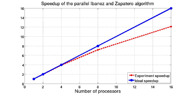
Figure 2: Speedup of the parallel I&Z Algorithm.

3 The Classification and Monte Carlo algorithm

3.1 Introduction

The Monte Carlo approaches for BA option pricing are usually based on continuation value computation [12] or continuation region estimation [8], [10]. The option holder decides either to execute or to continue with the current option contract based on the computed asset value. If the asset value is in the exercise region, he executes the option otherwise he continues to hold the option. Denote that the asset values which belong to the exercise region will form the exercise values and rest will belong to the continuation region. In [8] Picazo et al. propose an algorithm based on the observation that at a given exercise opportunity the option holder makes his decision based on whether the sign of $(exercise\ value-continuation\ value)$ is positive or negative. The author focuses on estimating the continuation region and the exercise region by characterizing the exercise boundary based on these signs. The classification algorithm is used to evaluate such sign values at each opportunity. In this section we briefly describe the sequential algorithm described in [8] and propose a parallel approach followed by performance benchmarks.

3.2 Sequential algorithm

For illustration let us consider a BA option on $d$ underlying assets modeled by Geometric Brownian Motion (GBM). $S_{t}=(S_{t}^{i})$ with $i=1,..,d$. The option price at time $t_{0}$ is defined as follows:

$P_{t_{0}}(S_{t_{0}})=\mathbb{E}\left(\exp{(-r\tau)}\Phi(S_{\tau},\tau)|S_{t_{0}}\right)$

where $\tau$ is the optimal stopping time $\in\{t_{1},..,T\}$, $T$ is the maturity date, $r$ is the constant interest rate and $\Phi(S_{\tau},\tau)$ is the payoff value at time $\tau$. In case of I&Z Algorithm, the optimal stopping time is defined when the underlying asset value crosses the exercise boundary. The CMC algorithm defines the stopping time whenever the underlying asset value makes the sign of $(exercise\ value-continuation\ value)$ positive. Without loss of generality, at a given time $t$ the BA option price on the period $[t,T]$ is given by:

$P_{t}(S_{t})=\mathbb{E}\left(\exp{(-r(\tau-t))}\Phi(S_{\tau},\tau)|S_{t}\right)$

where $\tau$ is the optimal stopping time $\in\{1,..,T\}$. Let us define the difference between the payoff value and the option price at time $t_{m}$ as,

$\beta(t_{m},S_{t_{m}})=\Phi(S_{t_{m}},t_{m})-P_{t_{m}}(S_{t_{m}})$

where $m\in\{1,..,T\}$. The option is exercised when $S_{t_{m}}\in\{x|\beta(t_{m},x)>0\}$ which is the exercise region, and $x$ is the simulated underlying asset value, otherwise the option is continued. The goal of the algorithm is to determinate the function $\beta(\cdot)$ for every opportunity date. However, we do not need to fully parameterize this function. It is enough to find a function $F_{t}(\cdot)$ such that $signF_{t}(\cdot)=sign\beta(t,\cdot)$.

The algorithm consists of two phases. In the first phase, it aims to find a function $F_{t}(\cdot)$ having the same sign as the function $\beta(t,\cdot)$. The AdaBoost or LogitBoost algorithm is used to characterize these functions. In the second phase the option is priced by a standard MC simulation by taking the advantage of the characterization of $F_{t_{m}}(\cdot)$, so for the $(i)^{th}$ MC simulation we get the optimal stopping time $\tau_{(i)}=\min\{t_{m}\in\{t_{1},t_{2},...,T\}|F_{t}(S^{(i)}_{t})>0\}$. The $(i)$ is not the index of the number of assets.

Now, consider a call BA option on the maximum of $d$ underlying assets where the payoff at time $\tau$ is defined as $\Phi(S_{\tau},\tau)=(\max_{i}(S^{i}_{\tau})-K)^{+}$ with $i=1,..,d$. During the first phase of the algorithm, at a given opportunity date $t_{m}$ with $m\in{1,...,N_{T}}$, $N_{1}$ underlying price vectors sized $d$ are simulated. The simulations are performed recursively in backward from $m=T$ to $m=1$. From each price point, another $N_{2}$ paths are simulated from a given opportunity date to the maturity date to compute the “small” BA option price at this opportunity (i.e. $P_{t_{m}}(S_{t_{m}})$). At this step, $N_{1}$ option prices related to the opportunity date are computed. The time step complexity of this step is $\mathbb{O}(N_{1}\times d\times m\times N_{2}\times(N_{T}-m))$. In the classification phase, we use a training set of $N_{1}$ underlying price points and their corresponding option prices at a given opportunity date. In this step, a non–parametric regression is done on $N_{1}$ points to characterize the exercise boundary. This first phase is repeated for each opportunity date. In the second phase, the option value is computed by simulating a large number, $N$, of standard MC simulations with $N_{T}$ exercise opportunities. The complexity of this phase is $\mathbb{O}(d\times N_{T}\times N)$. Thus, the total time steps required for the algorithm can be given by the following formula,

$\mathbb{O}\left(\sum_{m=1}^{N_{T}}N_{1}\times d\times m\times N_{2}\times(N_{T}-m)+N_{T}\times classification(N_{1})+d\times N_{T}\times N\right)$

$\approx\mathbb{O}\left(N_{T}^{2}\times N_{1}\times d\times N_{2}+N_{T}\times(N_{1}+d\times N)\right)$

where $\mathbb{O}(classification(\cdot))$ is the complexity of the classification phase and the details of which can be found in [8]. For the simulations, we use the same option parameters as described in (5), taken from [10], and the parameters for the classification can be found in [8].

$$\begin{array}[]{l}\mbox{$K=100$, {interest rate r = 0.05}, {volatility rate $\sigma$ = 0.2},}\\ \mbox{{dividend $\delta$ = 0.1}, $N_{1}=5e3$, $N_{2}=500$, $N=1e6$, $d=3$ }\\ \mbox{$N_{T}=9$ and $T=3$ years.}\end{array}$$ (9)

Each of the $N_{1}$ points of the training set acts as a seed which is further used to simulate $N_{2}$ simulation paths. From the exercise opportunity $m$ backward to $m-1$, a Brownian motion bridge is used to simulate the price of the underlying asset. The time distribution of each phase of the sequential algorithm for pricing the option (9) is shown in Figure 3. As we can see from the figure, the most computationally intensive part is the data generation phase which is used to compute the option prices required for classification. In the following section we present a parallel approach for this and rest of the phases of the algorithm.

3.3 Parallel approach

The Algorithm 10 illustrates the parallel approach based on CMC Algorithm. At $t_{m}=T$ we generate $N_{1}$ points of the price of the underlying assets, $S_{t_{m}}^{(i)}$, $i=1,..,N_{1}$ then apply the Brownian bridge simulation process to get the price at the backward date, $t_{m-1}$. For simplicity we assume a master–worker programming model for the parallel implementation: the master is responsible for allocating independent tasks to workers and for collecting the results. The master divides $N_{1}$ simulations into $nb$ tasks then distributes them to a number of workers. Thus each worker has $N_{1}/nb$ points to simulate in the [calc] phase. Each worker, further, simulates $N_{2}$ paths for each point from $t_{m}$ to $t_{N_{T}}$ starting at $S_{t_{m}}^{(i)}$ to compute the option price related to the opportunity date. Next the worker calculates the value $y_{j}=(exercise\ value-continuation\ value)$, $j=1,..,N_{1}/nb$. The master collects the $y_{j}$ of these $nb$ tasks from the workers and then classifies them in order to return the characterization model of the associated exercise boundary in the [class] phase.

Algorithm 2 Parallel Classification and Monte Carlo Algorithm

1:  for $t=t_{N_{T}}$ to $t_{1}$ do

2:     for $i=1$ to $N_{1}$ in parallel do

3:        [calc] Computation of training points.

4:     end for

5:     [class] Classification using boosting.

6:  end for

7:  for $i=1$ to $N$ in parallel  do

8:     [mc] The partial option price computation.

9:  end for

10:  Estimation of the final option price by merging the partial prices.

For the classification phase, the master does a non-parametric regression with the set $(x_{(i)},y_{(i)})^{N_{1}}_{i=1}$, where $x_{(i)}=S_{t_{m}}^{(i)}$, to get the function $F_{t_{m}}(x)$ described above in Section (3.2). The algorithm recursively repeats the same procedure for earlier time intervals $[m-1,1]$. As a result we obtain the characterization of the boundaries, $F_{t_{m}}(x)$, at every opportunity $t_{m}$. Using these boundaries, a standard MC simulation, [mc], is used to estimate the option price. The MC simulations are distributed among workers such that each worker has the entire characterization boundary information $(F_{t_{m}}(x),m=1,..,N_{T})$ to compute the partial option price. The master later merges the partially computed prices and estimates the final option price.

3.4 Numerical results and performance

In this section we present the numerical and performance results of the parallel CMC Algorithm. We focus on the standard example of a call option on the maximum of 3 assets as given in (9). As it can be seen, the estimated prices are equivalent to the reference prices presented in Andersen and Broadies [2], which are represented in the “Binomial” column in Table 4. For pricing this option, the sequential execution takes up to 30 minutes and the time distribution for the different phases can be seen in Figure 3. The speed up achieved by the parallel algorithm is presented in Figure 4. We can observe from the figure that the parallel algorithm achieves linear scalability with a fewer number of processors. The different phases of the algorithm scale differently. The MC phase being embarrassingly parallel scales linearly, while, the number of processors has no impact on the scalability of the classification phase. The classification phase is sequential and takes a constant amount of time for the same option. This affects the overall speedup of the algorithm as shown in Figure 4.

$S_{0}$	Price	Variance (95% CI)	Binomial	Error
90	11.295	190.786 (0.027)	11.290	0.005
100	18.706	286.679 (0.033)	18.690	0.016
110	27.604	378.713 (0.038)	27.580	0.024

Table 4: Price of the call BA on the maximum of three assets using CMC Algorithm. ($r=0.05$, $\delta=0.1$, $\sigma=0.2$, $\rho=0.0$, $T=3$, $N=9$ opportunities)

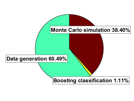
Figure 3: The time distribution for different phases of the sequential Classification–Monte Carlo algorithm. The total time is about 30 minutes.

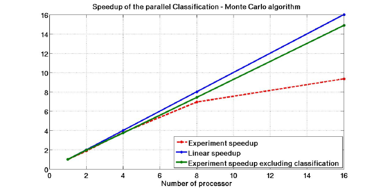
Figure 4: Speedup of the parallel CMC Algorithm.

4 Conclusion

The aim of the study is to develop and implement parallel Monte Carlo based Bermudan/American option pricing algorithms. In this paper, we particularly focused on multi–dimensional options. We evaluated the scalability of the proposed parallel algorithms in a computational grid environment. We also analyzed the performance and the accuracy of both algorithms. While I&Z Algorithm computes the exact exercise boundary, CMC Algorithm estimates the characterization of the boundary. The results obtained clearly indicate that the scalability of I&Z Algorithm is limited by the boundary points computation. The Table 2 showed that there is no effective advantage to increase the number of such points as will, just to take advantage of a greater number of available CPUs. Moreover, the time required for computing individual boundary points varies and the points with slower convergence rate often haul the performance of the algorithm. However, in the case of CMC Algorithm, the sequential classification phase tends to dominate the total parallel computational time. Nevertheless, CMC Algorithm can be used for pricing different option types such as maximum, minimum or geometric average basket options using a generic classification configuration. While the optimal exercise boundary structure in I&Z Algorithm needs to be tailored as per the option type and requires. Parallelizing classification phase presents us several challenges due to its dependency on inherently sequential non–parametric regression. Hence, we direct our future research to investigate efficient parallel algorithms for computing exercise boundary points, in case of I&Z Algorithm, and the classification phase, in case of CMC Algorithm.

5 Acknowledgments

This research is supported by the French “ANR-CIGC GCPMF” project and Grid5000 has been funded by ACI-GRID.

References

- [1] http://perso-math.univ-mlv.fr/users/printems.jacques/.
- [2] L. Andersen and M. Broadie. Primal-Dual Simulation Algorithm for Pricing Multidimensional American Options. Management Science, 50(9):1222–1234, 2004.
- [3] P.P. Boyle, A. Kolkiewicz, and K.S. Tan. Pricing American style options using low discrepancy mesh methods. Forthcoming, Mathematics and Computers in Simulation.
- [4] M. Broadie and J. Detemple. The Valuation of American Options on Multiple Assets. Mathematical Finance, 7(3):241–286, 1997.
- [5] J.C. Cox, S.A. Ross, and M. Rubinstein. Option Pricing: A Simplified Approach. Journal of Financial Economics, 7(3):229–263, 1979.
- [6] P. Glasserman. Monte Carlo Methods in Financial Engineering. Springer, 2004.
- [7] S. Haber. Parameters for Integrating Periodic Functions of Several Variables. Mathematics of Computation, 41(163):115–129, 1983.
- [8] F.J. Hickernell, H. Niederreiter, and K. Fang. Monte Carlo and Quasi-Monte Carlo Methods 2000: Proceedings of a Conference Held at Hong Kong Baptist University, Hong Kong SAR, China. Springer, 2002.
- [9] K. Huang and R.K. Thulasiram. Parallel Algorithm for Pricing American Asian Options with Multi-Dimensional Assets. Proceedings of the 19th International Symposium on High Performance Computing Systems and Applications, pages 177–185, 2005.
- [10] A. Ibanez and F. Zapatero. Monte Carlo Valuation of American Options through Computation of the Optimal Exercise Frontier. Journal of Financial and Quantitative Analysis, 39(2):239–273, 2004.
- [11] P. L’Ecuyer, L. Meliani, and J. Vaucher. SSJ: SSJ: a framework for stochastic simulation in Java. Proceedings of the 34th conference on Winter simulation: exploring new frontiers, pages 234–242, 2002.
- [12] F.A. Longstaff and E.S. Schwartz. Valuing American options by simulation: a simple least-squares approach. Review of Financial Studies, 2001.
- [13] G. Pagès and J. Printems. Optimal quadratic quantization for numerics: the Gaussian case. Monte Carlo Methods and Applications, 9(2):135–165, 2003.
- [14] I.H. Sloan and S. Joe. Lattice Methods for Multiple Integration. Oxford University Press, 1994.
- [15] R.K. Thulasiram and D.A. Bondarenko. Performance Evaluation of Parallel Algorithms for Pricing Multidimensional Financial Derivatives. The International Conference on Parallel Processing Workshops (ICPPW 02), 1530, 2002.
- [16] I.M. Toke. Monte Carlo Valuation of Multidimensional American Options Through Grid Computing. Lecture notes in computer science, Springer-Verlag, Volume 3743:page 462, 2006.