Coupled Dynamics on Networks

Abstract

We study the synchronization of coupled dynamical systems on a variety of networks. The dynamics is governed by a local nonlinear map or flow for each node of the network and couplings connecting different nodes via the links of the network. For small coupling strengths nodes show turbulent behavior but form synchronized clusters as coupling increases. When nodes show synchronized behaviour, we observe two interesting phenomena. First, there are some nodes of the floating type that show intermittent behaviour between getting attached to some clusters and evolving independently. Secondly, we identify two different ways of cluster formation, namely self-organized clusters which have mostly intra-cluster couplings and driven clusters which have mostly inter-cluster couplings.

1 Introduction

Several complex systems have underlying structures that are described by networks or graphs [1, 2]. Recent interest in networks is due to the discovery that several naturally occurring networks come under some universal classes and they can be simulated with simple mathematical models, viz small-world networks [3], scale-free networks [4] etc.

Several networks in the real world consist of dynamical elements interacting with each other and the interactions define the links of the network. Several of these networks have a large number of degrees of freedom and it is important to understand their dynamical behavior. Here, we study the synchronization and cluster formation in networks consisting of interacting dynamical elements. A general model of coupled dynamical systems on networks will consist of the following three elements.

1. The evolution of uncoupled elements.

2. The nature of couplings.

3. The topology of the network.

Most of the earlier studies of synchronized cluster formation in coupled chaotic systems have focused on networks with large number of connections ($\sim N^{2}$) [6]. In this paper, we consider networks with number of connections of the order of $N$. This small number of connections allows us to study the role that different connections play in synchronizing different nodes and the mechanism of synchronized cluster formation. The study reveals two interesting phenomena. First, when nodes form synchronized clusters, there can be some nodes which show an intermittent behaviour between independent evolution and evolution synchronized with some cluster. Secondly, the cluster formation can be in two different ways, driven and self-organized phase synchronization [5]. The connections or couplings in the self-organized phase synchronized clusters are mostly of the intra-cluster type while those in the driven phase synchronized clusters are mostly of the inter-cluster type.

2 Coupled dynamical systems and synchronized clusters

Consider a network of $N$ nodes and $N_{c}$ connections (or couplings) between the nodes. Let each node of the network be assigned an $m$-dimensional dynamical variable ${\bf x}^{i},i=1,2,\ldots,N$. A very general dynamical evolution can be written as

$$\frac{d{\bf x}_{i}}{dt}={\bf F}(\{{\bf x}_{i}\}).$$ (1)

In this paper, we consider a separable case and the evolution equation can be written as,

$$\frac{d{\bf x}_{i}}{dt}={\bf f}({\bf x}_{i})+\frac{\epsilon}{k_{i}}\sum_{j\in\{k_{i}\}}{\bf g}({\bf x}_{j}).$$ (2)

where $\epsilon$ is the coupling constant, $k_{i}$ is the degree of node $i$, and $\{k_{i}\}$ is the set of nodes connected to the node $i$. A sort of diffusion version of the evolution equation (2) is

$$\frac{d{\bf x}_{i}}{dt}={\bf f}({\bf x}_{i})+\frac{\epsilon}{k_{i}}\sum_{j\in\{k_{i}\}}\left({\bf g}({\bf x}_{j})-{\bf g}({\bf x}_{i})\right).$$ (3)

Discrete versions of Eqs. (2) and (3) are

$${\bf x}_{i}(t+1)={\bf f}({\bf x}_{i}(t))+\frac{\epsilon}{k_{i}}\sum_{j\in\{k_{i}\}}{\bf g}({\bf x}_{j}(t)).$$ (4)

and

$${\bf x}_{i}(t+1)={\bf f}({\bf x}_{i}(t))+\frac{\epsilon}{k_{i}}\sum_{j\in\{k_{i}\}}\left({\bf g}({\bf x}_{j}(t))-{\bf g}({\bf x}_{i}(t))\right).$$ (5)

For the discrete evolution we use logistic or circle maps while for the continuous case we use Lorenz or Rössler systems.

2.1 Phase synchronization and synchronized clusters

Synchronization of coupled dynamical systems [7] is manifested by the appearance of some relation between the functionals of different dynamical variables. The exact synchronization corresponds to the situation where the dynamical variables for different nodes have identical values. The phase synchronization corresponds to the situation where the dynamical variables for different nodes have some definite relation between their phases [8, 9]. When the number of connections in the network is small ($N_{C}\sim N$) and when the local dynamics of the nodes (i.e. function $f(x)$) is in the chaotic zone, and we look at exact synchronization, we find that only few synchronized clusters with small number of nodes are formed. However, when we look at phase synchronization, synchronized clusters with larger number of nodes are obtained. Hence, in our numerical study we concentrate on phase synchronization.

3 General properties of synchronized dynamics

We consider some general properties of synchronized dynamics. They are valid for any coupled discrete and continuous dynamical systems. Also, these properties are applicable for exact as well as phase or any other type of synchronization and are independent of the type of network.

3.1 Behavior of individual nodes

As the network evolves, it splits into several synchronized clusters. Depending on their asymptotic dynamical behaviour the nodes of the network can be divided into three types.
(a) Cluster nodes: A node of this type synchronizes with other nodes and forms a synchronized cluster. Once this node enters a synchronized cluster it remains in that cluster afterwards.
(b) Isolated nodes: A node of this type does not synchronize with any other node and remains isolated for all the time.
(c) Floating Nodes: A node of this type keeps on switching intermittently between an independent evolution and a synchronized evolution attached to some cluster.

Of particular interest are the floating nodes and we will discuss some of their properties afterwards.

3.2 Mechanism of cluster formation

The study of the relation between the synchronized clusters and the couplings between the nodes represented by the adjacency matrix $C$ shows two different mechanisms of cluster formation [5, 10].
(i) Self-organized clusters: The nodes of a cluster can be synchronized because of intra-cluster couplings. We refer to this as the self-organized synchronization and the corresponding synchronized clusters as self-organized clusters.
(ii) Driven clusters: The nodes of a cluster can be synchronized because of inter-cluster couplings. Here the nodes of one cluster are driven by those of the others. We refer to this as the driven synchronization and the corresponding clusters as driven clusters.

In our numerical studies we have been able to identify ideal clusters of both the types, as well as clusters of the mixed type where both ways of synchronization contribute to cluster formation. (Fig. 1 of Ref. [5] gives examples of ideal as well as mixed clusters in coupled map networks.) In general we find that the scale free networks and the Caley tree networks lead to better cluster formation than the other types of networks with the same average connectivity.

Geometrically the two mechanisms of cluster formation can be easily understood by considering a tree type network. A tree can be broken into different clusters in different ways.
(a) A tree can be broken into two or more disjoint clusters with only intra-cluster couplings by breaking one or more connections. Clearly, this splitting is not unique and will lead to self-organized clusters. Figure 1(a) shows a tree forming two synchronized clusters of self-organized type. This situation is similar to an Ising ferromagnet where domains of up and down spins can be formed.
(b) A tree can also be divided into two clusters by putting connected nodes into different clusters. This division is unique and leads to two clusters with only inter-cluster couplings, i.e. driven clusters. Figure 1(b) shows a tree forming two synchronized clusters of the driven type. This situation is similar to an Ising anti-ferromagnet where two sub-lattices of up and down spins are formed.
(c) Several other ways of splitting a tree are possible. E.g. it is easy to see that a tree can be broken into three clusters of the driven type. This is shown in figure 1(c). There is no simple magnetic analog for this type of cluster formation. It can be observed close to a period three orbit. We note that four or more clusters of the driven type are also possible. As compared to the cases (a) and (b) discussed above which are commonly observed, the clusters of case (c) are not so common and are observed only for some values of the parameters.

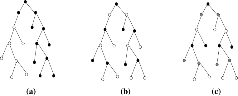
Figure 1: Different ways of cluster formation in a tree structure are demonstrated. The open, solid and gray circles show nodes belonging to different clusters. (a) shows two clusters of the self-organized type, (b) shows two clusters of driven type and (c) shows three clusters of the driven type.

4 Linear stability analysis

A suitable network to study the stability of self-organized synchronized clusters is the globally coupled network. The stability of globally coupled maps is well studied in the literature [11, 12, 13]. An ideal example to consider the stability of the driven synchronized state is a complete bipartite network. A complete bipartite network consists of two sets of nodes with each node of one set connected with all the nodes of the other set and no connection between the nodes of the same set. Let $N_{1}$ and $N_{2}$ be the number of nodes belonging to the two sets. We define a bipartite synchronized state as the one that has all $N_{1}$ elements of the first set synchronized to some value, say ${\bf X}_{1}(t)$, and all $N_{2}$ elements of the second set synchronized to some other value, say ${\bf X}_{2}(t)$.

All the eigenvectors and the eigenvalues of the Jacobian matrix for the bipartite synchronized state can be determined explicitly. The eigenvectors of the type $(\alpha,\ldots,\alpha,\beta,\ldots,\beta)^{T}$ determine the synchronization manifold and this manifold has dimension two. All other eigenvectors correspond to the transverse manifold. Lyapunov exponents corresponding to the transverse eigenvectors for Eq. (5) with one dimensional variables and $g(x)=f(x)$ are

$$\lambda_{1} = \ln|(1-\epsilon)|+\frac{1}{\tau}\lim_{\tau\to\infty}\sum^{\tau}_{t=1}\ln|f^{\prime}(X_{1})|,$$

$$\lambda_{2} = \ln|(1-\epsilon)|+\frac{1}{\tau}\lim_{\tau\to\infty}\sum^{\tau}_{t=1}\ln|f^{\prime}(X_{2})|,$$ (6)

and $\lambda_{1}$ and $\lambda_{2}$ are respectively $N_{1}-1$ and $N_{2}-1$ fold degenerate [10]. Here, $f^{\prime}_{(}X_{1})$ and $f^{\prime}_{(}X_{2})$ are the derivatives of $f(x)$ at $X_{1}$ and $X_{2}$ respectively. The synchronized state is stable provided the transverse Lyapunov exponents are negative. If $f^{\prime}$ is bounded then from Eqs. (6) we see that for $\epsilon$ larger than some critical value, $\epsilon_{b}(<1)$, bipartite synchronized state will be stable. Note that this bipartite synchronized state will be stable even if one or both the remaining Lyapunov exponents corresponding to the synchronization manifold are positive, i.e. the trajectories are chaotic. The linear stability analysis for other type of couplings and dynamical systems can be done along similar lines.

5 Floating nodes

We had noted earlier that the nodes can be divided into three types, namely cluster nodes, isolated nodes and floating nodes, depending on the asymptotic behavior of the nodes. Here, we discuss some properties of the floating nodes which show an intermittent behavior between synchronized evolution with some cluster and an independent evolution.

Let $\tau$ denote the residence time of a floating node in a cluster (i.e. the continuous time interval that the node is in a cluster). Figure 2 plots the frequency of residence time $\nu(\tau)$ of a floating node as a function of the residence time $\tau$. A good straight line fit on log-linear plot shows an exponential dependence,

$$\nu(\tau)\sim\exp(-\tau/\tau_{r})$$ (7)

where $\tau_{r}$ is the typical residence time for a given node. We have also studied the distribution of the time intervals for which a floating node is not synchronized with a given cluster. This also shows an exponential distribution.

Figure 2: The figure plots the frequency of residence time $\nu(\tau)$ of a floating node in a cluster as a function of the residence time $\tau$. A good straight line fit on log-linear plot shows exponential dependence.

Let us now consider the condition for the occurrence of floating nodes. Consider a floating node in a cluster. The stability of this cluster is ensured if the transverse Lyapunov exponents are all negative. The floating node will leave the cluster provided the conditional Lyapunov exponent for this node, assuming that the other nodes in the cluster remain synchronized, changes sign and becomes positive. Thus the fluctuation of the conditional Lyapunov exponent about zero can be taken as the condition for the existence of a floating node.

Several natural systems show examples of floating nodes, e.g. some birds may show intermittent behaviour between free flying and flying in a flock. An interesting example in physics is that of particles or molecules in a liquid in equilibrium with its vapor where the particles intermittently belong to the liquid and vapor. Under suitable conditions it is possible to argue that the residence time of a tagged particle in the liquid phase should have an exponential distribution [10], i.e. a behavior similar to that of the floating nodes (Eq. (7)).

6 Conclusion and Discussion

We have studied the properties of coupled dynamical elements on different types of networks. We find that in the course of time evolution they form synchronized clusters.

In several cases when synchronized clusters are formed there are some isolated nodes which do not belong to any cluster. More interestingly there are some floating nodes which show an intermittent behavior between an independent evolution and an evolution synchronized with some cluster. The residence time spent by a floating node in the synchronized cluster shows an exponential distribution.

We have identified two mechanisms of cluster formation, self-organized and driven phase synchronization. For self-organized clusters intra-cluster couplings dominate while for driven clusters inter-cluster couplings dominate.

References

- [1] S. H. Strogatz, Nature 410 (2001) 268 and references theirin.
- [2] R. Albert and A. L. Barabäsi, Rev. Mod. Phys. 74 (2002) 47 and references theirin.
- [3] D. J. Watts and S. H. Strogatz, Nature (London) 393 (1998) 440.
- [4] A. -L. Barabäsi, R. Albert, Science 286 (1999) 509.
- [5] S. Jalan, R. E. Amritkar, Phys. Rev. Lett. 90 (2003) 014101.
- [6] K. Kaneko, Physica D124 (1998) 322.
- [7] A. Pikovsky, M. Rosenblum and J. Kurth, Synchronization : A universal concept in nonlinear dynamics, Cambridge University Press, 2001.
- [8] M. G. Rosenblum, A. S. Pikovsky, and J. Kurth, Phys. Rev. Lett. 76, (1996) 1804; W. Wang, Z. Liu, Bambi Hu, Phys. rev. Lett. 84 (2000) 2610.
- [9] S. C. Manrubia and A. S. Mikhailov, Europhys. Lett. 53 (4) (2001) 451.
- [10] S. Jalan, R. E. Amritkar and C. K. Hu, unpublished.
- [11] H. Fujisaka and T. Yamada, Prog. Theo. Phys. 69, 32 (1983).
- [12] P. M. Gade, Phys. Rev. E54 (1996) 64.
- [13] M. Ding and W. Yang, Phys Rev E56 (1997) 4009.