Stellar Rotation in Field and Cluster B-Stars

Abstract

We present the results of a spectroscopic investigation of 108 nearby field B-stars. We derive their key stellar parameters, $V\sin i$, $T_{\rm eff}$, $\log g$, and $\log g_{\rm polar}$, using the same methods that we used in our previous cluster B-star survey. By comparing the results of the field and the cluster samples, we find that the main reason for the overall slower rotation of the field sample is that it contains a larger fraction of older stars than found in the (mainly young) cluster sample.

1 Introduction

It is a curious but well known fact that field B-stars rotate slower than cluster B-stars (Abt, Levato, & Grosso, 2002; Strom, Wolff, & Dror, 2005; Huang & Gies, 2006a; Wolff et al., 2007), but the explanation for the difference is still controversial. One possible solution is that field B-stars represent a population that contains more evolved stars than cluster B-stars do. They appear to rotate slower because stars generally spin down as they evolve (Abt et al., 2002; Huang & Gies, 2006a, b). On the other hand, Strom et al. (2005) and Wolff et al. (2007) suggest that difference in rotation rates between field and cluster B-stars is mainly due to the difference between the initial conditions of the stellar forming regions. The denser the environment (such as in young open clusters), the more rapid rotators can form. The second explanation brings more attention to the possible connection between stellar rotation and the physical mechanisms playing a role during the star formation stage. A plausible higher accretion rate around a forming star in a denser region may lead to a higher initial angular momentum and a shorter accretion disk lifetime with its associated spin-down effects via magnetic interactions between the star and the disk.

Because both the evolutionary status of stars and the initial conditions of their forming regions may influence their rotation rates, knowing the evolutionary status of these stars precisely becomes a prerequisite for the solution of this puzzle. With this in mind, we made a spectroscopic investigation of 108 field B-stars using the same methods that we applied in our previous cluster B-star survey (Huang & Gies, 2006a, b). There are two advantages over previous studies of this topic: 1) Because we apply identical spectroscopic methods to both the field and cluster samples, the influence of any imperfection in our methods on the final comparisons will be reduced to a minimum; 2) We use the estimated $\log g_{\rm polar}$ as an indicator of stellar evolutionary status, which is more accurate and reliable for large numbers of stars with diverse masses and rotation rates. We describe our derivation of the key stellar parameters of a field sample of B-stars in next section. The results of a comparison between the field sample and the cluster sample are reported in Section 3, and a short discussion and our conclusion are given in Section 4.

2 Field B-Star Sample

Our field B-star sample was selected from the NOAO Indo-U.S. Library of Coudé Feed Stellar Spectra (Valdes et al., 2004). This library contains moderate resolution spectra (FWHM = $1-2$Å) of 1273 stars that were obtained with the 0.9-m Coudé Feed telescope at Kitt Peak National Observatory. Roughly about 140 B-star spectra are found in this library. These spectra are comparable in S/N and resolution to those analyzed in our previous cluster B-star survey.

Following the exact same procedure that we applied to cluster B-stars (Huang & Gies, 2006a, b), we obtained the stellar parameters of 108 B stars in our final sample: the projected rotational velocity $V\sin i$, the effective temperature $T_{\rm eff}$, the apparent gravity $\log g$, and the estimated polar gravity $\log g_{\rm polar}$. These results are summarized in Table 1. We excluded all double-lined spectroscopic binaries (SB2) from the sample because the derived parameters of these objects are not reliable. The errors are estimated from the deviations between the observed and model profiles (see Huang & Gies 2006b), and inclusion of uncertainties related to the continuum placement may increase these errors by $\approx 40\%$.

The $V\sin i$ values were derived by fitting synthetic model profiles of He I $\lambda 4471$ (or Mg II $\lambda 4481$ if the He I line is too weak) to the observed profiles, using realistic physical models of rotating stars (including Roche geometry and gravity darkening). The details of this step are described in Huang & Gies (2006a). One concern about the derived $V\sin i$ values is that we do not know the exact instrumental broadening data of the NOAO Indo-U.S. Library spectra for the investigated region (4470 - 4480 Å), and assumed only the lower limit of the given FWHM range, 1 Å, in the convolution of our synthesized line profiles. An underestimation of the instrumental broadening can lead to higher derived $V\sin i$ values. In order to determine and then correct the possible systematic errors caused by the uncertainty in the assumed instrumental broadening, we also obtained high resolution spectra ($R=\lambda/\triangle\lambda\sim 42000$) of 34 stars in our sample from the ELODIE archive (Moultaka et al., 2004). By comparing the $V\sin i$ values derived from the NOAO library to those from the ELODIE library, we found the best relationship between them can be written as

$$V\sin i_{\rm Elodie}\simeq\sqrt{(V\sin i_{\rm NOAO})^{2}-(46~{}{\rm km~{}s}^{-1})^{2}}.$$ (1)

For the stars in our sample that are not found in the Elodie library, we corrected their $V\sin i$ using eq. 1 for $V\sin i_{\rm NOAO}>46$ km s^-1, and we set $V\sin i=0$ for $V\sin i_{\rm NOAO}\leq 46$ km s^-1. The corrected $V\sin i$ and its numerical fitting error are given in columns (6) and (7) of Table 1. A comparison of the derived $V\sin i$ values between our results and those from Abt et al. (2002) is illustrated in Figure 1. The good agreement in the low $V\sin i$ region indicates that our corrections to $V\sin i$ are properly assigned. In the high $V\sin i$ region, our results are systematically greater than the results from Abt et al. (2002). This discrepancy is not surprising, considering that our models take the gravity darkening effect into account. Townsend, Owocki, & Howarth (2004) showed that the $V\sin i$ derived from fitting the He I $\lambda 4471$ line could be lower by as much as 10-20% for a rapid rotator if the strong gravity darkening effect on its surface is ignored. The most discrepant point in Figure 1 is the star HD 172958. Our $V\sin i$ measurement of this star (167 km s^-1) is similar to the measurements by Peacock & Connon-Smith (1987) and Wolff & Preston (1978) (175 km s^-1). The much larger value measured by Abt et al. (2002), $V\sin i=315$ km s^-1, might result if the star is an unresolved, doubled-line binary that was observed at a time of larger relative Doppler shifts, but the star is not a known binary.

The effective temperature and gravity were derived by fitting the H$\gamma$ profile (see details in Huang & Gies 2006b). The results and the associated numerical fitting errors are listed in columns (2) to (5) of Table 1. As pointed out by Huang & Gies (2006b), the derived $\log g$ values represent an average of gravity over the visible hemisphere of these rotating stars. They may not be good indicators of stellar evolutionary status, especially for rapid rotators that have much lower gravity in the equatorial area caused by the strong centrifugal force. Following the method described in Huang & Gies (2006b), we made a statistical correction to estimate the polar gravity of each star from its derived $V\sin i$, $T_{\rm eff}$, and $\log g$, and the resulting polar gravity is listed in column (8) of Table 1. Our estimates of $\log g_{\rm polar}$ are consistent with the available observations. For example, one of our targets is Regulus (HD 87901) that was recently resolved by the CHARA Array optical long baseline interferometer (McAlister et al., 2005). Models of the spectroscopy and interferometry of this rotationally deformed star lead directly to a polar gravity of $\log g_{\rm polar}=3.98$, which compares well with the statistical estimate here of $\log g_{\rm polar}=3.95$. Furthermore, we used our derived $\log g_{\rm polar}$ values with masses estimated from Figure 3 to derive radii, luminosities, bolometric corrections, and absolute magnitudes. We combined these with the observed magnitudes to find distance estimates, and a comparison of the derived distances with those from Hipparcos (van Leeuwen, 2007) shows good consistency. We note for completeness that in a sample of ten stars in common, Fitzpatrick & Massa (2005) find temperatures that are $\approx 4\%$ larger and gravities that are $\approx 0.1$ dex greater than our values. While these differences between results from spectral flux and H$\gamma$ fitting are interesting, they are insignificant for our purpose of comparing the parameters of the field and cluster B-stars in a consistent manner.

3 A Comparison of Field and Cluster B Stars

The recent studies (Abt et al., 2002; Strom et al., 2005; Huang & Gies, 2006a; Wolff et al., 2007) that found that field B-stars appear to rotate slower than cluster B-stars were mainly based on the field sample from Abt et al. (2002) that includes roughly 1100 bright field B-stars selected from the Bright Star Catalogue (Hoffleit & Jaschek, 1982). We note that both this and our own smaller sample of B-stars are not volume-limited but tend to select from the intrinsically brighter members of the population. Furthermore, both samples include some members of nearby OB associations and moving groups, which are not strictly “field” objects. Nevertheless, these field samples are similar enough in their sampling of the spectral types, luminosities, and true field star content that we can use both to compare with the cluster star rotational properties. The Abt et al. field sample (ALG02) contains a total of 902 B-stars of classes III-V, excluding all SB2s, which we use in our statistical analysis below. Our field sample consists of only 108 B-stars, so one might question whether its content and size are sufficient to represent a field star population similar to that of ALG02. The spectral sub-type distribution of our field sample and of the ALG02 sample are very similar (see Table 2). Furthermore, we show in Figure 2 that the cumulative distribution functions of projected rotational velocities $V\sin i$ appear to be the same. The mean $V\sin i$ of our field sample is $114\pm 9$ km s^-1 while the mean $V\sin i$ of the ALG02 sample is $116\pm 3$ km s^-1. A Kolmogorov-Smirnov (KS) test shows that these two samples have a probability of 0.72 to be drawn from the same parent sample. Thus, we conclude that our limited sample makes a fair representation of the larger field sample of ALG02 and of the rotational properties associated with this group of stars.

The cluster B-star sample used for comparison is extracted from our previous survey of B-stars in 19 open clusters (Huang & Gies, 2006a, b). After removing all O-stars and SB2s, 432 cluster B-stars remain in this sample, which covers a range of age from 6 to 72 Myr (the average is 12.5 Myr). The mean $V\sin i$ of the cluster sample is $146\pm 4$ km s^-1, which is definitely higher than the corresponding value of the field sample. The cumulative curve for the cluster sample is also significantly different from that of the field sample (Fig. 2). The KS probability that our field and cluster samples are drawn from the same parent sample is as low as 0.001.

The distributions of the field and the cluster B-star samples in the $\log T_{\rm eff}-\log g_{\rm polar}$ plane are plotted in Figure 3. We see that along each evolutionary track the field stars are more evenly distributed in $\log g_{\rm polar}$ than is the case for the cluster stars, which mainly have higher $\log g_{\rm polar}$ (near the ZAMS). This indicates that the field B-star sample contains a larger fraction of older stars (i.e., with lower $\log g_{\rm polar}$) than found in the cluster B-star sample. If the stars in the field sample spin down with time in a similar way as those in the cluster sample (Huang & Gies, 2006b), then it is not surprising that the field sample with more older B-stars appears to be rotating slower than the cluster sample. Note that the cluster sample contains relatively more massive stars compared to the field star sample because the cluster targets were typically selected from the brighter, more massive cluster members.

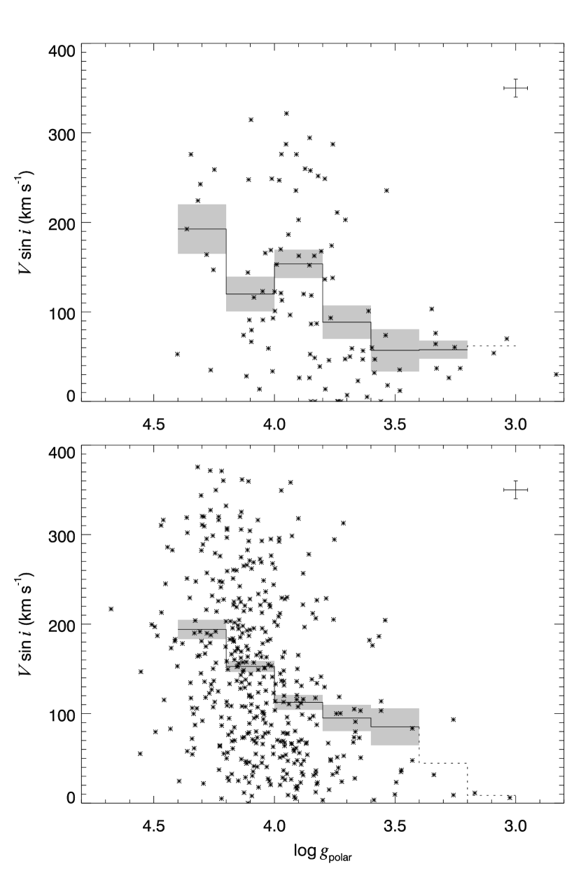
Figure 4: The distribution of the field (top) and cluster (bottom) sample B-stars in the $\log g_{\rm polar}-V\sin i$ plane. The average errors in $\log g_{\rm polar}$ and $V\sin i$ are plotted in the top right corner of each panel. The solid line shows the mean $V\sin i$ of each 0.2 dex bin of $\log g_{\rm polar}$ that contains six or more measurements while the dotted line shows the same for the rest of bins. The shaded areas indicate the associated error of the mean in each bin.

Is the larger fraction of older B-stars in the field sample the dominant cause of its apparent slow rotation or do some additional factors, such as the initial conditions and environment, need to be considered? In order to investigate this, we plot in Figure 4 the $V\sin i$ distributions of both the field and cluster samples against $\log g_{\rm polar}$. Figure 4 also illustrates the mean $V\sin i$ of stars in each bin of 0.2 dex in $\log g_{\rm polar}$ (solid line) and the associated standard deviation of the mean (shaded area). The advantage of using Figure 4 is that the evolutionary spin down effect is dramatically revealed as we compare the stellar rotation of the two samples in each $\log g_{\rm polar}$ bin. The overall decrease in mean $V\sin i$ with lower $\log g_{\rm polar}$ shows clearly that the spin down process exists in both samples. By comparing the mean $V\sin i$ of corresponding bins, we found that it is difficult to draw a firm conclusion about which sample rotates faster. At each evolutionary stage (indicated by $\log g_{\rm polar}$), the B-stars in these two samples appear to rotate equally fast. Thus, the overall slowness of rotation in the field sample is mainly due to the larger percentage of its content occupying the bins of lower $\log g_{\rm polar}$.

Note that we are interpreting the line broadening solely in terms of rotation, but Ryans et al. (2002) and Dufton et al. (2006) find that macroturbulent broadening is also important among the luminous supergiants (where it may amount to velocities of 20 – 60 km s^-1). We have only seven stars in the sample with $\log g_{\rm polar}<3.0$, and these have measured $V\sin i$ velocities of 31 – 59 km s^-1, i.e., comparable to the expected macroturbulent velocities. Thus, we regard the $V\sin i$ values of the stars with low $\log g_{\rm polar}$ as upper limits, and the trend of declining rotation velocity with lower $\log g_{\rm polar}$ may actually be steeper than indicated in the low $\log g_{\rm polar}$ part of Figure 4.

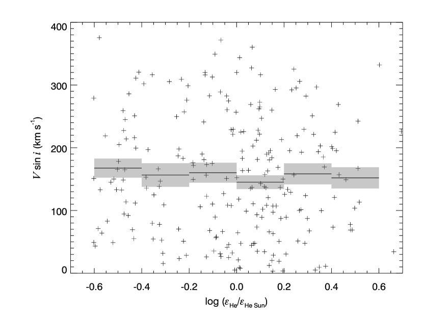
Figure 5: The distribution of the late B-stars ($T_{\rm eff}<20000$ K) in our cluster sample in the $\log(\epsilon_{\rm He}/\epsilon_{\rm He\odot})-V\sin i$ plane. The thick lines indicate the mean $V\sin i$ value of each 0.2 dex bin of $\log(\epsilon_{\rm He}/\epsilon_{\rm He\odot})$. The shadowed areas show the error of the mean in each bin.

One possible concern about the comparison made above is that many late B-stars in our cluster sample are found to have non-solar helium abundances (Huang & Gies, 2006b). Since the hydrogen abundance will be lower in helium enriched atmospheres, the change in atmospheric opacity may cause a change in the appearance of the H$\gamma$ profile that could lead to erroneous derived values of $T_{\rm eff}$ and $\log g$. We checked this possibility by measuring the H$\gamma$ profile in synthetic model spectra for He-peculiar stars calculated by C. S. Jeffrey using the Sterne/Spectrum LTE codes (Jeffrey, Woolf, & Pollacco, 2001). Our results are shown in Table 3 that lists the fraction of H and He atoms by number and our derived $T_{\rm eff}$ and $\log g$ for three temperature cases. The three rows in the table give the results for sub-solar He, solar He, and enhanced He, respectively. Ideally, we should recover exactly the assumed model $T_{\rm eff}$ and $\log g$ for the solar He case, but our scheme arrives at temperatures that are somewhat low (especially at higher $T_{\rm eff}$; for the expected values of 16000K/4.0, we obtain derived values of 15200K/3.95). We suspect that this systematic difference reflects differences between the LTE codes Sterne/Spectrum and the LTE codes ATLAS9/SYNSPEC that we used to develop the H$\gamma$ calibration. While these differences are significant, they are not important for our analysis here where we are making a differential comparison between the cluster and field samples using the same method to obtain the stellar parameters. What is important are the relative changes as the He abundance increases. We see that He enrichment results in a deeper H$\gamma$ profile that is interpreted in our scheme mainly as a decrease in the resulting temperature while changes in the derived gravity are small. Furthermore, we show in Figure 5 that we find no evidence of a correlation between He abundance and $V\sin i$ among the late B stars ($T_{\rm eff}<20000K$) in our cluster sample. Thus, any corrections to the gravity that might be applied to the He-peculiar star subset would be too small to change the rotational trends seen in Figure 4.

4 Discussion and Conclusions

Our findings in previous section seem to support the first explanation mentioned in §1, i.e., field B-stars rotate slower statistically because they represent an older population than cluster B-stars. The projected rotational velocities with each $\log g_{\rm polar}$ bin (corresponding to evolutionary state) appear to be very similar in the field and cluster samples, which suggests that any differences in environmental factors at birth between the field and cluster samples has little influence on their present rotational properties. This conclusion differs from that of Strom et al. (2005) and Wolff et al. (2007) who argue that the stellar number density at formation affects the rotational velocity distribution.

Our field sample contains 108 B-stars. The relatively small sample size precludes an analysis of subsets based on binned mass ranges. This raises a question: can we use the whole field sample of B-stars, which span a large range of mass and main sequence (MS) lifetime, to compare with the cluster sample, and still draw meaningful conclusions? The answer is yes, since our method of comparison is based on the estimated polar gravity $\log g_{\rm polar}$ of individual B-stars. For all subtypes of MS B-stars, the surface $\log g$ falls in a range between 4.2 – 4.3 (for the zero-age main sequence, ZAMS) to 3.4 – 3.6 (for the terminal-age main sequence, TAMS), as shown in Figure 3. The evolutionary spin down of a MS B-star is mainly due to the evolutionary increase of its moment of inertia (and stellar radius) and/or stellar wind mass loss. However, compared to the more massive O-stars, the stellar winds of MS B-stars are generally weak, so wind mass loss plays a minor role in spin down. Thus, the evolutionary changes in stellar properties, such as stellar radius and moment of inertia, will be the major cause of evolutionary spin down. These properties are directly related to surface $\log g$ of the star (or more accurately, $\log g_{\rm polar}$ for a rotating star). In this sense, consideration of B-stars binned in groups of similar $\log g_{\rm polar}$ is a reasonable means to search for evidence of changes in the mean rotational properties with advancing evolutionary state.

Strom et al. (2005) relied on the Strömgren $\beta$ and $c_{0}$ indices to select their objects in both the field and cluster samples. We note, however, that estimates of surface gravity derived from fitting the H$\gamma$ line profile are generally more reliable than those based upon $\beta$ index, which has a larger intrinsic error (since $\beta$ measures the difference in magnitude between a narrow band and a wide band centered at H$\beta$). Thus, even though the cluster and field samples were selected from the same area in the $\beta-c_{0}$ plane, they may still contain populations in different evolutionary states (i.e., over a greater range in gravity). The cluster sample from Strom et al. (2005) is known to be young because it consists of member stars from young open clusters (h and $\chi$ Persei) while the field sample may include a lot of older stars because its content relies on the $\beta-c_{0}$ selection criterion. Smalley & Dworetsky (1995) calculated a grid of synthetic $\beta$ indices applicable to B-stars (given in Table 7 of their paper). The differences in $\beta$ index between ZAMS ($\log g=4.0$) and TAMS ($\log g=3.5$) B-stars are only about 0.04 – 0.05 mag. Since the Strömgren data collected by Strom et al. (2005) for the field B-stars came from diverse sources and have errors of 0.01 - 0.02 mag, it is not easy to distinguish between the evolved and unevolved stars based upon the $\beta$ index alone. Thus, despite their best efforts to compare the rotational velocities of comparably evolved stars in $h$ and $\chi$ Per and the field, Strom et al. (2005) probably included a significant fraction of more evolved stars in the field sample. Our field sample has 21 stars in common with the low mass group (group 1) of the field sample from Strom et al. (2005), the group with the largest difference in the $V\sin i$ cumulative distribution from their cluster sample. Among these 21 stars, 14 have $\log g_{\rm polar}<4.0$. Figure 3 shows that the majority of cluster B-stars with mass less than 5 $M_{\odot}$ has $\log g_{\rm polar}>4.0$. If we assume that the rest of field B-stars in their group 1 are similar to these 21 stars, the slower rotation in group 1 of their field sample can be naturally explained by its older population, instead of the initial conditions (a low density environment of the star forming region) as suggested in their paper.

Wolff et al. (2007) investigated stellar samples from both low density and high density stellar environments. In their analysis, they first inspected the evolutionary effect (spin-down) on stellar rotation, and concluded that the evolutionary effect is too small to account for the difference in stellar rotation that exists between the low and high density samples. However, the evolutionary status of individual stars in their samples is based on the estimated age of the parent association or cluster only. This approach to evolutionary change is less specific than our estimate based upon the polar gravity of each star, since the individual cluster samples may contain quite different proportions of evolved to unevolved stars. Thus, it is possible that the samples considered by Wolff et al. (2007) contain stars that occupy a wider range of evolutionary state than assumed. Consequently, their comparison between the low-density and high-density cumulative probability curves that are based on the whole sample may be influenced more by the evolutionary effect on stellar rotation than the authors realized.

In summary, our spectroscopic investigation of the stellar rotation of 108 field B-stars suggests that the field B-stars contain a larger fraction of more evolved stars than found among our sample of young cluster stars (with an average age of 12.5 Myr) and that makes the field stars appear to rotate slower as whole. This is not a surprising result, since most of the bright field stars belong to the local Gould’s Belt structure that has an expansion age of 30 to 60 Myr (Torra, Fernández & Figueras, 2000). At this point, we do not see any significant differences between the rotational distributions of the field and young cluster B-stars when considered as a function of evolutionary state. We applied identical spectroscopic methods to both the field and cluster samples, and this should minimize any method-related errors in the comparison of rotational properties. We used the estimated $\log g_{\rm polar}$ as an indicator of evolutionary status for each individual star, a necessary precaution for rapidly rotating stars and for the purpose of our paper. Our field B-star sample is still small. In the near future, we plan to obtain more spectra of a much larger field B-star sample to improve the statistical basis of our conclusion and to investigate the subgroups in confined stellar mass ranges.

Table 1: Derived Stellar Parameters

	$T_{\rm eff}$	$\Delta T_{\rm eff}$			$V\sin i$	$\Delta V\sin i$		Spec.
HD	(K)	(K)	$\log g$	$\Delta\log g$	(km s${}^{-1})$	(km s${}^{-1})$	$\log g_{\rm polar}$	Class.
886	19255	294	3.696	0.034	007	05	3.699	B2 IV
3360	18755	350	3.642	0.043	023	04	3.654	B2 IV
10362	13211	133	3.144	0.024	061	11	3.253	B7 II
12303	11491	081	3.195	0.023	077	12	3.332	B8 III
17081	12769	089	3.689	0.023	005	20	3.724	B7 IV
18296	11602	146	3.702	0.047	000	16	3.702	B9p
24398	21950	504	3.061	0.055	054	05	3.091	B1 Iab
24760	26517	648	3.923	0.058	121	09	3.973	B0.5 V
25940	17746	552	3.898	0.060	166	10	4.038	B3 Ve
27295	11334	113	3.972	0.036	033	15	4.008	B9 IV
33904	12291	135	3.715	0.040	046	14	3.774	B9 IV
34816	25892	714	4.053	0.076	013	14	4.062	B0.5 IV
35468	20286	411	3.613	0.051	047	05	3.634	B2 III
35497	13129	098	3.537	0.023	060	05	3.596	B7 III
38899	10272	040	3.781	0.018	039	04	3.812	B9 IV
40111	27866	535	3.559	0.059	101	02	3.610	B0.5 II
41692	13669	144	3.260	0.020	037	12	3.328	B5 IV
43247	10391	072	2.573	0.025	040	13	2.700	B9 II-III
51309	16898	406	2.657	0.047	059	14	2.766	B3Ib/II
58343	15025	317	3.428	0.045	035	10	3.481	B2 Vne
74280	18630	411	3.933	0.050	101	05	3.998	B3 V
75333	12105	121	3.775	0.036	049	16	3.833	B9mnp
79158	12718	228	3.554	0.056	057	12	3.633	B8mnp III
79469	10190	039	3.920	0.022	093	07	4.006	B9.5 V
87344	10689	064	3.526	0.026	032	09	3.586	B8 V
87901	12174	063	3.574	0.018	322	11	3.950	B7 V
100889	10422	038	3.649	0.018	235	10	3.911	B9.5 Vn
116658	28032	868	4.301	0.109	192	14	4.363	B1 III-IV
120315	15689	128	4.004	0.022	144	05	4.110	B3 V
129956	10333	051	3.731	0.023	087	07	3.825	B9.5 V
135742	12450	226	3.565	0.065	260	26	3.873	B8 V
145502	20157	295	4.194	0.039	164	08	4.281	B3 V/B2 IV
147394	14166	149	3.806	0.026	000	15	3.806	B5 IV
149630	10600	034	3.598	0.017	276	15	3.909	B9 V
150100	10441	042	4.015	0.017	079	12	4.095	B9.5 Vn
150117	10594	037	3.670	0.017	203	10	3.900	B9 V
152614	11812	041	3.865	0.013	113	04	3.969	B8 V
154445	22831	363	3.985	0.034	123	05	4.049	B1 V
155763	12833	086	3.543	0.020	047	04	3.584	B6 III
157741	10569	043	3.639	0.020	287	13	3.952	B9 V
158148	14210	099	3.733	0.017	247	06	3.980	B5 V
160762	15961	155	3.613	0.025	005	02	3.616	B3 IV
161056	20441	327	3.433	0.039	287	08	3.758	B1.5 V
164284	22211	573	4.207	0.055	276	07	4.346	B2 Ve
164353	15488	334	2.638	0.036	046	09	2.694	B5 Ib
166014	10345	028	3.511	0.020	174	12	3.763	B9.5 V
168199	14660	104	3.762	0.019	186	08	3.942	B5 V
168270	10245	034	3.419	0.018	074	10	3.539	B9 V
169578	10901	036	3.498	0.014	252	09	3.819	B9 V
171301	12170	082	3.969	0.025	059	13	4.025	B8 IV
171406	14216	115	3.881	0.022	248	10	4.107	B4 Ve
172958	10727	069	3.577	0.030	167	12	3.806	B8 V
173087	14504	111	3.970	0.025	091	10	4.048	B5 V
173936	13489	088	3.989	0.015	116	08	4.085	B6 V
174959	13499	080	3.795	0.012	052	11	3.852	B6 IV
175156	14001	077	2.753	0.013	031	14	2.832	B3 II
175426	16137	197	3.764	0.032	086	10	3.848	B2.5 V
175640	11932	141	3.861	0.046	027	13	3.897	B9 III
176318	13058	067	3.888	0.015	122	08	3.999	B7 IV
176437	10005	048	2.909	0.026	070	09	3.037	B9 III
176582	15338	150	3.727	0.024	119	13	3.847	B5 IV
176819	20209	356	4.056	0.039	067	10	4.096	B2 IV-V
177756	11084	041	3.822	0.016	170	05	3.974	B9 Vn
177817	12387	055	3.642	0.019	162	12	3.835	B7 V
178125	13120	100	4.078	0.017	074	07	4.128	B8 III
178329	15317	208	3.827	0.033	000	19	3.827	B3 V
179588	12177	101	4.366	0.033	052	14	4.402	B9 IV
179761	12746	103	3.469	0.027	012	06	3.480	B8 II-III
180163	15250	164	3.196	0.026	037	07	3.230	B2.5 IV
180968	27974	731	4.141	0.107	259	07	4.249	B0.5 IV
182568	16479	219	3.653	0.035	137	08	3.791	B3 IV
183144	14361	126	3.484	0.028	211	08	3.740	B4 III
184915	26654	747	3.592	0.072	249	07	3.791	B0.5 III
184930	13148	089	3.621	0.016	050	09	3.687	B5 III
185423	16603	328	3.209	0.049	103	14	3.348	B3 III
185859	25577	625	3.264	0.041	027	23	3.277	B0.5 Iae
187811	21331	640	4.173	0.062	242	10	4.307	B2.5 Ve
187961	16646	441	3.554	0.063	258	10	3.851	B7 V
188260	10363	050	3.592	0.025	059	08	3.679	B9.5 III
189944	14134	175	3.758	0.035	012	15	3.789	B4 V
191243	14368	285	2.580	0.049	055	13	2.703	B5 Ib
191639	29047	1343	3.777	0.157	152	15	3.855	B1 V
192276	13272	155	4.088	0.031	029	12	4.116	B7 V
192685	17062	242	3.746	0.033	162	11	3.899	B3 V
193432	10208	053	3.814	0.028	027	18	3.855	B9 IV
195810	13146	121	3.646	0.025	047	10	3.707	B6 III
196504	10693	059	3.781	0.026	315	13	4.097	B9 V
196740	14129	154	3.673	0.030	276	07	3.971	B5 IV
196867	10568	044	3.572	0.017	138	05	3.759	B9 IV
198183	14187	137	3.765	0.027	120	10	3.879	B5 Ve
205021	27784	768	4.261	0.064	035	05	4.264	B2 IIIe
205139	27860	540	3.556	0.057	000	24	3.556	B1 II
205637	23102	951	3.515	0.073	203	08	3.706	B3 Vp
206165	19887	394	2.730	0.046	058	12	2.782	B2 Ib
207330	16908	231	3.243	0.032	064	18	3.332	B3 III
207516	12187	080	4.020	0.024	091	10	4.104	B8 V
208501	17369	194	2.492	0.043	040	25	2.571	B8 Ib
209409	18389	524	4.178	0.065	224	08	4.317	B7 IVe
209419	13815	121	3.708	0.025	000	12	3.708	B5 III
209819	12026	045	4.161	0.013	147	08	4.253	B8 V
212571	24011	713	3.593	0.071	294	08	3.854	B1 Ve
212978	18966	248	3.682	0.029	093	09	3.767	B2 V
214923	11927	089	3.858	0.030	153	03	3.991	B8 V
217675	14458	210	3.195	0.040	235	11	3.535	B6 IIIpe
220575	12419	125	3.514	0.034	018	05	3.531	B8 III
222439	10632	041	3.875	0.019	169	04	4.015	B9 IVn
224926	14047	118	3.842	0.023	097	26	3.935	B7 III-IV
225132	10839	048	3.767	0.014	249	10	4.011	B9 IVn

Table 2: Field Sample Spectral Distribution

Sample	B0-2	B3-5	B6-8	B9-9.5
ALG02	23.6%	20.8%	28.5%	27.1%
This work	23.1%	25.9%	26.9%	24.1%

Table 3: Tests of Derived $T_{\rm eff}$ and $\log g$ for He-peculiar Model Spectra

Model Abundance		Tested Cases
H	He		12(kK)/4.0	14(kK)/4.0	16(kK)/4.0
Fraction	Fraction		$\triangle T_{\rm eff}(\%)/\triangle\log g$ (dex)	$\triangle T_{\rm eff}(\%)/\triangle\log g$ (dex)	$\triangle T_{\rm eff}(\%)/\triangle\log g$ (dex)
0.95	0.05		+0.9/–0.01	+0.7/–0.05	+1.2/–0.03
0.90	0.10		0.0/ 0.00	0.0/ 0.00	0.0/ 0.00
0.70	0.30		–5.3/ 0.00	–3.3/ +0.10	–3.9/ +0.09

Figure 1: A comparison of our measured $V\sin i$ values and those from Abt et al. (2002). The diamonds represent the measurements derived from spectra from the Elodie archive while the asterisks represent the corrected measurements (see text) derived from spectra from the NOAO Indo-U.S. Library of Coudé Feed Stellar Spectra. The dotted line is the result of a linear least-squares fit. The most discrepant star in this figure is HD 172958.

Figure 2: The cumulative distribution function of projected rotational velocity for several different samples.

Figure 3: The distribution of the sample B-stars in the $\log T_{\rm eff}-\log g_{\rm polar}$ plane. The left panel shows the distribution for the field sample, and the right panel shows the same for the cluster sample. The average errors in $\log T_{\rm eff}$ and $\log g_{\rm polar}$ are plotted in the top left corner of each panel. The solid lines are the evolutionary tracks for non-rotating stellar models (Schaller et al., 1992) marked by the initial mass ($M_{\odot}$) at the bottom.

References

- Abt et al. (2002) Abt, H. A, Levato, H., & Grosso, M. 2002, ApJ, 573, 359
- Dufton et al. (2006) Dufton, P. L., Ryans, R. S. I., Simón-Díaz, S., Trundle, C., & Lennon, D. J. 2006, A&A, 451, 603
- Fitzpatrick & Massa (2005) Fitzpatrick, E. L., & Massa, D. 2005, AJ, 129, 1642
- Hoffleit & Jaschek (1982) Hoffleit, D., & Jaschek, C. 1982, The Bright Star Catalogue(4th rev. ed.; New Haven; Yale Univ. Obs.)
- Huang & Gies (2006a) Huang, W., & Gies, D. R. 2006a, ApJ, 648, 580
- Huang & Gies (2006b) Huang, W., & Gies, D. R. 2006b, ApJ, 648, 591
- Jeffrey et al. (2001) Jeffery, C. S., Woolf, V. M., & Pollacco, D. L. 2001, A&A, 376, 497
- McAlister et al. (2005) McAlister, H. A. et al. 2005, ApJ, 628, 439
- Moultaka et al. (2004) Moultaka, J., Ilovaisky, S. A., Prugniel, P., & Soubiran, C. 2004, PASP, 116, 693
- Peacock & Connon-Smith (1987) Peacock, T., & Connon-Smith, R. 1987, The Observatory, 107, 12
- Ryans et al. (2002) Ryans, R. S. I., Dufton, P. L., Rolleston, W. R. J., Lennon, D. J., Keenan, F. P., Smoker, J. V., & Lambert, D. L. 2002, MNRAS, 336, 577
- Smalley & Dworetsky (1995) Smalley, B. & Dworetsky, M. M. 1995, A&A, 293, 446
- Strom et al. (2005) Strom, S. E., Wolff, S. C., & Dror, D. H. A. 2005, AJ, 129, 809
- Schaller et al. (1992) Schaller, G., Schaerer, D., Meynet, G., & Maeder, A. 1992, A&AS, 96, 269
- Torra et al. (2000) Torra, J., Fernández, D., & Figueras, F. 2000, A&A, 359, 82
- Townsend et al. (2004) Townsend, R. H. D., Owocki, S. P., & Howarth, I. D. 2004, MNRAS, 350, 189
- Valdes et al. (2004) Valdes, F., Gupta, R., Rose, J. A., Singh, H. P., & Bell, D. J. 2004, ApJS, 152, 251
- van Leeuwen (2007) van Leeuwen, F. 2007, Hipparcos, the New Reduction of the Raw Data (ASSL 350) (Dordrecht: Springer)
- Wolff & Preston (1978) Wolff, S. C., & Preston, G. W. 1978, ApJS, 37, 371
- Wolff et al. (2007) Wolff, S. C., Strom, S. E., Dror, D., & Venn, K. 2007, AJ, 133, 1092