Upper bounds on the Witten index for supersymmetric lattice models by
discrete Morse theory

Abstract

The Witten index for certain supersymmetric lattice models treated by de Boer, van Eerten, Fendley, and Schoutens, can be formulated as a topological invariant of simplicial complexes arising as independence complexes of graphs. We prove a general theorem on independence complexes using discrete Morse theory: If $G$ is a graph and $D$ a subset of its vertex set such that $G\setminus D$ is a forest, then $\sum_{i}\dim\tilde{H}_{i}({\tt Ind}(G);\mathbb{Q})\leq|{\tt Ind}(G[D])|$. We use the theorem to calculate upper bounds on the Witten index for several classes of lattices. These bounds confirm some of the computer calculations by van Eerten on small lattices.

The cohomological method and the 3-rule of Fendley et al. is a special case of when $G\setminus D$ lacks edges. We prove a generalized 3-rule and introduce lattices in arbitrary dimensions satisfying it.

1 Introduction

This paper is motivated by combinatorial questions that arise in statistical physics. To deal with the problems we use a discrete version of Morse theory and algebraic topology. This short introduction to certain supersymmetric lattice models follows the work of de Boer, van Eerten, Fendley, and Schoutens [7, 10, 11] closely and we refer to them for the big picture. A lattice is a graph, and vertices can be occupied by certain elementary particles called fermions. But two fermions are not allowed to occupy adjacent vertices. The Witten index $W=\textrm{tr}((-1)^{F}e^{-\beta H})$ for the Hamiltonian $H$ turns out to be independent of $\beta$, and in the limit $\beta\rightarrow 0$ it is

$$f_{0}-f_{1}+f_{2}-f_{3}+\cdots,$$

where $f_{i}$ is the number of ways $i$ fermions can be distributed on the lattice. As exemplified in [10], if the lattice is a cube then $W=1-8+16-8+2=3$. The Witten index is used to estimate the number of ground states of a system.

There is a beautiful connection between combinatorial topology and physics first used by Jonsson [15] to prove two conjectures from [11] and later explored by Bousquet-Mélou, Linusson, and Nevo [1]. For a simplicial complex with $f_{i}$ faces of dimension $i-1$ the reduced Euler characteristic is $-f_{0}+f_{1}-f_{2}+f_{3}-\cdots,$ which is $-W$. The simplicial complex of allowed fermion configurations on a graph is usually called the independence complex of the graph, and our main result, Theorem 3.1, is a tool for bounding expressions like the reduced Euler characteristic (and hence the Witten index). In section 4 we apply our estimation technique on lattice types for which van Eerten [7] approximated the Witten index using transfer matrices that could be computer treated.

In the last section we generalize the cohomological method and the 3-rule of Fendley, Halverson, Huijse, and Schoutens [8, 9, 14]. We present lattices of any dimension that satisfy the generalized 3-rule and give good lower bounds on their number of ground states.

1.1 Notation

We will use $2^{V}$ to denote the set of all subsets of $V$. An abstract simplicial complex $\Sigma$ with vertex set $\Sigma^{0}$ is a subset of $2^{\Sigma^{0}}$ satisfying $\sigma\subseteq\tau\in\Sigma\Rightarrow\sigma\in\Sigma.$ We will often patch together simplicial complexes combinatorially and in that case it is useful to allow $\emptyset\in\Sigma$. All graphs and simplicial complexes in this paper are finite. The face poset $\mathcal{F}(\Sigma)$ is the set of elements of a simplicial complex $\Sigma$ partially ordered by inclusion. Note that if $\Sigma$ is nonempty, then $\emptyset$ is the least element of $\mathcal{F}(\Sigma)$. We warn the reader that the empty set is usually not included in the face poset, but it will make life much easier when we merge posets. Given a subset $L$ of $\Sigma^{0}$, the induced subcomplex of $\Sigma$ on $L$ is $\Sigma[L]=\{\sigma\in\Sigma|\sigma\subseteq L\}$, and the link ${\tt lk}_{\Sigma}(L)$ is the subcomplex $\{\sigma\in\Sigma\mid\sigma\cap L=\emptyset\textrm{ and }\sigma\cup L\in\Sigma\}$ of $\Sigma$ with vertex set $\Sigma^{0}\setminus L$. For induced subgraphs we use the same notation as for induced subcomplexes.

2 Independence complexes and discrete Morse theory

In this section we review necessary facts regarding discrete Morse theory and independence complexes, and prove some useful lemmas and propositions. The topological objects that we most often consider are simplicial complexes, but sometimes well-behaved finite CW-complexes pop up. For the definition of CW-complexes and basic facts of combinatorial topology, [2] and [16] are recommended. Discrete Morse theory is a method for reducing the number of cells of a CW-complex without changing its homotopy type. It was invented by Forman [12] who used the concept of discrete Morse functions. In the last years these functions have mostly been used only implicitly, and instead one constructs acyclic matchings on Hasse diagrams of face posets. In chapter 4 of Jonsson’s book “Simplicial Complexes of Graphs”, [16], the state of art of discrete Morse theory is surveyed. Our method of applying the theory has a lot in common with the philosophy behind Bousquet-Mélou, Linusson, and Nevo’s paper [1].

The Hasse diagram of a poset $P$ is a directed graph with vertex set $P$ and an arc $x\rightarrow z$ for each pair $x<z$ such that there does not exist a $y$ satisfying $x<y<z$. The element $z$ covers $x$ in $P$ if $x\rightarrow z$ in the Hasse diagram. An acyclic matching on $P$ is a set $\mathcal{C}$ of pairs of elements from $P$ satisfying three conditions:

• Two elements can only form a pair if one of them covers the other one.

• No element of the poset is in more than one pair of $\mathcal{C}$.

• If for each pair $x\rightarrow z$ of $\mathcal{C}$ we change the direction of the arcs to $x\leftarrow z$, then the Hasse diagram is still acylic.

We construct acyclic matchings on face posets, and the elements left in a poset after the removal of all matched cells of an acyclic matching are called the critical cells. Removing the cells of an acyclic matching $\mathcal{C}$ from a complex $\Sigma$ is a recurring operation and we will use the sloppy notation $\Sigma\setminus\mathcal{C}$ to denoted the critical cells. In the definition of the face poset of a simplicial complex we included the empty set, if we had not done that, one of the vertices would be a critical cell. The difference in the definitions corresponds to working with either reduced $(\tilde{H}_{\ast})$ or unreduced $(H_{\ast})$ homology.

The simplical version of the main theorem of discrete Morse theory states that if $\Sigma$ is a simplicial complex and $\mathcal{C}$ is an acyclic matching on $\mathcal{F}(\Sigma)$ then there is a CW-complex $\Omega$ with $\Sigma\setminus\mathcal{C}$ as cells (but with perhaps other gluing maps) which is homotopy equivalent to $\Sigma$. If no cell in the acyclic matching is covered by a critical cell then $\Omega$ is a simplicial complex and the homotopy equivalence is a deformation retraction. A homological corollary from this is that if we have an acyclic matching $\mathcal{C}$ on $\mathcal{F}(\Sigma)$, then as vector spaces

$$\bigoplus_{i}\tilde{H}_{i}(\Sigma;\mathbb{Q})\subseteq\bigoplus_{\sigma\in\Sigma\setminus\mathcal{C}}\mathbb{Q}.$$ (1)

The following cluster lemma will be used to patch together acyclic matchings.

Lemma 2.1 ([16], Lemma 4.2)

Let $\Delta$ be a simplicial complex and $f:\mathcal{F}(\Delta)\rightarrow P$ a poset map to some poset $P$. If we have an acyclic matching on each $f^{-1}(p)$ for $p\in P$, then their union is an acyclic matching.

Our use of Lemma 2.1 will follow the following pattern. For a simplicial complex $\Sigma$ choose a subset $D$ of its vertex set. Then consider the map $f:\mathcal{F}(\Sigma)\rightarrow\mathcal{F}(\Sigma[D])$ defined by $\sigma\mapsto\sigma\cap D$ and use certain acyclic matchings on $f^{-1}(\tau)=\{\sigma\in\Sigma|\sigma\cap D=\tau\}\subseteq\mathcal{F}(\Sigma)$ to obtain an acyclic matching on all of $\mathcal{F}(\Sigma)$.

A subset $I$ of the vertex set of a graph $G$ is independent if there are no two vertices of $I$ that are adjacent in $G$. The independence complex of a graph $G$, ${\tt Ind}(G)$, is a simplicial complex with the same vertex set as $G$ and with faces given by the independent sets of $G$. For an introduction to independence complexes and how discrete Morse theory can be used on them we refer to [5, 6]. An often used fact is that if $v$ is an isolated vertex of $G$, then one obtains a complete acyclic matching on $\mathcal{F}({\tt Ind}(G))$ by matching each $\sigma$ which does not contain $v$ with $\sigma\cup\{v\}$. The neighborhood $N(v)$ of a vertex $v$ is the set of adjacent vertices. The following is a version of the fold lemma of Engström [5, 6].

Lemma 2.2

If $G$ is a graph with two distinct vertices $u$ and $v$ which satisfy $N(u)\subseteq N(v)$, then every acyclic matching on $\mathcal{F}({\tt Ind}(G\setminus v))$ can be extended to an acyclic matching on $\mathcal{F}({\tt Ind}(G))$ with no new critical cells.

Proof: Consider the poset map $f:\mathcal{F}({\tt Ind}(G))\rightarrow 2^{\{v\}}$ defined by $f(\sigma)=\sigma\cap\{v\}.$ The subposet $f^{-1}(\emptyset)$ is $\mathcal{F}({\tt Ind}(G\setminus v))$ for which we have an acyclic matching. Now we want an acyclic matching on $f^{-1}(\{v\})$ which is complete. Every element $\sigma$ of $f^{-1}(\{v\})$ is an independent set which includes $v$. Since no neighboors of $v$ are in $\sigma$, no neighboors of $u$ are in $\sigma$, which makes $\sigma\cup\{u\}$ an independent set and an element of $f^{-1}(\{v\})$. Clearly $\sigma\setminus\{u\}\in f^{-1}(\{v\})$ for every $\sigma\in f^{-1}(\{v\})$. Our complete acyclic matching on $f^{-1}(\{v\})$ is then

$$\{(\sigma,\sigma\cup\{u\})\mid u\not\in\sigma\in f^{-1}(\{v\})\}.$$

$\square$

The independence complex of a bunch of disjoint edges is isomorphic to the boundary of a cross-polytope. This is the easiest non-trivial fact about independence complexes, but we need a discrete Morse theory version of it as base case in induction proofs later.

Lemma 2.3

If $G$ is the disjoint union of $n>0$ edges then there is an acyclic matching on $\mathcal{F}({\tt Ind}(G))$ with one critical cell.

Proof: The proof is by induction on $n$. If $n=1$ and $V(G)=\{u,v\}$ then the acyclic matching $\{(\emptyset,\{u\})\}$ has one critical cell. If $n>1$ and $uv$ is an edge of $G$ then consider the poset map $f:\mathcal{F}({\tt Ind}(G))\rightarrow 2^{\{v\}}$ by $f(\sigma)=\sigma\cap\{v\}.$ The subposet $f^{-1}(\emptyset)$ is $\mathcal{F}({\tt Ind}(G\setminus v))$ which has the isolated vertex $u$ and thus gives a complete acyclic matching. From the subposet $f^{-1}(\{v\})$ there is a poset bijection to $\mathcal{F}({\tt Ind}(G\setminus\{u,v\}))$ by removing $v$, and by induction we have an acyclic matching on $\mathcal{F}({\tt Ind}(G\setminus\{u,v\}))$ with one critical cell. Patching $f^{-1}(\emptyset)$ and $f^{-1}(\{v\})$ together gives one critical cell. $\square$

The following is a combinatorial version of the main theorem of Ehrenborg and Hetyei [4] on forests.

Proposition 2.4

If $G$ is a forest then there is an acyclic matching on $\mathcal{F}({\tt Ind}(G))$ with either zero or one critical cell.

Proof: We do induction on the number of edges of $G$. If $G$ has an isolated vertex then we have an acyclic matching with no critical cells. If $G$ is a collection of disjoint edges, then by Lemma 2.3 there is an acyclic matching with one critical cell.

Otherwise there is a vertex $u$ of degree one, which is in a connected component with more than two vertices. In that case there has to be a vertex $v$ of distance two from $u$, and it will satisfy $N(u)\subseteq N(v)$. By Lemma 2.2 we can extend every acyclic matching on $\mathcal{F}({\tt Ind}(G\setminus v))$ to $\mathcal{F}({\tt Ind}(G))$ without introducing new critical cells. And by induction there is an acyclic mathing on $\mathcal{F}({\tt Ind}(G\setminus v))$ with none or one critical cells, since $G\setminus v$ is a forest. $\square$

3 Bounding Euler characteristic with the decycling number

The following theorem is our main result.

Theorem 3.1

$$\sum_{i}\dim\tilde{H}_{i}({\tt Ind}(G);\mathbb{Q})\leq\min_{\begin{subarray}{c}\emptyset\neq D\subseteq V(G)\\ G\setminus D\textrm{ is a forest}\end{subarray}}|{\tt Ind}(G[D])|.$$

Proof: Let $D$ be a subset of $V(G)$ of size $\varphi(G)$ such that $G\setminus D$ is a forest. If we remove even more vertices from $G$ it will still be a forest, and so in particular, for every $L\subseteq D,$

$$G\setminus\Bigl{(}D\cup\bigcup_{v\in L}N(v)\Bigr{)}$$

is a forest. Now we will prove that there is an acyclic matching on ${\tt Ind}(G)$ with at most $|{\tt Ind}(G[D])|$ critical cells. Consider the poset map $f:\mathcal{F}({\tt Ind}(G))\rightarrow\mathcal{F}({\tt Ind}(G[D]))$ defined by $f(\sigma)=\sigma\cap D$. We have split the poset into $|{\tt Ind}(G[D])|$ subposets and the next step is to show that each of them have at most one critical cell under some acyclic matching. For any $L\subseteq D$ we have a poset bijection

$$\lambda:\mathcal{F}\Bigl{(}{\tt Ind}\Bigl{(}G\setminus\Bigl{(}D\cup\bigcup_{v\in L}N(v)\Bigr{)}\Bigr{)}\Bigr{)}\rightarrow f^{-1}(L)$$

given by $\lambda(\sigma)=\sigma\cup L$. By Proposition 2.4, there is an acyclic matching on $f^{-1}(L)$ with at most one critical cell, since $G\setminus(D\cup\cup_{v\in L}N(v))$ is a forest. By Lemma 2.1 we can patch the $|{\tt Ind}(G[D])|$ acyclic matchings together and the new acyclic matching has at most $|{\tt Ind}(G[D])|$ critical cells. By equality (1) with $\Sigma={\tt Ind}(G)$ and $\mathcal{C}$ as the described acyclic matchings with $|{\tt Ind}(G[D])|$ critical cells, we are done. $\square$

The decycling number, $\varphi(G)$, of a graph $G$ is the minimum number of vertices whose deletion from $G$ turns it into a forest.

Corollary 3.2

$$|\tilde{\chi}({\tt Ind}(G))|\leq\sum_{i}\dim\tilde{H}_{i}({\tt Ind}(G);\mathbb{Q})\leq\min_{\begin{subarray}{c}\emptyset\neq D\subseteq V(G)\\ G\setminus D\textrm{ is a forest}\end{subarray}}|{\tt Ind}(G[D])|\leq 2^{\varphi(G)}.$$

Proof: The left-hand inequality is

$$|\tilde{\chi}({\tt Ind}(G))|=\Bigl{|}\sum_{i}(-1)^{i}\dim\tilde{H}_{i}({\tt Ind}(G);\mathbb{Q})\Bigr{|}\leq\sum_{i}\dim\tilde{H}_{i}({\tt Ind}(G);\mathbb{Q})$$

and the right-hand inequality is

$$\min_{\begin{subarray}{c}D\subseteq V(G)\\ G\setminus D\textrm{ is a forest}\end{subarray}}|{\tt Ind}(G[D])|\leq\min_{\begin{subarray}{c}D\subseteq V(G)\\ G\setminus D\textrm{ is a forest}\end{subarray}}2^{|D|}\leq 2^{\varphi(G)}.$$

$\square$

It is not hard to find examples of graphs with $|\tilde{\chi}({\tt Ind}(G))|=2^{\varphi(G)}$. For example if $G$ is a cycle with $3n$ vertices, then ${\tt Ind}(G)$ is a wedge of two spheres of the same dimension [18], and $\varphi(G)=1$. In Proposition 11.43 of [16] an acyclic matching on $\mathcal{F}({\tt Ind}(G))$ with two critical cells is constructed.

4 Bounds for some lattices

Recall that the Fibonacci number $F_{n}$ is defined by $F_{1}=F_{2}=1$ and $F_{n}=F_{n-1}+F_{n-2}$ for $n>2$, and the sequence starts with $1,1,2,3,5,8.$ Explicitly we have $F_{n}=5^{-1/2}(\phi^{n}-(-\phi)^{-n})$ where $\phi$ is the golden ratio $(1+\sqrt{5})/2$. The graph $P_{n}$ is the path on $n$ vertices.

Proposition 4.1

$|{\tt Ind}(P_{n})|=F_{n+2}.$

Proof: Clearly $|{\tt Ind}(P_{1})|=2=F_{3}$ and $|{\tt Ind}(P_{2})|=3=F_{4}$. Let $n>2$. If the last vertex of the path is occupied, the one next to it is empty, and the other ones can be picked in $|{\tt Ind}(P_{n-2})|$ ways. If it is not occupied, the rest can be picked in $|{\tt Ind}(P_{n-1})|$ ways. $\square$

Now we will use the results from the previous section on some lattices. In each figure there are three lattices illustrated, and from left to right they are: The lattice we want to calculate the Witten index for, the acyclic lattice, and the lattice of removed vertices. For large lattices the influence from the choice of open, cylindrical, or closed boundaries is negligible.

The hexagonal lattice

From a $2m\times 2n$ hexagonal lattice we remove $mn$ vertices to get an acyclic lattice. By Corollary 3.2, the absolute value of the Witten index is at most $2^{mn}$ which is $2^{1/4}\approx 1.19$ per vertex.

The hexagonal dimer lattice

A hexagonal dimer lattice built from $m\times n$ grey blocks has $6mn$ vertices and we remove $2mn$ of them to get an acyclic lattice, and so by Corollary 3.2, $|W|\leq 2^{2mn}$ which is $2^{1/3}\approx 1.26$ per vertex.

The triangular lattice

From a triangular $2m\times n$ lattice we remove $m$ paths of length $n$ to get an acyclic lattice. By Corollary 3.2 we have that

$$|W|\leq|{\tt Ind}(P_{n})|^{m}=F_{n+2}^{m}=5^{-m/2}(\phi^{n+2}-(-\phi)^{-n-2})^{m}\approx\phi^{mn}$$

with an approximate $\sqrt{\phi}\approx 1.27$ contribution per vertex.

The triangular dimer lattice

A triangular dimer lattice built from $m\times n$ grey blocks has $3mn$ vertices and we remove $2mn$ of them to get an acyclic lattice. The vertices we removed induce a lattice for which the size of the independence complex is not easily calculated. If we remove edges from it we get more independent sets and a weaker upper bound, but perhaps a computable one. Remove all diagonal edges to get $m$ paths of length $2n$, and by Corollary 3.2 we have,

$$|W|\leq|{\tt Ind}(P_{2n})|^{m}=F_{2n+2}^{m}=5^{-m/2}(\phi^{2n+2}-(-\phi)^{-2n-2})^{m}\approx\phi^{2mn}$$

with an approximate $\phi^{2/3}\approx 1.38$ contribution per vertex.

The square dimer lattice

From a square dimer $2m\times 2n$ lattice we remove $n$ paths of length $m$ to get an acyclic lattice. By Corollary 3.2 we have that

$$|W|\leq|{\tt Ind}(P_{m})|^{n}=F_{m+2}^{n}=5^{-n/2}(\phi^{m+2}-(-\phi)^{-m-2})^{n}\approx\phi^{mn}$$

with an approximate $\sqrt{\phi}\approx 1.27$ contribution per vertex.

4.1 A comparison with van Eertens calculations

Using computer calculations for lattices of size $m\times n$ with $m,n\leq 15$, van Eerten [7] approximated the contribution to $|W|$ per vertex.

Lattice type	van Eertens value	Upper bound in this paper
Hexagonal	$1.2$	$1.19$
Hexagonal dimer	$1.25$	$1.26$
Triangular	$1.14$	$1.27$
Triangular dimer	$1.36$	$1.38$
Square dimer	$1.15$	1.27

The values from [7] for dimer-models are tabulated here per vertex and not per site.

5 The cohomological method and the 3-rule

In this section we treat the case that $G\setminus D$ is not only a forest, but it completely lacks edges. If we also impose conditions on the differentials of the Morse complex [12], then we recover the cohomological method of [8, 9, 14].

Theorem 5.1

If $G$ is a graph and $D$ a set of vertices such that $G\setminus D$ has no edges, then there is a Morse matching on ${\tt Ind}(G)$ whose critical cells are the $\sigma\in{\tt Ind}(G[D])$ such that

$$\bigcup_{v\in\sigma}N(v)\supseteq V(G)\setminus D.$$

Proof: Use the same Morse matching as in the proof of Theorem 3.1. $\square$

Two vertices of a graph are at least distance three apart if they are non-adjacent and share no neighbors. The following is a generalization of the “3-rule” of [8, 9, 14].

Corollary 5.2

If $G$ is a graph and $R$ is a set of vertices such that

• all pairs of vertices of $R$ are at least distance three apart, and

• no independent set of $G\setminus R$ is larger than $R$,

then ${\tt Ind}(G)$ is a wedge of $K$ spheres of dimension $(|R|-1)$. Construct a graph $G^{\prime}$ by starting with $G\setminus R$ and add cliques on $\{v\mid vw\textrm{ edge of }G\}$ for all $w\in R$. The number of independent sets of $G^{\prime}$ with $|R|$ elements is $K$.

Proof: The set $D$ in Theorem 5.1 is $V(G)\setminus R$. For any $v\in V(G)\setminus R$ its neighborhood can only contain one vertex in $R$, since the vertices in $R$ are pairwise at least distance three apart. So to get a $\sigma\in{\tt Ind}(G\setminus R)$ such that $\cup_{v\in\sigma}N(v)\supseteq R$ we need a $\sigma$ with at least $|R|$ elements. But that is also the maximum size of an independent set of $G\setminus R$.

The property that $\cup_{v\in\sigma}N(v)\supseteq R$ for some $\sigma$, can now be restated as: for every $w\in R$ there is a unique $v\in\sigma$ such that $w\in N(v)$. Enforcing this condition on the maximal independent sets of $G\setminus R$ is the same as adding cliques on $N(w)$ for all $w\in R$.

Since all critical cells of the matching are of the same dimension ${\tt Ind}(G)$ is a wedge of spheres. $\square$

In [8, 9, 14] it is described, in the context of the cohomological method, how the generators of cohomology of ${\tt Ind}(G)$ are related to the ground states of the supersymmetric model on $G$. When ${\tt Ind}(G)$ is isomorphic to a wedge of spheres of the same dimension then the number of ground states is the number of spheres.

The two standard examples of the use of the cohomological method and the 3-rule are the cycle with $3n$ vertices and the martini lattice. For a cycle on the $3n$ vertices $0,1,2,\ldots,3n-1$ with edges $(v,v+1)$, let $R=\{0,3,6,\ldots,3n-3\}$. The graph $G^{\prime}$ of Corollary 5.2 is a cycle on $2n$ vertices and the ground states are represented by the independent sets of $G^{\prime}$ on $n$ vertices. There are two of them.

The martini lattice is not new, but we present it as a first example of a general procedure to obtain lattices that satisfy the conditions of Corollary 5.2. First we pick a regular bipartite graph, a hexagonal lattice with closed boundaries.

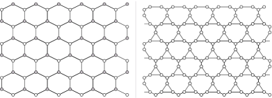
Figure 1: The hexagonal and martini lattices.

The bipartition is indicated by white and grey vertices in Figure 1. Transform the grey vertices from Y to $\Delta$ as in Figure 1 to get the martini lattice. The untransformed vertices form the set $R$.

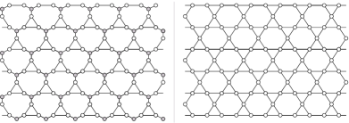
Figure 2: The martini lattice with $R$ in grey. The graph $G^{\prime}$ is the hexagonal dimer lattice.

Replace the vertices of $R$ with cliques to get $G^{\prime}$ as in Figure 2. By Corollary 5.2 the maximal independent sets of $G^{\prime}$ in Figure 2 counts the ground states of the martini lattice. Comparing the hexagonal lattice in Figure 1 with $G^{\prime}$ in Figure 2 one notices that $G^{\prime}$ is the hexagonal dimer lattice. Ending up with the dimer lattice is a general feature of the procedure examplified on the hexagonal lattice. Counting maximal independent sets of the hexagonal dimer lattice is the same as counting perfect matchings on the hexagonal lattice, and that is solved [17, 20].

Now we repeat the same procedure but start off with a 3D-grid with closed boundaries.

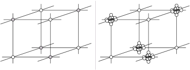
Figure 3: The 3D-grid and the semi-dimer 3D-grid.

A piece of the 3D-grid with a bipartition into white and grey vertices is drawn in Figure 3. Replace every grey vertex with a complete graph of the same order as the vertex degree to get the semi-dimer 3D-grid in Figure 3. By Corollary 5.2 the number of ground states for the semi-dimer 3D-grid is the same as the number of perfect matchings on the 3D-grid, and there are good bounds for those as well [3, 19].

For any lattice obtained from this procedure there is a good lower bound on the number of ground states. It follows from Schrijver’s [19] result that there are at least

$$\left(\frac{(k-1)^{k-1}}{k^{k-2}}\right)^{n/2}$$

perfect matchings on a $k$-regular bipartite graph on $n$ vertices.

 

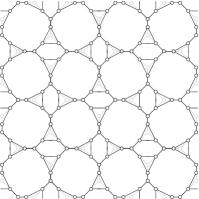
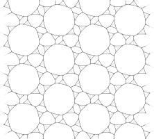
Figure 4: Graphs produced from the edges of the truncated square tiling and the great rhombitrihexagonal tiling [13].

In Figure 4 two graphs produced from 3-regular bipartite graphs are illustrated. According to Schrijver’s bound there are at least $(4/3)^{n/2}$ perfect matchings. We can now construct lattices in arbitrary dimensions with more than $\alpha^{n}$ ground states for $\alpha>1$ according to the following construction. For $d>1$ dimensions let $n_{1},n_{2},\ldots,n_{d}$ be even positive numbers larger than two. Start with the $2d$–regular bipartite graph $T=C_{n_{1}}\times C_{n_{2}}\times\cdots\times C_{n_{d}}$, a $d$-dimensional grid with closed boundaries. Take one of the two parts of $T$ and replace each vertex with $2d$ new vertices as for the 3D-grid. Then we get a $d$-dimensional lattice with at least

$$\left(\frac{(2d-1)^{2d-1}}{(2d)^{2d-2}}\right)^{\frac{n_{1}n_{2}\cdots n_{d}}{2}}$$

ground states.

Acknowledgements

The author thanks Christian Krattenthaler, Philippe Di Francesco, and the Mathematisches Forschungsinstitut Oberwolfach for organizing a week on enumerative combinatorics and statistical mechanics; Anton Dochtermann and Jakob Jonsson for their comments on the paper; and the referees for their suggestions, in particular regarding the connections to the cohomological method and the 3-rule.

References

- [1] M. Bousquet-Mélou, S. Linusson, E. Nevo, On the independence complex of square grids, J. Algebraic Combin., to appear, arXiv:math/0701890.
- [2] A. Björner, Topological Methods, in: “Handbook of Combinatorics” (eds. R. Graham, M. Grötschel, and L. Lovász), North-Holland, 1995, 1819–1872.
- [3] M. Ciucu, An improved upper bound for the -dimensional dimer problem. Duke Math J. 94 (1998), no. 1, 1–11.
- [4] R. Ehrenborg, G. Hetyei, The topology of the independence complex. European J. Combin. 27 (2006), no. 6, 906–923.
- [5] A. Engström, Independence complexes of claw-free graphs. European J. Combin. 29 (2008), no. 1, 234–241
- [6] A. Engström, Complexes of Directed Trees and Independence Complexes, preprint 2005, arXiv:math/0508148
- [7] H. van Eerten, Extensive ground state entropy in supersymmetric lattice models, J. Math. Phys. 46 (2005), no. 12, 123302, 8 pp.
- [8] P. Fendley, J. Halverson, L. Huijse, K. Schoutens, Charge frustration and quantum criticality for strongly correlated fermions, preprint 2008, arXiv:0804.0174
- [9] P. Fendley, K. Schoutens, Exact Results for Strongly Correlated Fermions in 2+1 Dimensions, Phys. Rev. Lett. 95 (2005), 046403, 4 pp.
- [10] P. Fendley, K. Schoutens, J. de Boer, Lattice Models with Supersymmetry, Phys. Rev. Lett. 90 (2003), 120402, 4 pp.
- [11] P. Fendley, K. Schoutens, H. van Eerten, Hard squares with negative activity, J. Phys. A 38 (2005), no. 2, 315–322.
- [12] R. Forman, Morse theory for cell complexes, Adv. Math. 134 (1998), no. 1, 90–145.
- [13] B. Grünbaum, G.C. Shephard, Tilings and patterns. W.H. Freeman and Company, New York, 1989. 446pp.
- [14] L. Huijse, K. Schoutens, Superfrustration of charge degrees of freedom, preprint 2007, arXiv:0709.4120
- [15] J. Jonsson, Hard squares with negative activity and rhombus tilings of the plane, Electron. J. Combin. 13 (2006), no. 1, Research Paper 67, 46 pp.
- [16] J. Jonsson, Simplicial Complexes of Graphs, Lecture Notes in Mathematics, Vol. 1928, Springer, 2008, 378 pp.
- [17] P.W. Kasteleyn, Dimer statistics and phase transitions, J. Mathematical Phys. 4 (1963) 287–293.
- [18] D.N. Kozlov, Complexes of directed trees, J. Combin. Theory Ser. A, 88 (1999), no. 1, 112–122.
- [19] A. Schrijver, Counting -factors in regular bipartite graphs. J. Combin. Theory Ser. B 72 (1998), no. 1, 122–135.
- [20] F.Y. Wu, Remarks on the Modified Potassium Dihydrogen Phosphate Model of a Ferroelectric, Phys. Rev., 168 (1968) 539–543.