Motion of quantum particle in dilute Bose-Einstein condensate at zero temperature

Abstract

The motion of single quantum particle through Bose-Einstein condensate (BEC) is considered within perturbation theory with respect to the particle-BEC interaction. The Hamiltonian of BEC is diagonalized by means of Bogoliubov’s method. The process of dissipation due to the creation of excitation in BEC is analyzed and the dissipation rate is calculated in the lowest order of perturbation theory. The Landau’s criterion for energy dissipation in BEC is then recovered. The energy spectrum of the impurity particle due to the interaction with BEC and its effective mass are evaluated.

I Introduction

Recent experiments on the rotational motion of molecules in the superfluid helium droplets gave rise to a new interest in superfluidity on a microscopic scale vilesov1998 ; vilesov2000 . A unique properties of the measured rotational spectra pose a large number questions, such as: what is the collective molecule/superfluid wavefunction that describes sharp rotational states observed in experiments; what are the properties of finite systems and how is the limit of a bulk superfluid is reached dumesh2006 ? A similar microscopic phenomena were studied in the BEC of Sodium atoms in magnetic traps chikkatur2000 . A linear motion of impurities was shown to be dissipationless for the speeds below the condensate speed of sound. A large number of theoretical works described the molecule/droplet system using imaginary time path integral Monte-Carlo approaches dalfovo2001 ; whaley2004p ; whaley2001k ; whaley2004z ; whaley2004zk ; whaley2003p ; roy2006 . While in certain cases remarkable agreement with experimental constants was obtained roy2006 , those works are strictly limited to the calculation of statistical properties and thus provides no real understanding of the microscopic nature of the dissipationless motion. The latter can only be established by considering a real time dynamics. Several theoretical works considered a motion of impurity through dilute BEC. Recent works considered a macroscopic particle interacting with dilute BEC suzuki2005 . In this case the motion of particle is equivalent to the BEC in a time dependent external potential. This problem was treated by solving time-dependent Gross-Pitaevskii equations astrak2004 . A microscopic particle interacting with the dilute BEC in Bogoliubov’s approximation has been considered by several authors using general Golden rule considerations montina2003 ; montina2002 ; timmermans98 . These works were based on the result of Miller et al miller62 which was obtained using time-independent perturbation theory. The Bogoliubov’s treatment has also been successfully used for the investigation of the force acting on the impurity particle due to the quantum fluctuations in BEC roberts2006 ; roberts2005 . Some authors treated a particle strongly interacting with Bogoliubov’s BEC and found a possibility of self localization kalas2006 ; cucchietti2006 ; sacha2006 .

In this work we attempt to describe impurity moving through BEC as a microscopic particle within time-dependent perturbation theory. We introduce the Hamiltonian of a quantum particle moving within the interacting Bose gas. No assumption is made about the relative mass of an impurity compared to that of the Bose particles. We present the analytic results for this problem in the limit of the dilute Bose gas at zero temperature. After the introduction of the general Hamiltonian, the Bogoliubov’s approximation is made to convert the Hamiltonian to the diagonal form. Then the problem is reduced to the quantum particle moving through the gas of non-interacting Bogoliubov’s excitations. The initial conditions are chosen such that an impurity is not correlated with the BEC. The static properties are achieved after the system reaches thermal equilibrium in a long time limit of our treatment.

We obtain the expansion for the transition amplitude in powers of particle-BEC interaction and restrict ourselves to the calculation of the leading term of this expansion that corresponds to the Golden rule approximation. The latter allows us to calculate various observables such as: state-to-state transition probability, dissipation rate, and the effective mass of the particle. Then we obtain the criterion for the critical momentum of a particle below which its motion becomes non-dissipative, i.e. the microscopic version of the Landau’s criterion. This criterion comes from the exact momentum-energy conservation law. Finally, we calculate the branch of the excitation spectrum corresponding to the moving impurity, i.e. the energy of impurity as a function of its momentum. Expanding the energy at small momenta it is found that the linear part of energy vanishes and the impurity behaves like a free particle with an effective mass that is determined by the second order derivative of energy with respect to momentum. We show that our results agree with a time-independent treatment of Miller within long time limit.

II MODEL HAMILTONIAN

In this section the model for the interacting Bose gas is discussed as well as the approximations that are made in our treatment. The Hamiltonian of interacting Bose particles in coordinate representation is given by

$$H_{B}=-\sum_{\alpha}\frac{1}{2m}\frac{d^{2}}{d{\bf r}_{\alpha}^{2}}+\frac{1}{2}\sum_{\alpha,\beta}U({\bf r}_{\alpha}-{\bf r}_{\beta})~{}.$$ (1)

Here and throughout the paper we set $\hbar=1$. In the secondary quantization the above Hamiltonian reads

$$H_{B}=\sum_{\bf p}\frac{{\bf p}^{2}}{2m}b^{+}_{{\bf p}}b_{{\bf p}}+\frac{1}{2V}\sum_{{\bf p}_{1},{\bf p}_{2},{\bf p}}U({\bf p})b^{+}_{{\bf p}_{1}-{\bf p}}b^{+}_{{\bf p}_{2}+{\bf p}}b_{{\bf p}_{2}}b_{{\bf p}_{1}}~{},$$ (2)

where $U({\bf p})$ is the Fourier transform of the interaction potential

$$U({\bf p})=\int U({\bf r})e^{i{\bf pr}}d{\bf r}~{}.$$ (3)

We will concentrate on the case of dilute gas $r_{0}\ll n^{-1/3}$ where $r_{0}$ is the range of potential on which $U(r)$ differs from zero significantly and $n$ denotes density of gas. So the integral (3) is significant in the domain $p_{0}\leq 1/r_{0}$ while characteristic momenta of particles are of the order of $p_{c}\leq n^{1/3}$. Thus due to diluteness condition $p_{0}\gg p_{c}$, and the Fourier transform of the interaction $U({\bf p})$ in Eq. (2) can be replaced by $U_{0}=\int U({\bf r})d{\bf r}$. The zero Fourier component $U_{0}$ is connected with length of $s$-scattering in first order Born approximation as following

$$a_{s}=\frac{m}{4\pi}U_{0}~{}.$$ (4)

Let us consider degenerate Bose gas at zero temperature. In this case the Hamiltonian (2) can be reduced to the diagonal form with the help of the Bogoliubov’s method bogol1947 . The main assumption of the original treatment is that most of the particles of the degenerate gas stay in the ground state with zero energy and the number of particles with non-zero momentum $N_{{\bf p}\not=0}$ is much less then $N_{0}=N_{{\bf p}=0}$. Thus the creation/annihilation operators $b^{+}_{{\bf p}=0}$ and $b_{{\bf p}=0}$ can be replaced by the macroscopic number $\sqrt{N_{0}}$. So one can expand the interaction part of the Hamiltonian (2) in powers of $\sqrt{N_{{\bf p}\not=0}/N_{0}}$ and leave the terms of expansion up to second order only. After the described procedure the Hamiltonian of the Bose gas attains the form

$$H_{B}=\sum_{\bf p}\frac{p^{2}}{2m}b^{+}_{{\bf p}}b_{{\bf p}}+\frac{U_{0}}{2V}\left[N^{2}-N+N\sum_{{\bf p}\not=0}\left(b^{+}_{\bf p}b^{+}_{\bf-p}+b_{\bf p}b_{\bf-p}+2b^{+}_{\bf p}b_{\bf p}\right)\right]~{},$$ (5)

where $N=N_{0}+N_{{\bf p}\not=0}$. The next step is to diagonalize the Hamiltonian (5) introducing new bosonic creation/annihilation operators $B^{+}_{\bf p}$ and $B_{\bf p}$ related to old operators $b^{+}_{\bf p}$ and $b_{\bf p}$ by linear transformation

$$b_{\bf p}=\alpha_{\bf p}B_{\bf p}+\beta_{\bf p}B^{+}_{\bf-p}~{},~{}~{}~{}\\ b^{+}_{\bf p}=\alpha_{\bf p}B^{+}_{\bf p}+\beta_{\bf p}B_{\bf-p}~{}.$$ (6)

Substituting Eqs. (6) into the Hamiltonian (5) and requiring the Hamiltonian to have diagonal form, one gets for the transformation coefficients landau_v9

$$\alpha_{\bf p} = \frac{\mu_{\bf p}}{\sqrt{\mu_{\bf p}^{2}-1}}~{},~{}~{}~{}\beta_{\bf p}=\frac{1}{\sqrt{\mu_{\bf p}^{2}-1}}~{},~{}~{}~{}$$ (7)

$$\mu_{\bf p} = -\frac{\epsilon({\bf p})+p^{2}/2m+nU_{0}}{nU_{0}}~{},$$

together with the Hamiltonian in new representation

$$H_{B}=E_{0}+\sum_{\bf p}\epsilon(p)B^{+}_{\bf p}B_{\bf p}~{}.$$ (8)

The excitation spectrum $\epsilon(p)$ of the system yields

$$\epsilon(p)=\sqrt{\frac{p^{2}}{2m}\left(\frac{p^{2}}{2m}+2nU_{0}\right)}~{},$$ (9)

and has the phonon-like behavior at low momenta, i.e. $\epsilon(p\to 0)=p\sqrt{nU_{0}/m}=pc$, where $c$ is the speed of sound. The ground state energy of BEC is given by

$$E_{0}=\frac{nU_{0}}{2}(N-1)+\frac{1}{2}\sum_{{\bf p}\not=0}\left(\epsilon(p)-\frac{p^{2}}{2m}-nU_{0}\right)~{}.$$ (10)

Now let us introduce a single quantum particle with mass $M$ and coordinate ${\bf R}$ interacting with the environment of Bose gas discussed above. The whole system is then described by following Hamiltonian

$$H=-\frac{1}{2M}\frac{d^{2}}{d{\bf R}^{2}}+H_{B}+H_{I}$$ (11)

with the particle-environment interaction

$$H_{I}=\frac{g}{V}\sum_{{\bf p},{\bf k}}b_{{\bf p}+{\bf k}}^{+}b_{\bf p}e^{-i{\bf k}{\bf R}}~{}.$$ (12)

Here the coupling constant $g$ is determined as zero Fourier component of the system-environment interaction. In the spirit of Bogoliubov’s theory we expand the interaction Hamiltonian (12) in powers of $\sqrt{N_{{\bf p}\not=0}/N_{0}}$ and leave the terms of zeroth and first order, i.e. leading terms. Then the Hamiltonian (12) takes the form

$$H_{I}=gn+\frac{g\sqrt{N}}{V}\sum_{{\bf p}\not=0}\left(b_{\bf p}^{+}e^{-i{\bf p}{\bf R}}+b_{{\bf p}^{\prime}}e^{i{\bf p}{\bf R}}\right)~{}.$$ (13)

We neglected the terms of the order of $N_{p\not=0}$ in (13). As it becomes clear below, the contribution of the higher order terms to the dissipation process is of the order of $N_{{\bf p}\not=0}$ which would be an excess precision compared with the Bogoliubov’s approximation made above. Expressing operators $b_{\bf p}^{+}$ and $b_{\bf p}$ through new operators $B_{\bf p}^{+}$ and $B_{\bf p}$, and using the secondary quantization representation for the system particle, for the full Hamiltonian (11) one gets

$$H = E^{\prime}_{0}+\sum_{\bf q}\frac{{\bf q}^{2}}{2M}a_{\bf q}^{+}a_{\bf q}+\sum_{\bf p}\epsilon(p)B^{+}_{\bf p}B_{\bf p}+\sum_{{\bf q},{\bf p}\not=0}\gamma_{\bf p}\left(a^{+}_{{\bf q}-{\bf p}}a_{\bf q}B^{+}_{\bf p}+a^{+}_{{\bf q}+{\bf p}}a_{\bf q}B_{\bf p}\right)~{},$$ (14)

$$\gamma_{\bf p} = \frac{g}{V}\sqrt{\frac{Np^{2}}{2m\epsilon(p)}}~{}.$$

Here operators $a^{+}_{\bf q}/a_{\bf q}$ create/annihilate the particle in state $|{\bf q}\rangle$, and the ground state energy $E_{0}^{\prime}=E_{0}+gn$ is shifted with respect to the $E_{0}$ due to the system-condensate interaction.

III TRANSITION PROBABILITY AND DISSIPATION RATE

The next step is the calculation of the transition probability for the whole system from some initial state $|i\rangle$ to final state $|f\rangle$. So our aim is to construct the perturbative expansion for the matrix element of the evolution operator $a_{if}(t)=\langle f|e^{-iHt}|i\rangle$ in powers of particle-BEC interaction (13). Here we restrict ourselves to the calculation of the leading, i.e. lowest order term of this expansion only. Let us write the matrix element of evolution operator in interaction representation

$$a_{if}(t) = \langle f|e^{-iH_{0}t}{\rm T}\exp\left(-i\int_{0}^{t}H_{I}(s){\rm d}s\right)|i\rangle~{},$$ (15)

$$H_{0} = H-H_{I}~{},~{}~{}~{}H_{I}(s)=e^{iH_{0}s}H_{I}e^{-iH_{0}s}~{}.$$ (16)

Initial and final states of the system particle are supposed to be free particle states $|{\bf q}\rangle=\frac{1}{\sqrt{V}}e^{i{\bf q}{\bf R}}$ with momenta ${\bf q}_{i}$ and ${\bf q}_{f}$, respectively. The Bose environment is initially in its ground state $|0\rangle_{B}$ and then evolutes into some final state $|f\rangle_{B}$. Note that the state $|0\rangle_{B}$ is the ground state of the diagonalized Hamiltonian (8) with the ground state energy $E^{\prime}_{0}$ and it does not equal the state in which all of the Bose particles have zero momentum. Below we will find the transition amplitude as an expansion in powers of coupling constant $g$, i.e.

$$a_{if}(t)=a_{if}^{(0)}(t)+a_{if}^{(1)}(t)+a_{if}^{(2)}(t)+...~{},~{}~{}~{}a_{if}^{(n)}(t)\sim g^{n}~{}.$$ (17)

The zeroth order term is given by $a_{if}^{(0)}(t)=\delta_{{\bf q}_{f},{\bf q}_{i}}\exp\left[-i(E_{0}^{\prime}-q_{i}^{2}/2M)t\right]$. The first order term of expansion describes the process of creation of excitation in BEC with the momentum ${\bf p}_{f}$ due to the interaction with the particle

$$a_{if}^{(1)}(t)=-i\int_{0}^{t}ds\sum_{{\bf p},{\bf q}}\gamma_{\bf p}\langle{\bf p}_{f}|_{B}\langle{\bf q}_{f}|e^{-iH_{0}(t-s)}a^{+}_{{\bf q}-{\bf p}}a_{\bf q}B^{+}_{\bf p}e^{-iH_{0}s}|{\bf q}_{i}\rangle|0\rangle_{B}$$

$$=-i\gamma_{{\bf p}_{f}}\delta_{{\bf q}_{f},{\bf q}_{i}-{\bf p}_{f}}\int_{0}^{t}ds\exp\left[-i\left(E_{0}^{\prime}-q_{i}^{2}/2M\right)t-i\omega({\bf p})(t-s)\right]~{},$$ (18)

where $\omega({\bf p})=\epsilon(p)+p^{2}/2M-{\bf q}_{i}{\bf p}/M~{}$. The term of second order is defined by two processes: first, is creation of two excitation in BEC; and second, is creation and annihilation of one excitation in BEC while the particle finally remains in its initial state. We will consider the amplitude of the latter process since only this amplitude gives the contribution of second order into the transition probability. Thus the second order matrix element reads

$$a_{if}^{(2)}(t)=-\frac{1}{2}\int_{0}^{t}ds\int_{0}^{t}ds\prime\langle 0|_{B}\langle{\bf q}_{f}|e^{-iH_{0}t}{\rm T}\left(H_{I}(s)H_{I}(s^{\prime})\right)|{\bf q}_{i}\rangle|0\rangle_{B}$$

$$=-\delta_{{\bf q}_{f},{\bf q}_{i}}\sum_{\bf p}\int_{0}^{t}ds\int_{0}^{t}ds^{\prime}\Theta(s-s^{\prime})\exp\left[-i\left(E_{0}^{\prime}-q_{i}^{2}/2M\right)t-i\omega({\bf p})(s-s^{\prime})\right]~{}.$$ (19)

Finally, one can find the probability of the particle transition from state $|{\bf q}_{i}\rangle$ to $|{\bf q}_{f}\rangle$ in the following form

$$w_{if}=\delta_{{\bf q}_{i},{\bf q}_{f}}\left(1-\sum_{\bf p}\gamma_{\bf p}^{2}\left|\int_{0}^{t}dse^{-is\omega({\bf p})}\right|^{2}\right)+\gamma^{2}_{{\bf q}_{i}-{\bf q}_{f}}\left|\int_{0}^{t}dse^{-is\omega({\bf q}_{i}-{\bf q}_{f})}\right|^{2}~{}.$$ (20)

The standard way to deal with the integral $\int_{0}^{t}dse^{-i\omega s}$ in the expression for the transition probability (20) is to evaluate its value in the limit of long time interval $t\gg 1/\omega$. So for the square of the absolute value of this integral one gets

$$\left|\int_{0}^{t}dse^{-is\omega({\bf p})}\right|_{t\to\infty}^{2}\longrightarrow~{}2\pi t\delta(\omega({\bf p}))~{}.$$ (21)

First, let us discuss the probability of the particle of leaving its initial state $|{\bf q}_{i}\rangle$ and moving to the state with a different arbitrary momentum $|{\bf q}_{f}\rangle$ in a unit of time with creation of the Bogoliubov’s excitation in the surrounding BEC with the momentum ${\bf p}={\bf q}_{f}-{\bf q}_{i}$. In the long time approximation the probability reads

$$dw({\bf p})=2\pi\gamma_{\bf p}^{2}\delta(\omega({\bf p}))dt~{}.$$ (22)

So the maximum momentum $p_{M}$ that can be transmitted from particle to BEC is collinear to ${\bf q}_{i}$ and determined by the crossing point of the line $q_{i}p/M$ and the curve $\epsilon(p)+p^{2}/2M$

$$p_{M}=\frac{2}{1-(M/m)^{2}}\left(q_{i}-\sqrt{q_{c}^{2}+(M/m)^{2}(q_{i}^{2}-q_{c}^{2})}\right),~{}~{}~{}q_{c}=Mc~{}.$$ (23)

Besides, the maximum angle $\theta_{M}$ between vectors ${\bf q}_{i}$ and ${\bf p}$ is given by the condition $\cos\theta_{M}=q_{c}/q_{i}$. Thus we have the Cherenkov like emission of the BEC excitation with the length of the momentum $0<|{\bf p}|<p_{M}$ into the cone with the angle $\theta_{m}$ along the vector ${\bf q}_{i}$.

Next, we can define the transition rate as the probability of the particle to leave its initial state $|{\bf q}_{i}\rangle$ in a unit of time as

$$\Gamma_{T}=\sum_{\bf p}\frac{dw(\omega({\bf p}))}{dt}$$ (24)

In the thermodynamic limit ($N\to\infty,~{}~{}V\to\infty,~{}~{}N/V=n$) one has to replace the sum over momenta $\sum_{\bf p}$ by the integral $\frac{V}{(2\pi)^{3}}\int d{\bf p}$ in the right hand side of Eq. (24), and for the transition rate one gets

$$\Gamma_{T}=\frac{ng^{2}}{8\pi^{2}m}\int d{\bf p}\frac{p^{2}}{\epsilon(p)}\delta(\omega({\bf p}))~{}.$$ (25)

Let us write the integral in Eq. (25) in the following form

$$\Gamma_{T}=\frac{nMg^{2}}{4\pi mq_{i}}\int_{0}^{\infty}dp\frac{p^{3}}{\epsilon(p)}\int_{0}^{1}dx\delta(x-x_{0})~{},$$ (26)

where $x={\bf p}{\bf q}_{i}/pq_{i}$ and the value $x_{0}$ is determined from the condition $\omega({\bf p})=0$. So the integral over $x$ is unit only if $x_{0}<1$, or

$$\epsilon(p)+p^{2}/2M<pq_{i}/M~{}.$$ (27)

Clearly the condition (27) is never fulfilled if the absolute value of the initial momentum of the particle $q_{i}$ is less then $M\epsilon(p\to 0)/p=Mc=p_{c}$, and then the integral in the expression for the transition rate $\Gamma_{T}$ is always zero. At this point we recovered the Landau’s criterion - there is no energy dissipation if the speed of particle $v_{i}=q_{i}/M$ moving through the interacting Bose gas is less than speed of sound.

To evaluate the rate for momenta above the critical one we proceed further with the integral (26)

$$\Gamma_{T}=\frac{nMg^{2}}{4\pi mq_{i}}\int_{0}^{p_{M}}dp\frac{p^{3}}{\epsilon(p)}~{}.$$ (28)

Here the integration is performed over momentum $p$ from zero to the crossing point $p=p_{M}$ given by Eq. (23). Finally, the transition rate reads

$$\Gamma_{T}=\frac{Mmng^{2}}{2\pi q_{i}}\left[\epsilon(p_{M})-mc^{2}\ln\left(1+\frac{\epsilon(p_{M})+p_{M}^{2}/2m}{mc^{2}}\right)\right]~{}.$$ (29)

Let us consider the limit case when the initial momentum $q_{i}$ is close to its critical value $q_{c}$. Expanding the expression (23) in powers of small $q_{i}-q_{c}$ and assuming the value $M/m$ to be finite, for the upper limit of integration we obtain $p_{M}\approx 2(q_{i}-q_{c})$. Then expanding the right hand side of Eq.(29) in powers of $p_{M}/mc$, for the leading term of expansion one gets

$$\Gamma_{T}(q_{i}\sim q_{c})=\frac{2ng^{2}}{3\pi mc^{2}}(q_{i}-q_{c})^{3}~{}.$$ (30)

So the lowest term of expansion appears to be of the third order of small value $q_{i}-q_{c}$. In the opposite case of large initial momentum $q_{i}\gg q_{c}$ one can obtain the following expression for the transition rate

$$\Gamma_{T}=\frac{ng^{2}Mq_{i}}{\pi}\left(\frac{m}{M+m}\right)^{2}~{},$$ (31)

which is surely independent on speed of sound.

Our next example is the calculation of the energy transferred from particle to BEC as a function of time

$$E(t)=\sum_{\bf p}\epsilon(p)\gamma^{2}_{\bf p}\left|\int_{0}^{t}dse^{-is\omega({\bf p})}\right|^{2}_{t\to\infty}=2\pi t\frac{V}{(2\pi)^{3}}\int d{\bf p}\gamma_{\bf p}^{2}\epsilon(p)\delta(\omega({\bf p}))~{}.$$ (32)

Here we can determine the dissipation rate as the amount of energy transferred in unit of time

$$\Gamma_{E}=\frac{dE(t)}{dt}=\frac{ng^{2}}{8\pi^{2}m}\int d{\bf p}p^{2}\delta(\omega({\bf p}))~{}.$$ (33)

Calculating the integral in (33) in the same manner as described above, for the dissipation rate one gets

$$\Gamma_{E}=\frac{Mng^{2}p_{M}^{4}}{16\pi mq_{i}}~{}.$$ (34)

In the limit case of massive particle $M\gg m$ the expression (34) converges to the following value

$$\Gamma_{E}=\frac{ng^{2}(q_{i}^{2}-q_{c}^{2})^{2}}{\pi q_{i}}\left(\frac{m}{M}\right)^{3}~{}.$$ (35)

This result exactly corresponds to the rate of energy dissipation obtained in suzuki2005 for the classical particle moving through BEC with constant velocity.

IV PARTICLE ENERGY SPECTRUM AND EFFECTIVE MASS

In this section we will consider the non-dissipative motion of the impurity though the BEC when the initial momentum of the impurity particle $q_{i}$ is less than the critical momentum $q_{c}=Mc$ at which the dissipation process occurs according to the Landau’s criterium. In the absence of dissipation one would expect that the impurity will move as a free particle but its energy should be shifted due to the coupling with the BEC environment. Thus our purpose is to calculate the contribution to the energy of the impurity due to the interaction with BEC and the effective mass of the particle.

Let us start with the calculation of the full energy of the particle-BEC system as a function of time. Following the perurbative treatment developed above, one can write the energy of the system as an expansion in powers of coupling parameter $g$

$$E(t)=E^{(0)}(t)+E^{(1)}(t)+E^{(2)}(t)~{},$$ (36)

coming from the expansion for the evolution of density matrix

$$\rho(t)=\rho^{(0)}(t)+\rho^{(1)}(t)+\rho^{(2)}(t)~{}.$$ (37)

The system energy as a function of time is then given by $E(t)={\rm Tr}\left(H\rho(t)\right)$, where $H$ is the Hamiltonian of the full system (14) and ${\rm Tr}$ denotes the trace over all possible states. The zeroth order contribution corresponding to the unperturbed system is

$$E^{(0)}={\rm Tr}\left(H_{0}\rho^{(0)}\right)=E_{0}^{\prime}+\frac{q_{i}^{2}}{2M}~{}.$$ (38)

The first order does not bring any contribution since ${\rm Tr}\left(H_{0}\rho^{(1)}(t)+H_{I}\rho^{(0)}(t)\right)=0$. The second order term consists of two terms $E^{(2)}={\rm Tr}\left(H_{0}\rho^{(2)}\right)+{\rm Tr}\left(H_{I}\rho^{(1)}\right)$. Let us consider the first term

$${\rm Tr}\left(H_{0}\rho^{(2)}\right)=\sum_{f}w^{(2)}_{i,f\not=i}\left(\frac{q_{f}^{2}}{2M}+\epsilon(p_{f})+E_{0}^{\prime}\right)+w^{(2)}_{i,f=i}\left(\frac{q_{i}^{2}}{2M}+E_{0}^{\prime}\right)~{},$$ (39)

where the transition probability $w_{if}^{(2)}$ is defined by Eq. (20) as $w^{(2)}_{if}=w_{if}-1$. We are interested again in the long time limit when the whole system reaches its equilibrium state, so the upper limit of integration over time in the right hand side of Eq. (20) must be replaced by infinity. Since here we consider the case of dissipationless motion of the impurity, $\omega({\bf p})\not=0$ and instead of the limit (21) one has to use following formula

$$\left|\int_{0}^{t}dse^{-is\omega({\bf p})}\right|_{t\to\infty}^{2}\longrightarrow\frac{1}{\omega^{2}({\bf p})}~{}.$$ (40)

Hence for the term (39) we have

$${\rm Tr}\left(H_{0}\rho^{(2)}\right)=\sum_{\bf p}\frac{\gamma^{2}_{\bf p}}{\omega({\bf p})}~{}.$$ (41)

The remaining term ${\rm Tr}\left(H_{I}\rho^{(1)}\right)$ is given by

$${\rm Tr}\left(H_{I}\rho^{(1)}\right)=\sum_{f\not=i}\left(\langle f|H_{I}|i\rangle\langle i|\rho^{(1)}(t)|f\rangle~{}+~{}c.c.\right)~{}.$$ (42)

Using the expression for the interaction Hamiltonian Eq. (13) and noting that $\langle i|\rho^{(1)}(t)|f\rangle=a_{if}^{(0)}(t)a_{if}^{(1)*}(t)$, for the above term one gets

$${\rm Tr}\left(H_{I}\rho^{(1)}\right)=-2\sum_{\bf p}\gamma_{\bf p}^{2}\int_{0}^{t}ds\sin(s\omega({\bf p}))~{}.$$ (43)

In the long time limit $\int_{0}^{\infty}ds\sin(s\omega({\bf p}))={\mathcal{P}}\frac{1}{\omega({\bf p})}$, where ${\mathcal{P}}$ denotes principal value. Finally, the energy shift given by the sum of terms (39) and (43) reads

$$E^{(2)}=-\sum_{\bf p}\frac{\gamma^{2}_{\bf p}}{\omega({\bf p})}=-\frac{ng^{2}}{16\pi^{3}m}\int d{\bf p}\frac{p^{2}}{\epsilon(p)\omega({\bf p})}~{}.$$ (44)

As was mentioned above, here we are interested in evaluation of the energy of the impurity particle in case of relatively small initial momentum $q_{i}$. In this case the energy can be written as an expansion in powers of small parameter $q_{i}/q_{c}$ up to second order, i.e.

$$E_{p}(q_{i})=E_{p}(0)+\frac{q_{i}^{2}}{2M_{ef}}~{}.$$ (45)

It turns out that the term linear in $q_{i}$ disappears, and the effective mass of the particle in (45) is determined as follows

$$\frac{1}{M_{ef}}=\frac{1}{M}+\left.\frac{d^{2}E^{(2)}}{dq_{i}^{2}}\right|_{q_{i}=0}~{}.$$ (46)

Let us start with the calculation of the zeroth order contribution in powers of $q_{i}$

$$E_{p}(0)=ng-\frac{1}{4\pi^{2}}\frac{ng^{2}}{m}\int_{0}^{\infty}\frac{p^{4}dp}{\epsilon(p)\big{(}\epsilon(p)+p^{2}/2M\big{)}}~{}.$$ (47)

The integral in the right hand side of Eq. (47) diverges at large momentum like $4mm_{r}\int_{0}^{\infty}dp$, where $m_{r}=\left(1/m+1/M\right)^{-1}$ is reduced mass of the system of the relevant and the BEC particles. The standard way to avoid the such kind of divergence is to renormalize the coupling constant introducing some another expansion parameter. Let us determine the coupling parameter $g$ as an expansion in powers of scattering length $a$

$$g=\frac{2\pi a}{m_{r}}(1+\kappa a+...)~{},$$ (48)

and then remove the divergence from the expansion for the energy (47) to the expansion (48). Substituting equation (48) into Eq. (47), leaving terms up to second order in powers of scattering length $a$ and requiring the energy $E_{p}(0)$ to be finite, for the renormalized coupling constant one gets

$$g=\frac{2\pi a}{m_{r}}\left(1+\frac{2a}{\pi}\int_{0}^{\infty}dp\right)~{}.$$ (49)

The actual physical reason of the divergence is that the zero Fourier component of the interaction is used as the coupling constant $g$. The procedure of renormalization of coupling constant corresponds to taking into account the second order Born approximation and can also be done employing direct expansion of the scattering length in powers of coupling constant landau_v9 . Using the relation (49), the energy $E_{p}(0)$ is now finite and reads

$$E_{p}(0) = \frac{2\pi na}{m_{r}}\left[1+\frac{4amc}{\pi}I_{0}\left(\frac{m}{M}\right)\right]~{},$$ (50)

$$I_{0}(x) = \frac{x\sqrt{x^{2}-1}-\ln(x+\sqrt{x^{2}-1})}{(x-1)\sqrt{x^{2}-1}}~{}.$$

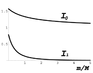
Figure 1: Integrals $I_{0}$ and $I_{1}$ as the functions of relation $m/M$ .

Evaluating the term of the second order expansion in the expression for the energy (44)

$$\left.\frac{d^{2}E^{(2)}}{dq_{i}^{2}}\right|_{q_{i}=0}=-\frac{2}{3}\frac{na^{2}}{mm_{r}^{2}M^{2}}\int_{0}^{\infty}\frac{p^{6}dp}{\epsilon(p)\big{(}\epsilon(p)+p^{2}/2M\big{)}^{3}}~{},$$ (51)

for the effective mass of the particle we have

$$M_{ef}=M\left[1-\frac{32}{3}\frac{na^{2}}{Mc(m_{r}/m)^{2}}I_{1}\left(\frac{m}{M}\right)\right]^{-1}~{},$$ (52)

where

$$I_{1}(y)=\frac{1}{2(y^{2}-1)^{5/2}}\left[(1+2y^{2})\ln(y+\sqrt{y^{2}-1})-3y\sqrt{y^{2}-1}\right]~{}.$$ (53)

The behavior of the functions $I_{0}$ and $I_{1}$ in expressions for the energy (50) and the effective mass (52), respectively, is shown in Fig. (1). In case of heavy particle $M\gg m$ its effective mass yields $M_{ef}=M(1-8\pi na^{2}/3Mc)^{-1}$, the same result as was obtained in navez1999 .

V CONCLUSION

The goal of this paper is the understanding of the effect of superfluidity reflected on a motion of a microscopic impurity inside a BEC environment. Quantitatively our system is very different from the realistic liquid helium. However, for dilute BEC we obtained physical behavior that gives qualitative understanding of manifestation superfluidity on a microscopic scale. We calculated the transition amplitude to the second order of the perturbation theory. The inelastic contribution to this amplitude responsible for the dissipation comes from the first order of the perturbation expansion. It is shown that at the velocities less than speed of sound this term is zero and we recover the exact Landau’s criterion. The elastic part corresponds to the second order term and is responsible for the shift of the particle energy. Divergence of this energy shift which appears because of the delta-functional potential is avoided by renormalization of coupling constant. The energy of the particle is calculated as a function of its momentum. At small momenta this function is quadratic, thus the impurity moves like a free particle but its mass is shifted due to the interaction with the BEC. The natural extension of this work is the calculation of the Green’s function of an impurity and the development of the perturbation theory for its poles. This work is currently in progress.

VI ACKNOWLEDGEMENTS

The support for this work has been provided by the NSF (CAREER award no. 0645340) and by the University of Rochester.

References

- (1) E. M. Lifshitz and L. P. Pitaevskii, Statistical Physics, Part 2, Pergamon Press, Oxford, 1980.
- (2) N. N. Bogoliubov, J. Phys. (Moscow) 11 (1947) 23
- (3) Jun Suzuki, arXiv: cond-mat/0407714 (2005).
- (4) G. E. Astrakharchik and L. P. Pitaevskii, Phys. Rev. A 70 (2004) 013608.
- (5) P. Navez and M. Wilkens, J. Phys. B: At. Mol. Opt. Phys. 32 (1999) L629.
- (6) S. Grebenev, P. Toennis and A. Vilesov, Science 279 (1998) 2083.
- (7) S. Grebenev, B. Sartakov, P. Toennis and A. Vilesov, Science 289 (2000) 1532.
- (8) B. S. Dumesh and L. A. Surin, Physics-Uspekhi 49 (2006) 11
- (9) F. Dalfovo and S. Stringary, J. Chem. Phys. 115 (2001) 10078
- (10) F. Paesani and K. B. Whaley, J. Chem. Phys. 121 (2004) 5293
- (11) Y. Kwon and K. B. Whaley, J. Chem. Phys. 114 (2001) 3163
- (12) R. E. Zillich and K. B. Whaley, Phys. Rev. B 69 (2004) 104517
- (13) R. E. Zillich, Y. Kwon and K. B. Whaley, Phys. Rev. Lett. 93 (2004) 250401
- (14) M. V. Patel, A. Viel, F. Paesani, P. Huang and K. B. Whaley, J. Chem. Phys. 118 (2003) 5011
- (15) W. Topic, W. Jaeger, N. Blinov, P.-N. Roy, M. Botti, and S. Moroni, J. Chem. Phys. 125 (2006) 144310
- (16) R. Kalas and D. Blume, Phys. Rev. A 73 (2006) 043608
- (17) F. M. Cucchietti and E. Timmermans, Phys. Rev. Lett. 96 (2006) 210401
- (18) K. Sacha and E. Timmermans, Phys. Rev. A 73 (2006) 063604
- (19) A. Montina, Phys. Rev. A 67 (2003) 053614
- (20) A. Montina, Phys. Rev. A 66 (2002) 023609
- (21) E. Timmermans and R. Cote, Phys. Rev. Lett. 80 (1998) 3419
- (22) A. Miller, D. Pines and P. Nozieres, Phys. Rev. 127 (1962) 1452
- (23) A. P. Chikkatur, A. Görlitz, D. M. Stamper-Kurn, S. Inouye, S. Gupta and W. Ketterle, Phys. Rv. Lett. 85 (2000) 483
- (24) D. C. Roberts, Phys. Rev. A 74 (2006) 013613
- (25) D. C. Roberts and Y. Pomenau, Phys. Rev. Lett. 95 (2005) 145303