Abstract

We consider the problem of estimating the support of a vector $\beta^{*}\in\mathbb{R}^{p}$ based on observations contaminated by noise. A significant body of work has studied behavior of $\ell_{1}$-relaxations when applied to measurement matrices drawn from standard dense ensembles (e.g., Gaussian, Bernoulli). In this paper, we analyze sparsified measurement ensembles, and consider the trade-off between measurement sparsity, as measured by the fraction $\gamma$ of non-zero entries, and the statistical efficiency, as measured by the minimal number of observations $n$ required for exact support recovery with probability converging to one. Our main result is to prove that it is possible to let $\gamma\rightarrow 0$ at some rate, yielding measurement matrices with a vanishing fraction of non-zeros per row while retaining the same statistical efficiency as dense ensembles. A variety of simulation results confirm the sharpness of our theoretical predictions.

Keywords: Quadratic programming; Lasso; subset selection; consistency; thresholds; sparse approximation; signal denoising; sparsity recovery; $\ell_{1}$-regularization; model selection

1 Introduction

Recent years have witnessed a flurry of research on the recovery of high-dimensional sparse signals (e.g., compressed sensing [2, 6, 18], graphical model selection [13, 14], and sparse approximation [18]). In all of these settings, the basic problem is to recover information about a high-dimensional signal $\beta^{*}\in{\mathbb{R}}^{p}$, based on a set of $n$ observations. The signal $\beta^{*}$ is assumed a priori to be sparse: either exactly $k$-sparse, or lying within some $\ell_{q}$-ball with $q<1$. A large body of theory has focused on the behavior of various $\ell_{1}$-relaxations when applied to measurement matrices drawn from the standard Gaussian ensemble [6, 2], or more general random ensembles satisfiying mutual incoherence conditions [13, 20].

These standard random ensembles are dense, in that the number of non-zero entries per measurement vector is of the same order as the ambient signal dimension. Such dense measurement matrices are undesirable for practical applications (e.g., sensor networks), in which it would be preferable to take measurements based on sparse inner products. Sparse measurement matrices require significantly less storage space, and have the potential for reduced algorithmic complexity for signal recovery, since many algorithms for linear programming, and conic programming more generally [1], can be accelerated by exploiting problem structure. With this motivation, a body of past work (e.g. [4, 8, 16, 23]), motivated by group testing or coding perspectives, has studied compressed sensing methods based on sparse measurement ensembles. However, this body of work has focused on the case of noiseless observations.

In contrast, this paper focuses on observations contaminated by additive noise which, as we show, exhibits fundamentally different behavior than the noiseless case. Our interest is not on sparse measurement ensembles alone, but rather in understanding the trade-off between the degree of measurement sparsity, and its statistical efficiency. We assess measurement sparsity in terms of the fraction $\gamma$ of non-zero entries in any particular row of the measurement matrix, and we define statistical efficiency in terms of the minimal number of measurements $n$ required to recover the correct support with probability converging to one. Our interest can be viewed in terms of experimental design: more precisely we ask: what degree of measurement sparsity can be permitted without any compromise in the statistical efficiency? To bring sharp focus to the issue, we analyze this question for exact subset recovery using $\ell_{1}$-constrained quadratic programming, also known as the Lasso in the statistics literature [3, 17], where past work on dense Gaussian measurement ensembles [20] provides a precise characterization of its success/failure. We characterize the density of our measurement ensembles with a positive parameter $\gamma\in(0,1]$, corresponding to the fraction of non-zero entries per row. We first show that for all fixed $\gamma\in(0,1]$, the statistical efficiency of the Lasso remains the same as with dense measurement matrices. We then prove that it is possible to let $\gamma\rightarrow 0$ at some rate, as a function of the sample size $n$, signal length $p$ and signal sparsity $k$, yielding measurement matrices with a vanishing fraction of non-zeroes per row while requiring exactly the same number of observations as dense measurement ensembles. In general, in contrast to the noiseless setting [23], our theory still requires that the average number of non-zeroes per column of the measurement matrix (i.e., $\gamma n$) tend to infinity; however, under the loss function considered here (exact signed support recovery), we prove that no method can succeed with probability one if this condition does not hold. The remainder of this paper is organized as follows. In Section 2, we set up the problem more precisely, state our main result, and discuss some of its implications. In Section 3, we provide a high-level outline of the proof.

Work in this paper was presented in part at the International Symposium on Information Theory in Toronto, Canada (July, 2008). We note that in concurrent and complementary work, Wang et al. [22] have analyzed the information-theoretic limitations of sparse measurement matrices for exact support recovery.

Notation:

Throughout this paper, we use the following standard asymptotic notation: $f(n)=\mathcal{O}(g(n))$ if $f(n)\leq Cg(n)$ for some constant $C<+\infty$; $f(n)=\Omega(g(n))$ if $f(n)\geq cg(n)$ for some constant $c>0$; and $f(n)=\Theta(g(n))$ if $f(n)=\mathcal{O}(g(n))$ and $f(n)=\Omega(g(n))$.

2 Problem set-up and main result

We begin by setting up the problem, stating our main result, and discussing some of their consequences.

2.1 Problem formulation

Let $\beta^{*}\in{\mathbb{R}}^{p}$ be a fixed but unknown vector, with at most $k$ non-zero entries ($k\leq\frac{p}{2}$), and define its support set

$${S} := \{i\in\{1,\ldots,p\}\,\mid\;\beta^{*}_{i}\neq 0\}.$$ (1)

We use $\beta_{min}$ to denote the minimum value of $|\beta^{*}|$ on its support—that is, $\beta_{min}:=\min_{i\in{S}}|\beta^{*}_{i}|$.

Suppose that we make a set $\{{{Y}}_{1},\ldots,{{Y}}_{n}\}$ of $n$ independent and identically distributed (i.i.d.) observations of the unknown vector $\beta^{*}$, each of the form

$${{Y}}_{i} := x_{i}^{T}\beta^{*}+{{W}}_{i},$$ (2)

where ${{W}}\sim\mathcal{N}(0,\sigma^{2})$ is observation noise, and $x_{i}\in{\mathbb{R}}^{p}$ is a measurement vector. It is convenient to use ${{Y}}=\begin{bmatrix}{{Y}}_{1}&{{Y}}_{2}&\ldots&{{Y}}_{n}\end{bmatrix}^{T}$ to denote the $n$-vector of measurements, with similar notation for the noise vector ${{W}}\in{\mathbb{R}}^{n}$, and

$$X = \begin{bmatrix}x_{1}^{T}\\ x_{2}^{T}\\ \vdots\\ x_{n}^{T}\end{bmatrix}\;=\;\begin{bmatrix}X_{1}&X_{2}&\ldots&X_{p}\end{bmatrix}.$$ (3)

to denote the $n\times p$ measurement matrix. With this notation, the observation model can be written compactly as ${{Y}}=X\beta^{*}+{{W}}$.

Given some estimate $\widehat{\beta}$, its error relative to the true $\beta^{*}$ can be assessed in various ways, depending on the underlying application of interest. For applications in compressed sensing, various types of $\ell_{q}$ norms (i.e., ${\mathbb{E}}\|\widehat{\beta}-\beta^{*}\|_{q}$) are well-motivated, whereas for statistical prediction, it is most natural to study a predictive loss (e.g., ${\mathbb{E}}\|X\widehat{\beta}-X\beta^{*}\|$). For reasons of scientific interpretation or for model selection purposes, the object of primary interest is the support ${S}$ of $\beta^{*}$. In this paper, we consider a slightly stronger notion of model selection: in particular, our goal is to recover the signed support of the unknown $\beta^{*}$, as defined by the $p$-vector ${S}(\beta^{*})$ with elements

$$[{{S}}(\beta^{*})]_{i} := \begin{cases}\operatorname{sign}(\beta^{*}_{i})&\mbox{if $\beta^{*}_{i}\neq 0$}\\ 0&\mbox{otherwise.}\end{cases}$$

Given some estimate $\widehat{\beta}$, we study the probability $\mathbb{P}[{{S}}(\widehat{\beta})={{S}}(\beta^{*})]$ that it correctly specifies the signed support.

The estimator that we analyze is $\ell_{1}$-constrained quadratic programming (QP), also known as the Lasso [17] in the statistics literature. The Lasso generates an estimate $\widehat{\beta}$ by solving the regularized QP

$$\widehat{\beta} = \arg\min_{\beta\in{\mathbb{R}}^{p}}\left\{\frac{1}{2n}\|{{Y}}-X\beta\|_{2}^{2}+\rho_{n}\|\beta\|_{1}\right\},$$ (4)

where $\rho_{n}>0$ is a user-defined regularization parameter. A large body of past work has focused on the behavior of the Lasso for both deterministic and random measurement matrices (e.g., [5, 13, 18, 20]). Most relevant here is the sharp threshold [20] characterizing the success/failure of the Lasso when applied to measurement matrices $X$ drawn randomly from the standard Gaussian ensemble (i.e., each element $X_{ij}\sim\mathcal{N}(0,1)$ i.i.d.). In particular, the Lasso undergoes a sharp threshold as a function of the control parameter

$$\theta(n,p,k) := \frac{n}{2k\log(p-k)}.$$ (5)

For the standard Gaussian ensemble and sequences $(n,p,k)$ such that $\theta(n,p,k)>1$, the probability of Lasso success goes to one, whereas it converges to zero for sequences for which $\theta(n,p,k)<1$. The main contribution of this paper is to show that the same sharp threshold holds for $\gamma$-sparsified measurement ensembles, including a subset for which $\gamma\rightarrow 0$, so that each row of the measurement matrix has a vanishing fraction of non-zero entries.

2.2 Statement of main result

A measurement matrix $X\in{\mathbb{R}}^{n\times p}$ drawn randomly from a Gaussian ensemble is dense, in that each row has $\Theta(p)$ non-zero entries. The main focus of this paper is the observation model (2), using measurement ensembles that are designed to be sparse. To formalize the notion of sparsity, we let $\gamma\in(0,1]$ represent a measurement sparsity parameter, corresponding to the (average) fraction of non-zero entries per row. Our analysis allows the sparsity parameter $\gamma(n,p,k)$ to be a function of the triple $(n,p,k)$, but we typically suppress this explicit dependence so as to simplify notation. For a given choice of $\gamma$, we consider measurement matrices $X$ with i.i.d. entries of the form

$$X_{ij} \stackrel{{\scriptstyle d}}{{=}} \begin{cases}Z\sim\mathcal{N}(0,1)&\mbox{with probability $\gamma$}\\ 0&\mbox{with probability $1-\gamma$}.\end{cases}$$ (6)

By construction, the expected number of non-zero entries in each row of $X$ is $\gamma p$. It is straightforward to verify that for any constant setting of $\gamma$, elements $X_{ij}$ from the ensemble (6) are sub-Gaussian. (A zero-mean random variable $Z$ is sub-Gaussian [19] if there exists some constant $C>0$ such that $\mathbb{P}[|Z|>t]\leq 2\exp(-Ct^{2})$ for all $t>0$.) For this reason, one would expect such ensembles to obey similar scaling behavior as Gaussian ensembles, although possibly with different constants. In fact, the analysis of this paper establishes exactly the same control parameter threshold (5) for $\gamma$-sparsified measurement ensembles, for any fixed $\gamma\in(0,1)$, as the completely dense case ($\gamma=1$). On the other hand, if $\gamma$ is allowed to tend to zero, elements of the measurement matrix are no longer sub-Gaussian with any fixed constant, since the variance of the Gaussian mixture component scales non-trivially. Nonetheless, our analysis shows that for $\gamma\rightarrow 0$ suitably slowly, it is possible to achieve the same statistical efficiency as the dense case.

In particular, we state the following result on conditions under which the Lasso applied to sparsified ensembles has the same sample complexity as when applied to the dense (standard Gaussian) ensemble:

Theorem 1.

Suppose that the measurement matrix $X\in{\mathbb{R}}^{n\times p}$ is drawn with i.i.d. entries according to the $\gamma$-sparsified distribution (6). Then for any $\epsilon>0$, if the sample size satisfies

$$n > (2+\epsilon)k\log(p-k),$$ (7)

then the Lasso succeeds with probability one as $(n,p,k)\rightarrow+\infty$ in recovering the correct signed support as long as

$$\frac{n\rho_{n}^{2}\gamma}{\log{(p-k)}} \rightarrow \infty$$ (8a)

$$\frac{\rho_{n}}{\beta_{min}}\left(1+{\frac{\sqrt{k}}{\gamma}\sqrt{\frac{\log\log(p-k)}{\log(p-k)}}}\right) \rightarrow 0$$ (8b)

$$\gamma^{3}{\min\left\{k,\frac{\log(p-k)}{\log{\log(p-k)}}\right\}} \rightarrow \infty.$$ (8c)

Remarks:

(a) To provide intuition for Theorem 1, it is helpful to consider various special cases of the sparsity parameter $\gamma$. First, if $\gamma$ is a constant fixed to some value in $(0,1]$, then it plays no role in the scaling, and condition (8c) is always satisfied. Furthermore, condition (8a) is then the exact same as that of from previous work [20] on dense measurement ensembles ($\gamma=1$). However, condition (8b) is slightly weaker than the corresponding condition from [20] in that $\beta_{min}$ must approach zero more slowly. Depending on the exact behavior of $\beta_{min}$, choosing $\rho_{n}^{2}$ to decay slightly more slowly than $\log p/n$ is sufficient to guarantee exact recovery with $n=\Theta(k\log(p-k))$, meaning that we recover exactly the same statistical efficiency as the dense case ($\gamma=1$) for all constant measurement sparsities $\gamma\in(0,1)$. At least initially, one might think that reducing $\gamma$ should increase the required number of observations, since it effectively reduces the signal-to-noise ratio by a factor of $\gamma$. However, under high-dimensional scaling ($p\rightarrow+\infty)$, the dominant effect limiting the Lasso performance is the number ($p-k$) of irrelevant factors, as opposed to the signal-to-noise ratio (scaling of the minimum).

(b) However, Theorem 1 also allows for general scalings of the measurement sparsity $\gamma$ along with the triplet $(n,p,k)$. More concretely, let us suppose for simplicity that $\beta_{min}=\Theta(1)$. Then over a range of signal sparsities—say $k=\alpha p$, $k=\Theta(\sqrt{p})$ or $k=\Theta(\log(p-k))$, corresponding respectively to linear sparsity, polynomial sparsity, and exponential sparsity—-we can choose a decaying measurement sparsity, for instance

$$\gamma = \left[\frac{\log{\log{(p-k)}}}{\log{(p-k)}}\right]^{\frac{1}{6}}\rightarrow 0$$ (9)

along with the regularization parameter $\rho_{n}^{2}=\frac{\log{(p-k)}}{n}\sqrt{\frac{\log{(p-k)}}{\log{\log{(p-k)}}}}$ while maintaining the same sample complexity (required number of observations for support recovery) as the Lasso with dense measurement matrices.

(c) Of course, the conditions of Theorem 1 do not allow the measurement sparsity $\gamma$ to approach zero arbitrarily quickly. Rather, for any $\gamma$ guaranteeing exact recovery, condition (8a) implies that the average number of non-zero entries per column of $X$ (namely, $\gamma n$) must tend to infinity. (Indeed, with $n=\Omega(k\log(p-k))$, our specific choice (9) certainly satisfies this constraint.) A natural question is whether exact recovery is possible using measurement matrices, either randomly drawn or deterministically designed, with the average number of non-zeros per row (namely $\gamma n$) remaining bounded. In fact, under the criterion of exactly recovering the signed support (2.1), no method can succeed with w.p. one if $\gamma n\beta_{min}^{2}$ remains bounded.

Proposition 1.

If $\gamma n\beta_{min}^{2}$ does not tend to infinity, then no method can recover the signed support with probability one.

Proof.

We construct a sub-problem that must be solvable by any method capable of performing exact signed support recovery. Suppose that $\beta^{*}_{1}=\beta_{min}\neq 0$ and that the column $X_{1}$ has $n_{1}$ non-zero entries, say without loss of generality indices $i=1,\ldots,n_{1}$. Now consider the problem of recovering the sign of $\beta^{*}_{1}$. Let us extract the observations $i=1,\ldots,n_{1}$ that explicitly involve $\beta^{*}_{1}$, writing

$${{Y}}_{i} = X_{i1}\beta^{*}_{1}+\sum_{j\in T(i)}X_{ij}\beta^{*}_{j}+{{W}}_{i},\qquad i=1,\ldots,n_{1}$$

where $T(i)$ denotes the set of indices in row $i$ for which $X_{ij}$ is non-zero, excluding index $1$. Even assuming that $\{\beta^{*}_{j},j\in T(i)\}$ were perfectly known, this observation model (2.2) is at best equivalent to observing $\beta^{*}_{1}$ contaminated by constant variance additive Gaussian noise, and our task is to distinguish whether $\beta^{*}_{1}=\beta_{min}$ or $\beta^{*}_{1}=-\beta_{min}$. The average $\makebox[0.0pt][l]{\hskip 2.05pt\rule[8.12498pt]{5.67886pt}{0.43057pt}}{Y}=\frac{1}{n_{1}}\sum_{i=1}^{n_{1}}[{{Y}}_{i}-\sum_{j\in T(i)}X_{ij}\beta^{*}_{j}]$ is a sufficient statistic, following the distribution $\makebox[0.0pt][l]{\hskip 2.05pt\rule[8.12498pt]{5.67886pt}{0.43057pt}}{Y}\sim N(\beta_{min},\frac{\sigma^{2}}{n_{1}})$. Unless the effective signal-to-noise ratio, which is of the order $n_{1}\beta_{min}^{2}$, goes to infinity, there will always be a constant probability of error in distinguishing $\beta^{*}_{1}=\beta_{min}$ from $\beta^{*}_{1}=-\beta_{min}$. Under the $\gamma$-sparsified random ensemble, we have $n_{1}\leq(1+o(1))\,\gamma n$ with high probability, so that no method can succeed unless $\gamma n\beta_{min}^{2}$ goes to infinity, as claimed. ∎

Note that the conditions in Theorem 1 imply that $n\gamma\beta_{min}^{2}\rightarrow+\infty$. In particular, condition (8b) implies that $\rho_{n}^{2}=o(\beta_{min}^{2})$, and condition (8a) implies that $n\gamma\rho_{n}^{2}\rightarrow+\infty$, which implies the condition of Proposition 1.

3 Proof of Theorem 1

This section is devoted to the proof of Theorem 1. We begin with a high-level outline of the proof; as with previous work on dense Gaussian ensembles [20], the key is the notion of a primal-dual witness for exact signed support recovery. We then proceed with the proof, divided into a sequence of separate lemmas. Analysis of “sparsified” matrices require results on spectral properties of random matrices not covered by the standard literature. The proofs of some of the more technical results are deferred to the appendices.

3.1 High-level overview of proof

For the purposes of our proof, it is convenient to consider matrices $X\in\mathbb{R}^{n\times p}$ with i.i.d. entries of the form

$$X_{ij} \stackrel{{\scriptstyle d}}{{=}} \begin{cases}Z\sim\mathcal{N}(0,\frac{1}{\gamma})&\mbox{with probability $\gamma$}\\ 0&\mbox{with probability $1-\gamma$}.\end{cases}$$ (10)

So as to obtain an equivalent observation model, we also reset the variance of ${{W}}_{i}$ of each noise term ${{W}}_{i}$ to be $\frac{\sigma^{2}}{\gamma}$. Finally, we can assume without loss of generality that $\operatorname{sign}(\beta^{*}_{S})=\vec{1}\in{\mathbb{R}}^{k}$.

Define the sample covariance matrix

$$\widehat{\Sigma} := \frac{1}{n}X^{T}X\;=\;\frac{1}{n}\sum_{i=1}^{n}x_{i}x_{i}^{T}.$$ (11)

Of particular importance to our analysis is the $k\times k$ sub-matrix $\widehat{\Sigma}_{{S}{S}}$. For future reference, we state the following claim, proved in Appendix D:

Lemma 1.

Under the conditions of Theorem 1, the submatrix $\widehat{\Sigma}_{{S}{S}}$ is invertible with probability greater than $1-\mathcal{O}(\frac{1}{(p-k)^{2}})$.

The foundation of our proof is the following lemma: it provides sufficient conditions for the Lasso (4) to recover the signed support set.

Lemma 2 (Primal-dual conditions for support recovery).

Suppose that $\widehat{\Sigma}_{{S}{S}}\succ 0$, and that we can find a primal vector $\widehat{\beta}\in{\mathbb{R}}^{p}$, and a subgradient vector $\widehat{z}\in{\mathbb{R}}^{p}$ that satisfy the zero-subgradient condition

$$\widehat{\Sigma}\left(\beta^{*}-\widehat{\beta}\right)+\frac{1}{n}X^{T}{{W}}+\rho_{n}\widehat{z} = 0,$$ (12)

and the signed-support-recovery conditions

$$\widehat{z}_{i} = \operatorname{sign}(\beta^{*}_{i})\qquad\mbox{for all $i\in{S}$,}$$ (13a)

$$\widehat{\beta}_{j} = 0\qquad\mbox{for all $j\in{S^{c}}$,}$$ (13b)

$$|\widehat{z}_{j}| < 1\qquad\mbox{for all $j\in{S^{c}}$, and}$$ (13c)

$$\operatorname{sign}(\widehat{\beta}_{i}) = \operatorname{sign}(\beta^{*}_{i})\qquad\mbox{for all $i\in{S}$}.$$ (13d)

Then $\widehat{\beta}$ is the unique optimal solution to the Lasso (4), and recovers the correct signed support.

See Appendix B.1 for the proof of this claim.

Thus, given Lemmas 1 and 2, it suffices to show that under the specified scaling of $(n,p,k)$, there exists a primal-dual pair $(\widehat{\beta},\widehat{z})$ satisfying the conditions of Lemma 2. We establish the existence of such a pair with the following constructive procedure:

1. We begin by setting $\widehat{\beta}_{{S^{c}}}=0$, and $\widehat{z}_{{S}}=\operatorname{sign}(\beta^{*}_{S})$.

2. Next we determine $\widehat{\beta}_{{S}}$ by solving the linear system

   $$\widehat{\Sigma}_{{S}{S}}\left(\beta^{*}_{S}-\widehat{\beta}_{S}\right)+\frac{1}{n}X^{T}_{S}{{W}}+\rho_{n}\operatorname{sign}(\beta^{*}_{S}) = 0.$$ (14)

3. Finally, we determine $\widehat{z}_{{S^{c}}}$ by solving the linear system:

   $$-\rho_{n}\widehat{z}_{{S^{c}}} = \widehat{\Sigma}_{{S^{c}}{S}}\left(\beta^{*}_{S}-\widehat{\beta}_{{S}}\right)+\frac{1}{n}X^{T}_{{S^{c}}}{{W}}.$$ (15)

By construction, this procedure satisfies the zero sub-gradient condition (12), as well as auxiliary conditions (13a) and (13b); it remains to verify conditions (13c) and (13d).

In order to complete these final two steps, it is helpful to define the following random variables:

$$V^{a}_{j} := \frac{1}{n}X^{T}_{j}\left\{X_{{S}}(\widehat{\Sigma}_{{S}{S}})^{-1}\vec{1}\right\}\rho_{n}$$ (16a)

$$V^{b}_{j} := {X_{j}}^{T}\left[\frac{1}{n}X_{{S}}(\widehat{\Sigma}_{{S}{S}})^{-1}X_{{S}}^{T}-I_{n\times n}\right]\frac{{{W}}}{n},$$ (16b)

$$U_{i} := e_{i}^{T}\left(\widehat{\Sigma}_{{S}{S}}\right)^{-1}\left[\frac{1}{n}X_{S}^{T}{{W}}-\rho_{n}\vec{1}\right],$$ (16c)

where $e_{i}\in{\mathbb{R}}^{k}$ is the unit vector with one in position $i$, and $\mathbf{1}\in{\mathbb{R}}^{k}$ is the all-ones vector.

A little bit of algebra (see Appendix B.2 for details) shows that $\rho_{n}\widehat{z}_{j}=V^{a}_{j}+V^{b}_{j}$, and that $U_{i}=\widehat{\beta}_{i}-\beta^{*}_{i}$. Consequently, if we define the events

$$\mathcal{E}(V) := \left\{\max_{j\in{{S}^{c}}}|V^{a}_{j}+V^{b}_{j}|<\rho_{n}\right\}$$ (17a)

$$\mathcal{E}(U) := \left\{\max_{i\in{S}}|U_{i}|\leq\beta_{min}\right\},$$ (17b)

where the minimum value $\beta_{min}$ was defined previously as the minimum value of $|\beta^{*}|$ on its support, then in order to establish that the Lasso succeeds in recovering the exact signed support, it suffices to show that $\mathbb{P}[\mathcal{E}(V)\cap\mathcal{E}(U)]\rightarrow 1$,

We decompose the proof of this final claim in the following three lemmas. As in the statement of Theorem 1, suppose that $n>(2+\epsilon)k\log(p-k)$, for some fixed $\epsilon>0$.

Lemma 3 (Control of $V^{a}$).

Under the conditions of Theorem 1, we have

$${\mathbb{P}}{[\max_{j\in{{S}^{c}}}|V^{a}_{j}|\geq(1-\delta)\rho_{n}]} \rightarrow 0.$$ (18)

Lemma 4 (Control of $V^{b}$).

Under the conditions of Theorem 1, we have

$$\mathbb{P}[\max_{j\in{S^{c}}}|V^{b}_{j}|\geq\delta\rho_{n}] \rightarrow 0.$$ (19)

Lemma 5 (Control of $U$).

Under the conditions of Theorem 1, we have

$$\mathbb{P}[(\mathcal{E}(U))^{c}]\;=\;\mathbb{P}[\max_{i\in{S}}|U_{i}|>\beta_{min}] \rightarrow 0.$$ (20)

3.2 Proof of Lemma 3

We assume throughout that $\widehat{\Sigma}_{{S}{S}}$ is invertible, an event which occurs with probability $1-o(1)$ under the stated assumptions (see Lemma 1). If we define the $n$-dimensional vector

$$h := X_{S}(\widehat{\Sigma}_{{S}{S}})^{-1}\vec{1},$$ (21)

then the variable $V^{a}_{j}$ can be written compactly as

$$\frac{V^{a}_{j}}{\rho_{n}}\;=\;X_{j}^{T}h\,=\,\sum_{\ell=1}^{n}h_{\ell}X_{\ell j}.$$ (22)

Note that each term $X_{\ell j}$ in this sum is distributed as a mixture variable, taking the value $0$ with probability $1-\gamma$, and distributed as $N(0,\frac{1}{\gamma})$ variable with probability $\gamma$. For each $\ell=1,\ldots,n$, define the discrete random variable

$$H_{\ell} \overset{d}{=} \begin{cases}h_{\ell}&\mbox{with probability $\gamma$}\\ 0&\mbox{with probability $1-\gamma$.}\end{cases}$$ (23)

For each index $\ell=1,\ldots,n$, let $Z_{\ell j}\sim N(0,\frac{1}{\gamma})$. With these definitions, by construction, we have

$$\frac{V^{a}_{j}}{\rho_{n}} \overset{d}{=} \sum_{\ell=1}^{n}H_{\ell}Z_{\ell j}.$$

To gain some intuition for the behavior of this sum, note that the variables $\{Z_{\ell j},\ell=1,\ldots,n\}$ are independent of $\{H_{\ell},\ell=1,\ldots,n\}$. (In particular, each $H_{\ell}$ is a function of $X_{S}$, whereas $Z_{\ell j}$ is a function of $X_{\ell j}$, with $j\notin{S}$.) Consequently, we may condition on $H$ without affecting $Z$, and since $Z$ is Gaussian, we have $(\frac{V^{a}_{j}}{\rho_{n}}\,\mid\;H)\sim N(0,\frac{\|H\|_{2}^{2}}{\gamma})$. Therefore, if we can obtain good control on the norm $\|H\|_{2}$, then we can use standard Gaussian tail bounds (see Appendix A) to control the maximum $\max_{j\in{S^{c}}}V^{a}_{j}/\rho_{n}$. The following lemma is proved in Appendix C:

Lemma 6.

Under condition (8c), then for any fixed $\delta>0$, we have

$${\mathbb{P}}\left[\|\,H\,\|_{2}^{2}\leq\frac{\gamma k(1+\delta)}{n}\right] \geq 1-\mathcal{O}(\exp(-\min\{2\log(p-k),\frac{n}{2k}\}))$$

The primary implication of the above bound is that each $V^{a}_{j}/\rho_{n}$ variable is (essentially) no larger than a $N(0,\frac{k}{n})$ variable. We can then use standard techniques for bounding the tails of Gaussian variables to obtain good control over the random variable $\max_{j\in{S^{c}}}|V^{a}_{j}|/\rho_{n}$. In particular, by union bound, we have

$$\mathbb{P}[\max_{j\in{S^{c}}}|V^{a}_{j}|\geq(1-\delta)\rho_{n}] \leq (p-k)\;\mathbb{P}[\sum_{\ell=1}^{n}H_{\ell j}Z_{j}\geq(1-\delta)]$$

For any $\delta>0$, define the event $\mathcal{T}(\delta):=\{\|\,H\,\|_{2}^{2}\leq\frac{k\gamma(1+\delta)}{n}\}$. Continuing on, we have

$$\mathbb{P}[\max_{j\in{S^{c}}}|V^{a}_{j}|\geq(1-\delta)\rho_{n}] \leq (p-k)\;\left\{\mathbb{P}[\sum_{\ell=1}^{n}H_{\ell j}Z_{j}\geq(1-\delta)\,\mid\,\mathcal{T}(\delta)]+\mathbb{P}[(\mathcal{T}(\delta)^{c})]\right\}$$

$$\leq (p-k)\;\left\{2\exp\left(-\frac{n(1-\delta)^{2}}{2k(1+\delta)}\right)+\mathcal{O}(\exp(-\min{(2\log(p-k),\frac{n}{2k})}))\right\},$$

where the last line uses a standard Gaussian tail bound (see Appendix A), and Lemma 6. Finally, it can be verified that under the condition $n>(2+\epsilon)k\log{(p-k)}$ for some $\epsilon>0$, and with $\delta>0$ chosen sufficiently small, we have $\mathbb{P}[\max_{j\in{S^{c}}}|V^{a}_{j}|\geq(1-\delta)\rho_{n}]\rightarrow 0$ as claimed.

3.3 Proof of Lemma 4

Defining the orthogonal projection matrix $\Pi^{\perp}_{{S}}:=I_{n\times n}-X_{S}(X^{T}_{S}X_{S})^{-1}X^{T}_{S}$, we then have

$${\mathbb{P}}[\max_{j\in{S^{c}}}|V^{b}_{j}|\geq\delta\rho_{n}] = {\mathbb{P}}[\max_{j\in{S^{c}}}\big{|}X_{j}^{T}\Pi^{\perp}_{{S}}({{W}}/n)\big{|}\geq\delta\rho_{n}]$$ (24)

$$\leq (p-k)\;{\mathbb{P}}\left[\big{|}X_{1}^{T}\Pi^{\perp}_{{S}}({{W}}/n)\big{|}\geq\delta\rho_{n}\right].$$

Recall from equation (23) the representation $X_{\ell 1}=H_{\ell j}Z_{\ell j}$, where $H_{\ell j}$ is Bernoulli with parameter $\gamma$, and $Z_{\ell j}\sim N(0,\frac{1}{\gamma})$ is Gaussian. The variable $\sum_{\ell=1}^{n}H_{\ell j}$ is binomial; define the following event

$$\mathcal{T} := \left\{\frac{1}{n}\big{|}\sum_{\ell=1}^{n}H_{\ell j}-\gamma n\big{|}\leq\frac{1}{2\sqrt{k}}\right\}.$$

From the Hoeffding bound (see Lemma 7), we have $\mathbb{P}[\mathcal{T}^{c}]\leq 2\exp(-\frac{n}{2k})$. Using this representation and conditioning on $\mathcal{T}$, we have

$${\mathbb{P}}\left[\big{|}X_{j}^{T}\Pi^{\perp}_{{S}}({{W}}/n)\big{|}\geq\delta\rho_{n}\right] \leq {\mathbb{P}}\left[\big{|}\frac{1}{n}\sum_{\ell=1}^{n}H_{\ell j}Z_{\ell j}\Pi^{\perp}_{{S}}({{W}})_{\ell}\big{|}\geq\delta\rho_{n}\;\mid\;\mathcal{T}\right]+\mathbb{P}[\mathcal{T}^{c}]$$

$$\leq {\mathbb{P}}\left[\big{|}\frac{1}{n}\sum_{\ell=1}^{n(\gamma+\frac{1}{2\sqrt{k}})}Z_{\ell j}\Pi^{\perp}_{{S}}({{W}})_{\ell}\big{|}\geq\delta\rho_{n}\right]+2\exp(-\frac{n}{2k}),$$

where we have assumed without loss of generality that the first $n(\gamma+\frac{1}{2\sqrt{k}})$ elements of $H$ are non-zero. Since $\Pi^{\perp}_{{S}}$ is an orthogonal projection matrix, we have $\|\Pi^{\perp}_{{S}}({{W}})\|_{2}\leq\|{{W}}\|_{2}$, so that

$${\mathbb{P}}\left[\big{|}X_{j}^{T}\Pi^{\perp}_{{S}}({{W}}/n)\big{|}\geq\delta\rho_{n}\right] \leq {\mathbb{P}}\left[\big{|}\frac{1}{n}\sum_{\ell=1}^{n(\gamma+\frac{1}{2\sqrt{k}})}Z_{\ell j}{{W}}_{\ell}\big{|}\geq\delta\rho_{n}\right]+2\exp(-\frac{n}{2k}),$$ (25)

Conditioned on ${{W}}$, the random variable $M_{j}:=\frac{1}{n}\sum_{\ell=1}^{n(\gamma+\frac{1}{2\sqrt{k}})}Z_{\ell j}{{W}}_{\ell}$ is zero-mean Gaussian with variance

$$\nu({{W}};\gamma):=\frac{1}{n^{2}\gamma}\;\sum_{\ell=1}^{n(\gamma+\frac{1}{2\sqrt{k}})}{{W}}_{\ell}^{2}.$$

For some $\delta_{1}>0$, define the event

$$\mathcal{T}_{2}(\delta_{1}) := \left\{\nu({{W}};\gamma)\leq(1+\delta_{1})\frac{\sigma^{2}}{n\gamma^{2}}\;(\gamma+\frac{1}{2\sqrt{k}})\right\}.$$

Note that ${\mathbb{E}}[\nu({{W}};\gamma)]=\frac{\sigma^{2}}{n\gamma^{2}}(\gamma+\frac{1}{2\sqrt{k}})$. Since $\frac{\gamma}{\sigma^{2}}\sum_{\ell=1}^{n(\gamma+\frac{1}{2\sqrt{k}})}{{W}}_{\ell}^{2}$ is $\chi^{2}$ with $d=n(\gamma+\frac{1}{2\sqrt{k}})$ degrees of freedom, using $\chi^{2}$-tail bounds (see Appendix A), we have

$$\mathbb{P}[(\mathcal{T}_{2}(\delta_{1}))^{c}] \leq \exp\left(-n(\gamma+\frac{1}{2\sqrt{k}})\frac{3\delta_{1}^{2}}{16}\right).$$

Now, by conditioning on $\mathcal{T}_{2}(\delta_{1})$ and its complement and using tail bounds on Gaussian variates (see Appendix A), we obtain

$${\mathbb{P}}\left[\big{|}\frac{1}{n}\sum_{\ell=1}^{n(\gamma+\frac{1}{2\sqrt{k}})}Z_{\ell j}{{W}}_{\ell}\big{|}\geq\delta\rho_{n}\right] \leq {\mathbb{P}}\left[\big{|}\frac{1}{n}\sum_{\ell=1}^{n(\gamma+\frac{1}{2\sqrt{k}})}Z_{\ell j}{{W}}_{\ell}\big{|}\geq\delta\rho_{n}\,\mid\;\mathcal{T}_{2}(\delta_{1})\right]+\mathbb{P}[(\mathcal{T}_{2}(\delta_{1}))^{c}]$$ (26)

$$\leq 2\;\exp\left(-\frac{n\gamma^{2}(\delta^{2}\rho_{n}^{2})}{2\sigma^{2}(1+\delta_{1})(\gamma+\frac{1}{2\sqrt{k}})}\right)+$$

$$\hskip 56.9055pt\exp\left(-n(\gamma+\frac{1}{2\sqrt{k}})\frac{3\delta_{1}^{2}}{16}\right).$$

Finally, putting together the pieces from equations (26),  (25), and equation (24), we obtain that ${\mathbb{P}}[\max_{j\in{S^{c}}}|V^{b}_{j}|\geq\delta\rho_{n}]$ is upper bounded by

$$(p-k)\;\left\{2\exp(-\frac{n}{2k})+2\;\exp\left(-\frac{n\gamma^{2}(\delta^{2}\rho_{n}^{2})}{2\sigma^{2}(1+\delta_{1})(\gamma+\frac{1}{2\sqrt{k}})}\right)+\exp\left(-n(\gamma+\frac{1}{2\sqrt{k}})\frac{3\delta_{1}^{2}}{16}\right)\right\}.$$

The first term goes to zero since $n>(2+\epsilon)k\log(p-k)$. The second term goes to zero because eventually $\frac{\gamma^{2}}{\gamma+\frac{1}{2\sqrt{k}}}>\frac{\gamma}{2}$ (because Condition (8c) implies that $\gamma\sqrt{k}\rightarrow\infty$), and Conditon (8a) implies that $Cn\gamma\rho_{n}^{2}-\log{(p-k)}\rightarrow\infty$. Our choice of $n$ and Condition (8c) (which implies that $\gamma k\rightarrow\infty$) is enough for the third term goes to zero.

3.4 Proof of Lemma 5

We first observe that conditioned on $X_{{S}}$, each $U_{i}$ is Gaussian with mean and variance:

$$m_{i} := {\mathbb{E}}[U_{i}\;\mid\;X_{{S}}]=e_{i}^{T}\big{(}\frac{1}{n}X_{S}^{T}X_{S}\big{)}^{-1}\big{[}-\rho_{n}\vec{1}\big{]},$$

$$\psi_{i} := \operatorname{var}[U_{i}\,\mid\,X_{S}]=\frac{\sigma^{2}}{\gamma n}e_{i}^{T}\big{(}\frac{1}{n}X_{S}^{T}X_{S}\big{)}^{-1}e_{i}$$

Define the upper bounds

$$m^{*} := \rho_{n}(1+\sqrt{k}\;\mathcal{O}\huge(\frac{1}{\gamma}\sqrt{\max\left\{\frac{\log{(k)}}{k\log{(p-k)}},\frac{\log\log(p-k)}{\log(p-k)}\right\}}\huge))$$

$$\psi^{*} := \frac{\sigma^{2}}{\gamma n}\;\left[1-\mathcal{O}\huge(\frac{1}{\gamma}\sqrt{\max\left\{\frac{\log{(k)}}{k\log{(p-k)}},\frac{\log\log(p-k)}{\log(p-k)}\right\}}\huge)\right]^{-1}$$

and the following event

$$\mathcal{T}(m^{*},\psi^{*}) := \{\max_{i\in{S}}|m_{i}|\leq m^{*}\textrm{ and }\max_{i\in{S}}|\psi_{i}|\leq\psi^{*}\}.$$

Conditioning on $\mathcal{T}$ and its complement, we have

$${\mathbb{P}}[(\mathcal{E}(U))^{c}] = {\mathbb{P}}[\frac{1}{\beta_{min}}\max_{i\in{S}}U_{i}|>1]$$

$$\leq {\mathbb{P}}[\frac{1}{\beta_{min}}\max_{i\in{{S}}}|U_{i}|>1\;\mid\;\mathcal{T}(m^{*},\psi^{*})]+{\mathbb{P}}[(\mathcal{T}(m^{*},\psi^{*}))^{c}].$$

Applying Lemma 10 with $t=1$ and $\theta=k$, we have ${\mathbb{P}}[(\mathcal{T}(m^{*},\psi^{*}))^{c}]\leq k\mathcal{O}(k^{-2})$.

We now deal with the first term. Letting $Y_{i}\sim N(0,\psi_{i})$, and using $\mathcal{T}$ as shorthand for the event $\mathcal{T}(m^{*},\psi^{*})$, we have

$${\mathbb{P}}[\frac{1}{\beta_{min}}\max_{i\in{S}}|U_{i}|>1\;\mid\;\mathcal{T}] = {\mathbb{E}}\left\{{\mathbb{P}}\big{[}\max_{i\in{S}}|U_{i}|>\beta_{min}\;\mid\;X_{{S}},\mathcal{T}\big{]}\right\}$$

$$\leq {\mathbb{E}}\left\{{\mathbb{P}}\big{[}\max_{i\in{S}}\big{(}|m_{i}|+|Y_{i}|\big{)}>\beta_{min}\;\mid\;X_{{S}},\mathcal{T}\big{]}\right\}$$

$$\leq {\mathbb{E}}\left\{{\mathbb{P}}\big{[}m^{*}+\max_{i\in{S}}|Y_{i}|>\beta_{min}\;\mid\;X_{{S}},\mathcal{T}\big{]}\right\}$$

$$= {\mathbb{E}}\left\{{\mathbb{P}}\big{[}\frac{1}{\beta_{min}}\max_{i\in{S}}|Y_{i}|>1-\frac{m^{*}}{\beta_{min}}\;\mid\;X_{{S}},\mathcal{T}\big{]}\right\}.$$

Condition (8b) implies that $\frac{m^{*}}{\beta_{min}}\rightarrow 0$, so that it suffices to upper bound

$${\mathbb{E}}\left\{{\mathbb{P}}\big{[}\frac{1}{\beta_{min}}\max_{i\in{S}}|Y_{i}|>\frac{1}{2}\;\mid\;X_{{S}},\mathcal{T}\big{]}\right\} \leq {\mathbb{E}}\left\{k\;\mathbb{P}[|Y^{*}|\geq\frac{\beta_{min}}{2}\;\mid\;X_{S},\mathcal{T}]\right\}$$

$$\leq 2k\;\exp\left(-\frac{\beta_{min}^{2}}{8\psi^{*}}\right).$$

where $Y^{*}\sim\mathcal{N}(0,\psi^{*})$, and we have used standard Gaussian tail bounds (see Appendix A).

It remains to verify that this final term converges to zero. Taking logarithms and ignoring constant terms, we have

$$\log{(k)}(1-\frac{\beta_{min}^{2}}{\log(k)\;8\psi^{*}}) = \log{(k)}\left(1-\frac{\beta_{min}^{2}\gamma n\left(1-\mathcal{O}\huge(\frac{1}{\gamma}\sqrt{\max\left\{\frac{\log{(k)}}{k\log{(p-k)}},\frac{\log\log(p-k)}{\log(p-k)}\right\}}\huge)\right)}{8\sigma^{2}\log k}\right).$$

We would like to show that this quantity diverges to $-\infty$. Condition (8c) implies that

$${\frac{1}{\gamma}\sqrt{\max\left\{\frac{\log{(k)}}{k\log{(p-k)}},\frac{\log\log(p-k)}{\log(p-k)}\right\}}}\rightarrow 0.$$

Hence, it suffices to show that $\log k\;\left(1-\frac{\beta_{min}^{2}\gamma n}{16\sigma^{2}\log k}\right)$ diverges to $-\infty$. We have

$$\log(k)\;\left(1-\frac{\beta_{min}^{2}\gamma n}{16\log(k)}\right) = \log(k)\;(1-\frac{\beta_{min}^{2}}{\rho_{n}^{2}}\frac{\gamma n\rho_{n}^{2}}{16\sigma^{2}\log(k)})$$

$$= \log(k)\;(1-\frac{\beta_{min}^{2}}{\rho_{n}^{2}}\frac{\gamma n\rho_{n}^{2}}{16\sigma^{2}\log(p-k)}\frac{\log(p-k)}{\log{(k)}})$$

Condition (8b) implies that $\frac{\beta_{min}^{2}}{\rho_{n}^{2}}\rightarrow\infty$ and Condition (8a) states that $\frac{\gamma n\rho_{n}^{2}}{\log(p-k)}\rightarrow\infty$. In our observation model, $k\leq\frac{p}{2}$, and so the third term is greater than one.

Therefore, we have that ${\mathbb{P}}[\mathcal{E}(U)^{c}]$ tends to zero.

4 Experimental Results

In this section, we provide some experimental results to illustrate the claims of Theorem 1. We consider two different sparsity regimes, namely linear sparsity ($k=\alpha p$) and polynomial sparsity ($k=\sqrt{p}$), and we allow $\gamma$ to converge to zero at some rate.

For all experiments, the additive noise variance is set to $\sigma^{2}=0.0625$ and we fix the vector $\beta^{*}$ by setting the first $k$ entries are set to one, and the remaining entries to zero. There is no loss of generality in fixing the support in this way, since the ensemble in invariant under permutations.

Based on Lemma 2, it suffices to simulate the random variables $\{V^{a}_{j},V^{b}_{j},j\in{S^{c}}\}$ and $\{U_{i},i\in{S}\}$, and then check the equivalent conditions (17a) and (17b). In all cases, we plot the success probability $\mathbb{P}[S(\widehat{\beta})=S(\beta^{*})]$ versus the control parameter $\theta(n,p,k)=\frac{n}{2k\log(p-k)}$. Note that Theorem 1 predicts that the Lasso should transition from failure to success for $\theta\approx 1$.

In Figure 1, the empirical success rate of the Lasso is plotted against the control parameter $\theta(n,p,k)=\frac{n}{2k\log(p-k)}$. Each panel shows three curves, corresponding to the problem sizes $p\in\{512,1024,2048\}$, and each point on the curve represents the average of 100 trials. For the experiments in Figure 1, we set $\gamma=0.5\frac{\log(p-k)}{\sqrt{p-k}}$, which converges to zero at a rate slightly faster than that guaranteed by Theorem 1. Nonetheless, we still observe the ”stacking” behavior around the predicted threshold $\theta^{*}=1$.

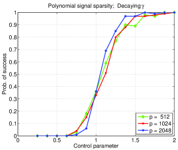
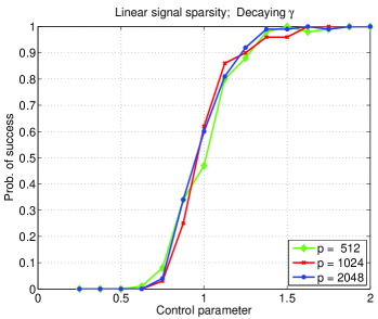
(a)		(b)

Figure 1: Plots of the success probability $\mathbb{P}[\widehat{{S}}={S}]$ versus the control parameter $\theta(n,p,k)=\frac{n}{k\log(p-k)}$ for $\gamma$-sparsified ensembles, with decaying measurement sparsity $\gamma=\frac{{.5\log{(p-k)}}}{\sqrt{p-k}}$. (a) Polynomial signal sparsity $k={\mathcal{O}}(\sqrt{p})$. (b) Linear signal sparsity $k=\Theta(p)$.

5 Discussion

In this paper, we have studied the problem of recovery the support set of a sparse vector $\beta^{*}$ based on noisy observations. The main result is to show that it is possible to “sparsify” standard dense measurement matrices, so that they have a vanishing fraction of non-zeroes per row, while retaining the same sample complexity (number of observations $n$) required for exact recovery. We also showed that under the support recovery metric and in the presence of noise, no method can succeed without the number of non-zeroes per column tending to infinity. See also the paper [22] for complementary results on the information-theoretic scaling of sparse measurement ensembles.

The approach taken in this paper is to find rates which $\gamma$ (as a function of $n$, $p$, $k$) can safely tend towards zero while maintaining the same statistical efficiency as dense random matrices. In various practical settings [21], it may be preferable to make the measurement ensembles even sparser at the cost of taking more measurements $n$ and thus decreasing efficiency relative to dense random matrices. A natural question is the sample complexity $n(\gamma,p,k)$ in this regime as well. Finally, this work has focused only on a randomly sparsified matrices, as opposed to particular sparse designs (e.g., based on LDPC or expander-type constructions [7, 16, 23]). Although our results imply that exact support recovery with noisy observations is impossible with bounded degree designs, it would be interesting to examine the trade-off between other loss functions (e.g, $\ell_{2}$ reconstruction error) and sparse measurement designs.

Acknowledgments

This work was partially supported by NSF grants CAREER-CCF-0545862 and DMS-0605165, a Vodafone-US Foundation Fellowship (DO), and a Sloan Foundation Fellowship (MJW).

Appendix A Standard concentration results

In this appendix, we collect some tail bounds used repeatedly throughout this paper.

Lemma 7 (Hoeffding bound [9]).

Given a binomial variate $Z\sim\operatorname{Bin}(n,\gamma)$, we have for any $\delta>0$

$${\mathbb{P}}{[|Z-\gamma n|\geq\delta n]} \leq 2\,\exp\big{(}-2n\delta^{2}\big{)}.$$

Lemma 8 ($\chi^{2}$-concentration [10]).

Let $X\sim\chi^{2}_{m}$ be a chi-squared variate with $m$ degrees of freedom. Then for all $\frac{1}{2}>\delta\geq 0$, we have

$${\mathbb{P}}{[X-m\geq\delta m]} \leq \exp\left(-\frac{3}{16}m\delta^{2}\right).$$

We will also find the following standard Gaussian tail bound [11] useful:

Lemma 9 (Gaussian tail behavior).

Let $V\sim N(0,\sigma^{2})$ be a zero-mean Gaussian with variance $\sigma^{2}$. Then for all $\delta>0$, we have

$$\mathbb{P}[|V|>\delta] \leq 2\;\exp\big{(}-\frac{\delta^{2}}{2\sigma^{2}}\big{)}.$$

Appendix B Convex optimality conditions

B.1 Proof of Lemma 2

Let $f(\beta):=\frac{1}{2n}\|{{Y}}-X\beta\|_{2}^{2}+\rho_{n}\|\beta\|_{1}$ denote the objective function of the Lasso (4). By standard convex optimality conditions [15], a vector $\widehat{\beta}\in{\mathbb{R}}^{p}$ is a solution to the Lasso if and only if $0\in\mathbb{R}^{p}$ is an element of the subdifferential of $f(\beta)$ at $\widehat{\beta}$. These conditions lead to

$$\frac{1}{n}X^{T}(X\widehat{\beta}-{{Y}})+\rho_{n}\widehat{z} = 0,$$

where the dual vector $\widehat{z}\in{\mathbb{R}}^{p}$ is an element of the subdifferential of the $\ell_{1}$-norm, given by

$$\partial\|\widehat{\beta}\|_{1} = \left\{z\in{\mathbb{R}}^{p}\;\mid\;z_{i}=\operatorname{sign}(\widehat{\beta}_{i})\textrm{ if }\widehat{\beta}_{i}\neq 0,\qquad z_{i}\in[-1,1]\textrm{ otherwise}\right\}.$$

Now suppose that we are given a pair $(\widehat{\beta},\widehat{z})\in{\mathbb{R}}^{p}\times{\mathbb{R}}^{p}$ that satisfy the assumptions of Lemma 2. Condition (12) is equivalent to $(\widehat{\beta},\widehat{z})$ satisfying the zero subgradient condition. Conditions (13a), (13c) and (13d) ensure that $\widehat{z}$ is an element of the subdifferential of the $\ell_{1}$-norm at $\widehat{\beta}$. Finally, conditions (13b) and (13d) ensure that $\widehat{\beta}$ correctly specifies the signed support.

It remains to verify that $\widehat{\beta}$ is the unique optimal solution. By Lagrangian duality, the Lasso problem (4) (given in penalized form) can be written as an equivalent constrained optimization problem over the ball $\|\beta\|_{1}\leq C(\rho_{n})$, for some constant $C(\rho_{n})<+\infty$. Equivalently, we can express this single $\ell_{1}$-constraint as a set of $2^{p}$ linear constraints ${\vec{v}}^{T}\beta\leq C$, one for each sign vector ${\vec{v}}\in\{-1,+1\}^{p}$. The vector $\widehat{z}$ can be written as a convex combination $\widehat{z}=\sum_{{\vec{v}}}\alpha^{*}_{\vec{v}}{\vec{v}}$, where the weights $\alpha^{*}_{\vec{v}}$ are non-negative and sum to one. By construction of $\widehat{\beta}$ and $\widehat{z}$, the weights $\alpha^{*}$ form an optimal Lagrange multiplier vector for the problem. Consequently, any other optimal solution—say $\widetilde{\beta}$—must also minimize the associated Lagrangian

$$L(\beta;\alpha^{*}) = f(\beta)+\sum_{{\vec{v}}}\alpha^{*}_{\vec{v}}\left[{\vec{v}}^{T}\beta-C\right],$$

and satisfy the complementary slackness conditions $\alpha^{*}_{\vec{v}}\left({\vec{v}}^{T}\widetilde{\beta}-C\right)=0$. Note that these complementary slackness conditions imply that $\widehat{z}^{T}\widetilde{\beta}=C$. But this can only happen if $\widetilde{\beta}_{j}=0$ for all indices where $|\widehat{z}_{j}|<1$. Therefore, any optimal solution $\widetilde{\beta}$ satisfies $\widetilde{\beta}_{{S^{c}}}=0$. Finally, given that all optimal solutions satisfy $\beta_{{S^{c}}}=0$, we may consider the restricted optimization problem subject to this set of constraints. If the Hessian submatrix $\widehat{\Sigma}_{{S}{S}}$ is strictly positive definite, then this sub-problem is strictly convex, so that $\widehat{\beta}$ must be the unique optimal solution, as claimed.

B.2 Derivation of $\{V^{a}_{j},V^{b}_{j},U_{i}\}$

In this appendix, we derive the form of the $\{V^{a}_{j},V^{b}_{j}\}$ and $\{U_{i}\}$ variables defined in equations (16a) through (16c). We begin by writing the zero sub-gradient condition in a block-form, and substituting the relations specified in conditions (13a) and (13b):

$$\begin{bmatrix}\widehat{\Sigma}_{{S}{S}}&\widehat{\Sigma}_{{S}{S^{c}}}\\ \widehat{\Sigma}_{{S^{c}}{S}}&\widehat{\Sigma}_{{S^{c}}{S^{c}}}\end{bmatrix}\begin{bmatrix}\widehat{\beta}_{S}-\beta^{*}_{S}\\ 0\end{bmatrix}+\begin{bmatrix}\frac{1}{n}X_{S}^{T}W\\ \frac{1}{n}X_{{S^{c}}}^{T}W\end{bmatrix}+\rho_{n}\begin{bmatrix}\operatorname{sign}(\beta^{*}_{S})\\ \widehat{z}_{{S^{c}}}\end{bmatrix} = 0.$$

By solving the top block, we obtain

$$U:=\widehat{\beta}_{S}-\beta^{*}_{S} = -\widehat{\Sigma}_{{S}{S}}^{-1}\left\{\frac{1}{n}X^{T}_{S}{{W}}+\rho_{n}\operatorname{sign}(\beta^{*}_{S})\right\}.$$

By back-substituting this relation into the lower block, we can solve explicitly for $\widehat{z}_{{S^{c}}}$; doing so yields that $\widehat{z}_{{S^{c}}}=V^{a}+V^{b}$, where the $(p-k)$-vectors are defined in equations (16a) and (16b).

Appendix C Proof of Lemma 6

Let $Z\in{\mathbb{R}}^{n\times n}$ denote a $n\times n$ matrix, for which the off-diagonal elements $Z_{ij}=0$ for all $i\neq j$, and the diagonal elements $Z_{ii}\sim\operatorname{Ber}(\gamma)$ are i.i.d. With this notation, we can write $H\overset{d}{=}Zh$. Using the definition (21) of $h$, we have

$$\|\,H\,\|_{2}^{2} = \|Zh\|_{2}^{2}$$

$$= \|Z\;\frac{X_{S}}{n}(\widehat{\Sigma}_{{S}{S}})^{-1}\vec{1}\|_{2}^{2}$$

$$= \vec{1}^{T}(\widehat{\Sigma}_{{S}{S}})^{-1}(Z\frac{X_{S}}{n})^{T}(Z\frac{X_{S}}{n})(\widehat{\Sigma}_{{S}{S}})^{-1}\vec{1}$$

$$= \frac{\gamma}{n}\vec{1}^{T}(\widehat{\Sigma}_{{S}{S}})^{-1}\underbrace{\left\{\frac{1}{\gamma n}\sum_{i=1}^{n}\mathbb{I\,}[Z_{ii}=1]\;x_{i}x_{i}^{T}\right\}}(\widehat{\Sigma}_{{S}{S}})^{-1}\vec{1}$$

$$\qquad\qquad\qquad\qquad\Gamma(Z)$$

where $x_{i}$ is the $i^{th}$ row of the matrix $X_{S}$. From Lemma 10 with $\theta=1$ and $t=(p-k)$, we have

$$\mathbb{P}\left[|\!|\!|{\widehat{\Sigma}_{{S}{S}}}^{-1}|\!|\!|_{2}\geq f_{1}(p,k,\gamma)\right] \leq \frac{1}{(p-k)^{2}}$$ (27)

where $f_{1}(p,k,\gamma):=\left(1-\mathcal{O}\Big{(}\frac{1}{\gamma}\sqrt{\max\left\{\frac{1}{k},\frac{\log\log(p-k)}{\log(p-k)}\right\}}\Big{)}\right)^{-1}$.

Next we control the spectral norm of the random matrix $\Gamma(Z)$, conditioned on the total number $\sum_{i=1}^{n}Z_{ii}$ of non-zero entries. In particular, applying Lemma 10 with $t=p-k$, and $\theta=1$, we have

$${\mathbb{P}}\left[\|\,\Gamma{Z}\,\|_{2}\geq\frac{z}{n\gamma}\big{[}1+\frac{C}{\frac{z}{n}}\sqrt{\max\left\{\frac{1}{k{\frac{z}{n}}},\frac{\log{\frac{z}{n}}\log(p-k)}{{\frac{z}{n}}\log(p-k)}\right\}}\big{]}\;\mid\;\sum_{i=1}^{n}Z_{ii}=z\right] \leq \frac{1}{(p-k)^{2}},$$ (28)

as long as $k\frac{z}{n}\rightarrow\infty$.

The next step is to deal with the conditioning. Define the event

$$\mathcal{T}(k,\gamma) := \left\{Z\;\mid\;\gamma-\frac{1}{\sqrt{2k}}\leq\frac{1}{n}\sum_{i=1}^{n}Z_{ii}\leq\gamma+\frac{1}{2\sqrt{k}}\right\}.$$

Defining the function

$$f_{2}(p,k,\gamma) := \Biggr{(}1+\frac{1}{2\sqrt{k}\gamma}\Biggr{)}\;\Biggr{[}1+\mathcal{O}\Big{(}\frac{1}{\gamma}\sqrt{\max\left\{\frac{1}{k(\gamma-\frac{1}{2\sqrt{k}})},\frac{\log{(\gamma+\frac{1}{2\sqrt{k}})\log(p-k)}}{(\gamma-\frac{1}{2\sqrt{k}})\log(p-k)}\right\}}\Big{)}\Biggr{]},$$

we have

$$\mathbb{P}[|\!|\!|\Gamma(Z)|\!|\!|_{2}\geq f_{2}(p,k,\gamma)] \leq \mathbb{P}[|\!|\!|\Gamma(Z)|\!|\!|_{2}\geq f_{2}(p,k,\gamma)\;\mid\;\mathcal{T}(k,\gamma)]+\mathbb{P}[(\mathcal{T}(k,\gamma))^{c}]$$ (29)

$$\leq \exp(-{2}\log(p-k))+2\exp(-\frac{n}{2k})$$

$$\leq 3\exp(-\min\{2\log(p-k),\frac{n}{2k}\}),$$

where we have used the bound (28), and the Hoeffding bound (see Lemma 7).

Combining the bounds (27) and (29), we conclude that as long as $\gamma k\rightarrow\infty$, then:

$$\mathbb{P}\left[|\!|\!|\widehat{\Sigma}^{-1}\Gamma(Z)\widehat{\Sigma}^{-1}|\!|\!|_{2}\geq f_{1}^{2}f_{2}\right] \leq 4\exp(-\min\{2\log(p-k),\frac{n}{2k}\}).$$

Since $\|\vec{1}\|_{2}=\sqrt{k}$, we have

$$\mathbb{P}[\|H\|_{2}^{2}\geq\frac{\gamma k}{n}f_{1}^{2}f_{2}] \leq 4\exp(-\min\{2\log(p-k),\frac{n}{2k}\}).$$

To conclude the proof, we note that assumption (8c) implies that both $f_{1}(p,k,\gamma)$ and $f_{2}(p,k,\gamma)$ converge to $1$ as $(p,k,\gamma)$ scale. In particular, for any fixed $\delta>0$, we have $f_{1}^{2}f_{2}<(1+\delta)$ for $(p,k)$ sufficiently large, so that Lemma 6 follows.

Appendix D Singular values of sparsified matrices

Let $\theta(p,k)\in(0,1]$ and $t(p,k)\in\{1,2,3,\ldots\}$ be functions. Let $X$ be an $\theta n\times k$ random matrix with i.i.d. entries $X_{ij}$ distributed according to the $\gamma$-sparsified ensemble (6).

Lemma 10.

Suppose that $n\geq(2+\nu)k\log{(p-k)}$ for some $\nu>0$. If as $k,p-k,\rightarrow\infty$

$$T(\gamma,k,p,\theta,t) := \frac{1}{\gamma}\sqrt{\max\left\{\frac{\log{(t)}}{\theta k\log{(p-k)}},\frac{\log[\theta\log(p-k)]}{\theta\log(p-k)}\right\}}\;\longrightarrow\;0$$

then for some constant $C\in(0,\infty)$, we have

$$\mathbb{P}\left[\sup_{\|u\|_{2}=1}\big{|}\frac{1}{\sqrt{\theta n}}\|Xu\|_{2}-1\big{|}\geq C\,T(\gamma,k,p,\theta,t)\right] \leq \mathcal{O}(\frac{1}{t^{2}}),$$ (30)

Note that Lemma 10 with $\theta=1$ and $t=p-k$ implies that $\widehat{\Sigma}=\frac{1}{n}X_{S}^{T}X_{S}$ is invertible with probability greater than $1-\mathcal{O}(\frac{1}{(p-k)^{2}})$, there establishing Lemma 1. Other settings in which this lemma is applied are $(\theta,t)=(\gamma,p-k)$ and $(\theta,t)=(1,k)$. The remainder of this section is devoted to the proof of Lemma 10.

D.1 Bounds on expected values

Let $X\in{\mathbb{R}}^{{\theta n}\times k}$ be a random matrix with i.i.d. entries, of the sparsified Gaussian form

$$X_{ij} \sim (1-\gamma)\delta_{X}(0)+\gamma N(0,\frac{1}{\gamma}).$$

Note that ${\mathbb{E}}[X_{ij}]=0$ and $\operatorname{var}(X_{ij})=1$ by construction.

We follow the proof technique outlined in [19]. We first note the tail bound:

Lemma 11.

Let $Y_{1},\ldots,Y_{d}$ be i.i.d. samples of the $\gamma$-sparsified ensemble. Given any vector $a\in{\mathbb{R}}^{d}$ and $t>0$, we have $\mathbb{P}[\sum_{i=1}^{d}a_{i}Y_{i}>t]\leq\exp\left(-\frac{\gamma t^{2}}{2\|a\|^{2}_{2}}\right)$.

To establish this bound, note that each $Y_{i}$ is dominated (stochastically) by the random variable $Z\sim N(0,\frac{1}{\gamma})$. In particular, we have

$$\mathbb{M}_{Y_{i}}(\lambda) = {\mathbb{E}}[\exp(\lambda Y_{i})]\;=\;(1-\gamma)+\gamma{\mathbb{E}}[\exp(\lambda Z)]\leq\exp(\lambda^{2}/2\gamma).$$

Now let us bound the maximum singular value $s_{k}(X)$ of the random matrix $X$. Letting $S^{d-1}$ denote the $\ell_{2}$ unit ball in $d$ dimensions, we begin with the variational representation

$$s_{k}(X) = \max_{u\in S^{k-1}}\|Xu\|$$

$$= \max_{v\in S^{{\theta n}-1}}\;\max_{u\in S^{k-1}}v^{T}Xu.$$

For an arbitrary $\epsilon\in(0,1)$, we can find $\epsilon$-covers (in $\ell_{2}$ norm) of $S^{{\theta n}-1}$ and $S^{k-1}$ with $M_{\theta n}(\epsilon)=(3/\epsilon)^{{\theta n}}$ and $M_{k}(\epsilon)=(3/\epsilon)^{k}$ points respectively [12]. Denote these covers by $C_{\theta n}(\epsilon)$ and $C_{k}(\epsilon)$ respectively. A standard argument shows that for all $\epsilon\in(0,1)$, we have

$$\|X\|_{2} \leq \frac{1}{(1-\epsilon)^{2}}\max_{u_{\alpha}\in C_{k}(\epsilon)}\;\max_{v_{\beta}\in C_{\theta n}(\epsilon)}v_{\beta}^{T}Xu_{\alpha}.$$

Let us analyze the maximum on the RHS: for a fixed pair $(u,v)$ in our covers, we have

$$u^{T}Xv = \sum_{i=1}^{\theta n}\sum_{j=1}^{k}X_{ij}u_{i}v_{j}.$$

Let us apply Lemma 11 with $d={\theta n}k$, and weights $a_{ij}=u_{i}v_{j}$. Note that we have

$$\|a\|^{2}_{2}= = \sum_{i,j}a_{ij}^{2}\;=\;\sum_{i}u_{i}^{2}(\sum_{j}v_{j}^{2})\;=\;1$$

since each $u$ and $v$ are unit norm. Consequently, for any fixed $u,v$ in the covers, we have

$$\mathbb{P}[u^{T}Xv>t] \leq \exp\left(-\frac{\gamma t^{2}}{2}\right)$$

By the union bound, we have

$$\mathbb{P}\left[\max_{u_{\alpha}\in C_{k}(\epsilon)}\;\max_{v_{\beta}\in C_{\theta n}(\epsilon)}v_{\beta}^{T}Xu_{\alpha}>t\right] \leq M_{k}(\epsilon)M_{\theta n}(\epsilon)\exp\left(-\frac{\gamma t^{2}}{2}\right)$$

$$\leq \exp\left((k+{\theta n})\log(3/\epsilon)-\frac{\gamma t^{2}}{2}\right).$$

By choosing $\epsilon=\frac{1}{2}$ and $t=\sqrt{\frac{4}{\gamma}(k+{\theta n})\log 6}$, we can conclude that

$$s_{1}(X)/\sqrt{{\theta n}}\;=\;\|X\|_{2}/\sqrt{{\theta n}} \leq C\sqrt{\frac{1}{\gamma}}\;\sqrt{1+\frac{k}{{\theta n}}}$$

w.p. $1-\exp(-(k+{\theta n})\log 6)$. Note that

$$\frac{k}{\theta n} = \mathcal{O}\left(\frac{1}{(2+\nu)\theta\log(p-k)}\right)\rightarrow 0,$$

since $\frac{\log[\theta\log(p-k)]}{\theta\log{(p-k)}}\rightarrow 0$, which implies that $\theta\log{(p-k)}\rightarrow\infty$.

Consequently, we can conclude that

$$\|X\|_{2}/\sqrt{{\theta n}} \leq \mathcal{O}(1/\sqrt{\gamma})$$

w.p. one as ${\theta n},k\rightarrow\infty$. Although this bound is essentially correct for a $\mathcal{N}(0,\frac{1}{\gamma})$ ensemble with $\gamma$ fixed, it is very crude for the sparsified case with $\gamma\rightarrow 0$, but will useful in obtaining tighter control on $s_{1}(X)$ and $s_{k}(X)$ in the sequel.

D.2 Tightening the bound

For a given $u\in S^{k-1}$, consider the random variable $\|Xu\|_{2}^{2}:=\sum_{i=1}^{\theta n}(Xu)^{2}_{i}$. We first claim that each variate $Z_{i}=(Xu)_{i}^{2}$ is subexponential:

Lemma 12.

For any $t>0$, we have $\mathbb{P}[Z_{i}>t]\leq 2\exp\left(-\frac{\gamma t}{2}\right)$.

Proof.

We can write $(Xu)_{i}=\sum_{j=1}^{k}X_{ij}u_{j}$ where $\|u\|_{2}=1$. Hence, from Lemma 11, we have

$$\mathbb{P}[\sum_{j=1}^{k}X_{ij}u_{j}>\delta] \leq \exp(-\frac{\gamma\delta^{2}}{2}).$$

By symmetry, we have $\mathbb{P}[Z_{i}>t]=\mathbb{P}[|\sum_{j=1}^{k}X_{ij}u_{j}|>\sqrt{t}]\;\leq\;2\exp(-\frac{\gamma t}{2})$ as claimed. ∎

Now consider the event

$$\mathbb{P}\left[\left|\frac{\|Xu\|^{2}_{2}}{{\theta n}}-1\right|>\delta\right] = \mathbb{P}\left[\left|\sum_{i=1}^{\theta n}Z_{i}-{\mathbb{E}}[\sum_{i=1}^{\theta n}Z_{i}]\right|>\delta{\theta n}\right]$$

We may apply Theorem 1.4 of Vershynin [19] with $b=8{\theta n}/\gamma^{2}$ and $d=2/\gamma$. Hence, we have $4b/d=16{\theta n}/\gamma$, which grows at least linearly in ${\theta n}$. Hence, for any $\delta>0$ less than $16{\theta n}/\gamma$ (we will in fact take $\delta\rightarrow 0$), we have

$$\mathbb{P}\left[\left|\frac{\|Xu\|^{2}_{2}}{{\theta n}}-1\right|>\delta\right] \leq 2\exp\left(-\frac{\delta^{2}{(\theta n)}^{2}}{256{\theta n}/\gamma^{2}}\right)\;=\;2\exp\left(-\frac{\gamma^{2}\;\delta^{2}{\theta n}}{256}\right).$$

Now take an $\epsilon$-cover of the $k$-dimensional $\ell_{2}$ ball, say with $N(\epsilon)\;=\;(3/\epsilon)^{k}$ elements. By union bound, we have

$$\mathbb{P}\left[\inf_{i=1,\ldots,N(\epsilon)}\frac{\|Xu_{i}\|^{2}_{2}}{{\theta n}}<1-\delta\right] \leq \exp\left(-\frac{\gamma^{2}\;\delta^{2}{\theta n}}{256}+k\log(3/\epsilon)\right)$$

Now set

$$\delta=\frac{\sqrt{2}}{\gamma}\sqrt{\frac{256f(k,p)k\log(3/\epsilon)}{{\theta n}}},$$

where $f(k,p)\geq 1$ is a function to be specified. Doing so yields that the infimum is bounded by $1+\delta$ with probability $1-\exp(-kf(k,p)\log(3/\epsilon))$. (Note that the choice of $f(k,p)$ influences the rate of convergence, hence its utility.)

For any element $u\in S^{k-1}$, we have some $u_{i}$ in the cover, and moreover

$$\left|\|Xu\|^{2}-\|Xu_{i}\|^{2}\right| = \left|\left\{\|Xu\|-\|Xu_{i}\|\right\}\;\left\{\|Xu\|+\|Xu_{i}\|\right\}\right|$$

$$\leq \;\left|\left\{\|Xu\|-\|Xu_{i}\|\right\}\right|\;(2\|X\|)\;\;$$

$$\leq (\|X\|\;\|u-u_{i}\|)\;\;(2\|X\|)\;\leq\;2\|X\|^{2}\epsilon$$

From our earlier result, we know that $\|X\|^{2}=\mathcal{O}({\theta n}/\gamma)$ with probability $1-\exp(\log{6}(k+{\theta n}))$. Putting together the pieces, we have that the bound

$$\frac{1}{{\theta n}}\inf_{u\in S^{k-1}}\|Xu\|^{2} \geq 1+\delta+C_{2}\epsilon/\gamma\;=\;1+\frac{2}{\gamma}\sqrt{\frac{32f(k,p)k\log(3/\epsilon)}{{\theta n}}}+\frac{C_{2}}{\gamma}\epsilon,$$

for some constant $C_{2}>0$ independent of ${\theta n},k,\gamma$, holds with probability at least

$$\min\{1-\exp(-kf(k,p)\log(3/\epsilon)),1-\exp(-\log{6}(k+{\theta n}))\},$$ (31)

Now set $\epsilon=3k/{\theta n}$, so that we have w.h.p.

$$\frac{1}{{\theta n}}\inf_{u\in S^{k-1}}\|Xu\|^{2} \geq 1-\frac{C_{3}}{\gamma}\sqrt{f(k,p)\frac{k}{{\theta n}}\log(\frac{{\theta n}}{k})}$$

(Note that we have utilized the fact that both $\sqrt{f(k,p)\frac{k}{{\theta n}}\log(\frac{{\theta n}}{k})}$ and $\frac{k}{{\theta n}}\rightarrow 0$, but the former more slowly than the latter.)

Since $k/{\theta n}\rightarrow 0$, this quantity will go to zero, as long as $f(k,p)$ remains fixed, or scales slowly enough. To understand how to choose $f(k,p)$, let us consider the rate of convergence (31). To establish the claim (30), we need rates fast enough to dominate a $\log(t)$ term in the exponent, which guides our choice of $f(k,p)$. Recall that we are seeking to prove a scaling of the form ${n}=\Theta(k\log(p-k))$, so that our requirement (with $\epsilon=3k/{\theta n}=\frac{3}{\theta\log(p-k)}$) is equivalent to the quantity

$$kf(k,p)\log(3/\epsilon)-\log(t) = kf(k,p)\log[\theta\log(p-k)]-\log(t)$$

tending to infinity. First, if $k>\frac{\log(t)}{\log[\theta\log(p-k)]}$, then we may simply set $f(k,p)=2$. Otherwise, if $k\leq\frac{\log(t)}{\log\theta\log(p-k)}$, then we may set

$$f(k,p)=2\frac{\log(t)}{k\log\theta\log(p-k)}\geq 1.$$

If $f(k,p)=2$, then we have

$$f(k,p)\frac{k}{{\theta n}}\log(\frac{{\theta n}}{k}) = 2\frac{\log[\theta\log(p-k)]}{\theta\log(p-k)}\;\rightarrow\;0.$$

In the other case, if $k\leq\frac{\log(t)}{\log\theta\log(p-k)}$, we have

$$f(k,p)\frac{k}{{\theta n}}\log(\frac{{\theta n}}{k}) \leq 2\frac{\log(t)}{k\log\theta\log(p-k)}\frac{1}{\theta\log(p-k)}\log\theta\log(p-k)\;=\;\frac{2}{k}\frac{\log{t}}{\theta\log{(p-k)}}\rightarrow 0,$$

which again follows from the assumptions in Lemma 10.

Recalling the definition of $T(\gamma,k,p,\theta,t)$ from Lemma 10, we can summarize both cases can be summarized cleanly by saying that with probability greater than $1-\frac{1}{t^{2}}$:

$$\frac{1}{{\theta n}}\inf_{u\in S^{k-1}}\|Xu\|^{2} \geq 1-\frac{C}{\gamma}\sqrt{\max\left\{\frac{1}{k}\frac{\log{t}}{\theta\log{(p-k)}},\frac{\log\theta\log(p-k)}{\theta\log(p-k)}\right\}}$$

$$= 1-CT(\gamma,k,p,\theta,t)$$

Because $T(\gamma,k,p,\theta,t)\rightarrow 0$, for all $p\geq p_{1}^{*}$, $k\geq k_{1}^{*}$, $CT(\gamma,k,p,\theta,t)<1$. Thus we can take square root of both sides and apply the identity $\sqrt{1+x}=1+\frac{x}{2}+o(x)$ (valid for $|x|<1$) to conclude that, with probability greater than $1-\frac{C_{1}(p_{1}^{*},k_{1}^{*})}{t^{2}}$:

$$\frac{1}{\sqrt{{\theta n}}}\inf_{u\in S^{k-1}}\|Xu\| \geq 1-\frac{C}{2}T(\gamma,k,p,\theta,t)+o(T(\gamma,k,p,\theta,t)),$$

As $T(\gamma,k,p,\theta,t)\rightarrow 0$, for all $k\geq k_{2}^{*}$, $p\geq p_{2}^{*}$ we have that $|o(T(\gamma,k,p,\theta,t))|<\frac{C}{4}T(\gamma,k,p,\theta,t)$

Thus, with probability greater than $1-\frac{C_{2}(p_{1}^{*},k_{1}^{*},p_{2}^{*},k_{2}^{*})}{t^{2}}$:

$$\frac{1}{\sqrt{{\theta n}}}\inf_{u\in S^{k-1}}\|Xu\| \geq 1-\frac{3C}{4}T(\gamma,k,p,\theta,t),$$

Note that this same process can be repeated to bound the maximum singular value, yielding the following result:

$$\frac{1}{\sqrt{{\theta n}}}\sup_{u\in S^{k-1}}\|Xu\| \leq 1+\frac{3C}{4}T(\gamma,k,p,\theta,t),$$

Combining these two bounds, we have proved Lemma 10.

References

• [1] S. Boyd and L. Vandenberghe. Convex optimization. Cambridge University Press, Cambridge, UK, 2004.
• [2] E. Candes and T. Tao. Decoding by linear programming. IEEE Trans. Info Theory, 51(12):4203–4215, December 2005.
• [3] S. Chen, D. L. Donoho, and M. A. Saunders. Atomic decomposition by basis pursuit. SIAM J. Sci. Computing, 20(1):33–61, 1998.
• [4] G. Commode and S. Muthukrishnan. Towards an algorithmic theory of compressed sensing. Technical report, Rutgers University, July 2005.
• [5] D. Donoho. For most large underdetermined systems of linear equations, the minimal $\ell_{1}$-norm near-solution approximates the sparsest near-solution. Communications on Pure and Applied Mathematics, 59(7):907–934, July 2006.
• [6] D. Donoho. For most large underdetermined systems of linear equations, the minimal $\ell_{1}$-norm solution is also the sparsest solution. Communications on Pure and Applied Mathematics, 59(6):797–829, June 2006.
• [7] J. Feldman, T. Malkin, R. A. Servedio, C. Stein, and M. J. Wainwright. LP decoding corrects a constant fraction of errors. IEEE Trans. Information Theory, 53(1):82–89, January 2007.
• [8] A. Gilbert, M. Strauss, J. Tropp, and R. Vershynin. Algorithmic linear dimension reduction in the $\ell_{1}$-norm for sparse vectors. In Proc. Allerton Conference on Communication, Control and Computing, Allerton, IL, September 2006.
• [9] W. Hoeffding. Probability inequalities for sums of bounded random variables. Journal of the American Statistical Association, 58:13–30, 1963.
• [10] I. Johnstone. Chi-square oracle inequalities. In M. de Gunst, C. Klaassen, and A. van der Vaart, editors, State of the Art in Probability and Statistics, number 37 in IMS Lecture Notes, pages 399–418. Institute of Mathematical Statistics, 2001.
• [11] M. Ledoux and M. Talagrand. Probability in Banach Spaces: Isoperimetry and Processes. Springer-Verlag, New York, NY, 1991.
• [12] J. Matousek. Lectures on discrete geometry. Springer-Verlag, New York, 2002.
• [13] N. Meinshausen and P. Buhlmann. High-dimensional graphs and variable selection with the lasso. Annals of Statistics, 2006. To appear.
• [14] P. Ravikumar, M. J. Wainwright, and J. Lafferty. High-dimensional graph selection using $\ell_{1}$-regularized logistic regression. Technical Report 750, UC Berkeley, Department of Statistics, April 2008. Posted at http://arXiv.org/abs/0804.4202; Conference version appeared at NIPS Conference, December 2006.
• [15] G. Rockafellar. Convex Analysis. Princeton University Press, Princeton, 1970.
• [16] S. Sarvotham, D. Baron, and R. G. Baraniuk. Sudocodes: Fast measurement and reconstruction of sparse signals. In Int. Symposium on Information Theory, Seattle, WA, July 2006.
• [17] R. Tibshirani. Regression shrinkage and selection via the lasso. Journal of the Royal Statistical Society, Series B, 58(1):267–288, 1996.
• [18] J. Tropp. Just relax: Convex programming methods for identifying sparse signals in noise. IEEE Trans. Info Theory, 52(3):1030–1051, March 2006.
• [19] R. Vershynin. On large random almost euclidean bases. Acta. Math. Univ. Comenianae, LXIX:137–144, 2000.
• [20] M. J. Wainwright. Sharp thresholds for high-dimensional and noisy recovery of sparsity using using $\ell_{1}$-constrained quadratic programs. Technical Report 709, Department of Statistics, UC Berkeley, 2006.
• [21] M. B. Wakin, J. N. Laska, M. F. Duarte, D. Baron, S. Sarvotham, D. Takhar, K. F. Kelly, and R. G. Baraniuk. An architecture for compressive imaging. IEEE Int. Conf. Image Proc., pages 1273–1276, 8-11 Oct. 2006.
• [22] W. Wang, M. J. Wainwright, and K. Ramchandran. Information-theoretic limits on sparse support recovery: Dense versus sparse measurements. Technical report, Department of Statistics, UC Berkeley, April 2008. Short version presented at Int. Symp. Info. Theory, July 2008.
• [23] W. Xu and B. Hassibi. Efficient compressive sensing with deterministic guarantees using expander graphs. Information Theory Workshop, 2007. ITW ’07. IEEE, pages 414–419, 2-6 Sept. 2007.