[0805.3079] A note on the ABC-PRC algorithm of Sissons et al.(2007)

1 The ABC-PRC Algorithm

A sequential Monte Carlo method for performing approximate Bayesian Computation (“Monte Carlo without likelihoods”) has been proposed by Sissons, Fan and Tanaka (PNAS, 2007). The main algorithm that is used in their paper is given here in Figure 1.

Refer to caption — Figure 1: The ABC-PRC algorithm of Sissons *et al.*, PNAS, 2007

In this algorithm $N$ is the number of particles $\theta$ is a vector of parameters, the $\epsilon_{t}$ are tolerances such that if $\rho(S(x),S(x_{0}))\leq\epsilon$ the simulated summary statistics, $S(x)$ are considered ‘near enough’ to the target summary statistics $S(x_{0})$ , where $\rho()$ is some distance function. The authors state

Samples $\{\theta_{T}^{(i)}\}$ are weighted samples from the posterior distribution $f(\theta|\rho(S(x),X(x_{0}))\leq\epsilon)$ .

They also state

Finally we note that if $K_{t}(\theta_{t}|\theta_{t-1})=L_{t-1}(\theta_{t-1}|\theta_{t})$ , $\mu_{1}(\theta)=\pi(\theta)$ and the prior $\pi(\theta)\propto 1$ over $\Theta$ , then all weights are equal throughout the sampling process and maybe safely ignored…

2 Problematic Aspects

Intuitively the simplified algorithm, which arises from making the assumptions in the latter statement above, is rather puzzling because it is unclear what corrects for the fact that one is sampling from a distribution that, if the transition kernel variance, $K_{t}(\theta_{t}|\theta_{t-1})$ , is small, is progressively moving away from the prior.

In the algorithm given in Figure 1 there is the statement: if $\rho(S(x**),S(x_{0}))\geq\epsilon_{i}$ , then go to PRC2.1. Intuitively this makes the algorithm superficially appear as $N$ parallel MCMC-ABC chains, with the exception that there is resampling among the chains at each iteration. Certainly if one takes the special case of $N=1$ then it looks similar to the ABC-MCMC algorithm of Marjoram et al. (2003). However a crucial difference is that in the ABC-MCMC the current value is the old value if the update is not accepted, otherwise it is the new value, whereas in this SMC algorithm you keep going until you get an acceptance. So in the ABC-MCMC algorithm, you are guaranteed that if the point you update is already from the posterior distribution, the next point will also be from the posterior (as given by the proof, based on satisfying detailed balance, in Marjoram et al, 2003, page 15325), whereas in the SMC this is not the case. To see this, imagine that the kernel chosen has a very small variance (close to 0, in fact). In the ABC-MCMC, following the proof of detailed balance in Marjoram et al (2003), we are guaranteed that if $\theta_{i}$ is drawn from the posterior, then $\theta_{i+1}$ is also drawn from the posterior (whatever variance of the kernel is chosen). In the SMC, for example, imagine that one has only two resampling steps, and imagine that a sample is taken with $\epsilon$ close to 0, and kernel variance close to 0. The first step gives you (almost) the posterior distribution , $\theta_{i}\tilde{p}(\theta|x=x_{c})$ . The next step, since the prior is now actually the posterior, is exactly like performing standard rejection with such a prior, and gives you (almost) $[p(\theta|x=x_{0})]^{2})$ , the square of the posterior distribution, and so on, progressively. Thus, initially at least, the posterior distribution generated at the $i$ th step is an increasingly poor estimate of $[p(\theta|x)]^{i})$ .

3 Examples

As a toy example consider the case of computing the posterior distribution of the parametric mean, $\mu$ of a Gaussian distribution with a known variance $\sigma^{2}$ , given a vector of $n$ observations $y$ . The prior for $\mu$ is taken to be Gaussian with mean $\mu_{0}$ and variance $\tau^{2}$ . The posterior $p(\mu|y)$ is then given as

N\left(\frac{\frac{\mu_{0}}{\tau^{2}}+\frac{n*\bar{y}}{\sigma^{2}}}{\frac{1}{\tau^{2}}+\frac{n}{\sigma^{2}}},\frac{1}{\frac{1}{\tau^{2}}+\frac{n}{\sigma^{2}}}\right),

where $\bar{y}$ is the arithmetic mean of the elements of $y$ , is a sufficient statistic for this problem, and is used as the only statistic for the ABC analyses described here. In order to test the simplified version of the ABC-PRC algorithm above (although the argument applies also to the more complicated version), I let $\tau^{2}\rightarrow\infty$ so that a flat improper prior is assumed, in which case one obtains

N\left(\bar{y},\frac{\sigma^{2}}{n}\right).

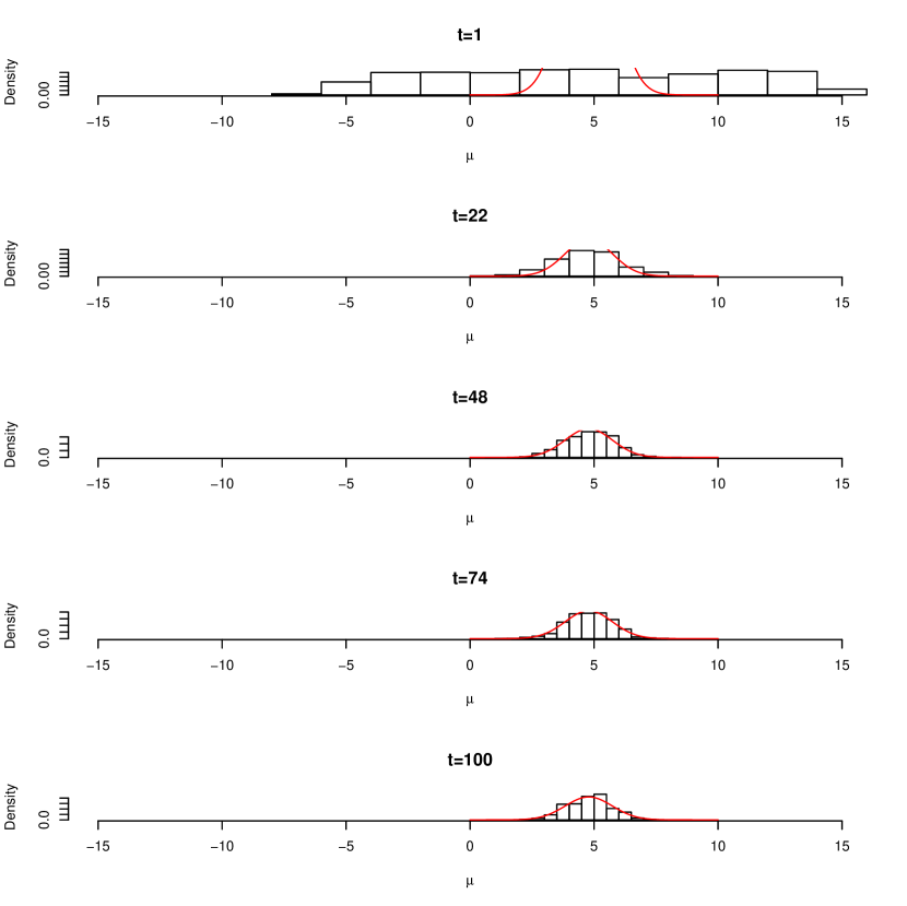
Figure 2 indicates the application of the ABC-PRC algorithm of Sissons et al. (2007) to data with $\bar{y}=4.786624$ and $n=10$ . The known variance, $\sigma^{2}$ is set at 9, and so the posterior variance should be 0.9, with posterior mean of 4.786624. To approximate a flat uniform prior, a uniform with bounds (-15,15) is used for the initial sample.

The ABC-PRC algorithm was run for 100 iterations. The schedule of tolerances is given below:

$t$	$\epsilon_{t}$
1–10	10.0
11–20	5.0
21–30	2.0
31–40	1.0
41–50	0.5
51–60	0.2
61–70	0.1
71–80	0.05
81–90	0.02
91–100	0.01.

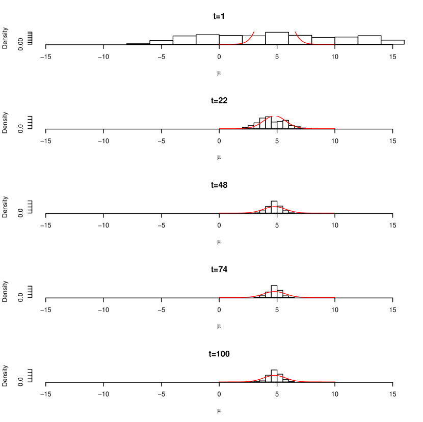
The method converges smoothly, as indicated in Figure 3, but to a variance that is too small. The true posterior variance is 0.9. The posterior variance to which the ABC-PRC method appears to converge is around 0.26.

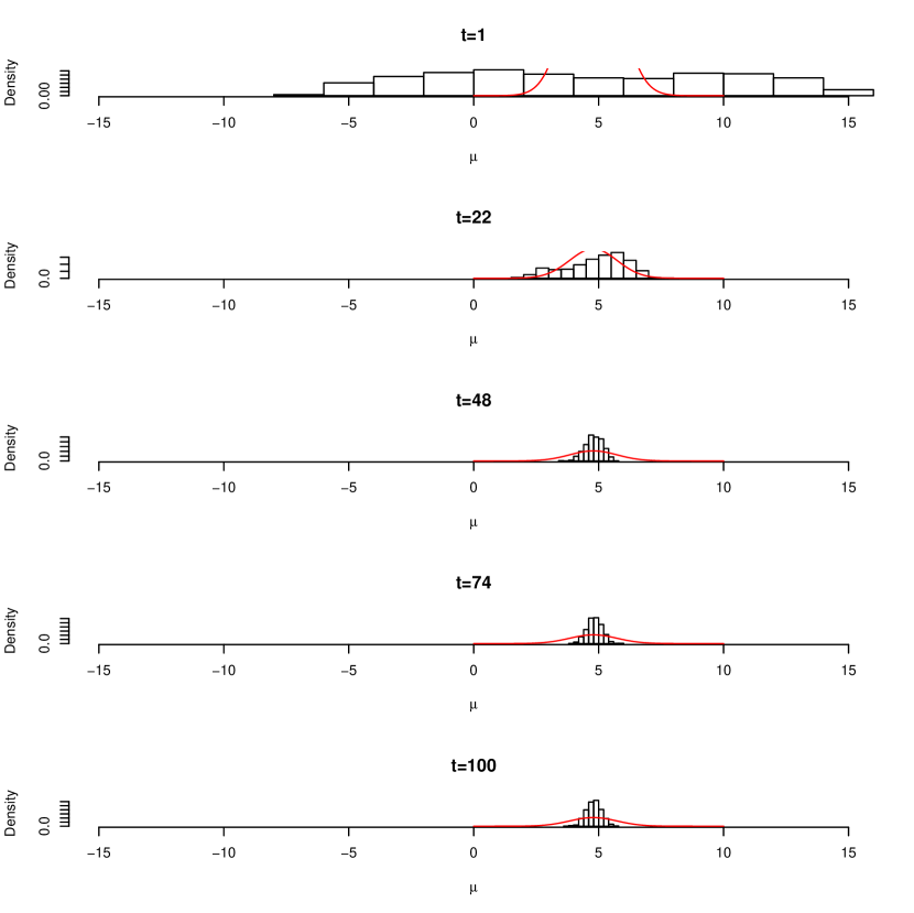
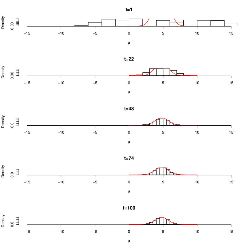
Using an even narrower kernel of 0.01, we can see even greater discrepancies, as illustrated in Figures 4 and 5. In this case the posterior variance to which the method converges is around 0.094, almost one-tenth of the correct value.

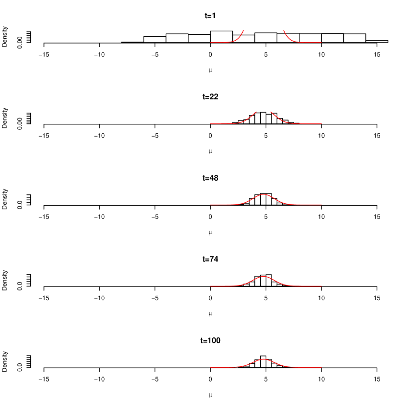
Increasing the variance of the kernel to 1, we see that the estimated posterior variance, now around 0.59, becomes closer to the true value of 0.9 (Figure 7), and, superficially, the posterior distribution looks similar to the theoretical distribution (Figure 6.

Finally with the variance of the kernel at 10, the estimated posterior variance is around 0.84 (Figure 9), still lower than the theoretical value, and the posterior distribution appears very similar to the theoretical distribution (Figure 8).

4 Solution

These results suggest that a good way to look at the ABC-PRC algorithm of Sisson et al. (2007) is as a successive series of applications of the rejection algorithm to random variables drawn from a prior distribution that is a convolution of the smoothing kerneal and the realized variables from the previous rejection round. If this kernel is large relative to the posterior distribution the method will appear to work because it is similar to drawing the variables from a uniform prior. However it can be seen that with a lower kernel variance, the posterior distribution is badly estimated. Viewed in this way, it is clear that the weights do matter, and the appropriate correction, at least for the Gaussian kernel used here, is to compute the weights, $W_{(t),i}$ for the $i$ th particle, from the reciprocal of the (unnormalised) kernel density estimate as

W_{(t),i}=\frac{1}{\sum_{j=0}^{N}p(\theta_{(t),i}|\theta_{(t-1),j},\xi^{2})}

where $p(\theta_{(t),i}|\theta_{(t-1),j},\xi^{2})$ is a Gaussian with mean $\theta_{(t-1),j}$ and variance of the kernel that is used, $\xi^{2}$ .

Figures 10 and 11 show the results of applying this corrected version of the ABC-PRC algorithm to the example with a kernel of variance 0.01, illustrated in Figures 4 and 5. In this case the estimate variance converges to around 0.88, which compares favourably with the uncorrected ABC-PRC algorithm even when a large kernel is used.

In conclusion, it would appear that the ABC-PRC algorithm of Sissons et al. is wrong and should not be used. It can, however, be corrected by the addition of a computationally trivial weighting scheme.

5 Appendix

The R Function for performing the original ABC-PRC

abc.smc1a <- function(npart,niter,unif.lo,unif.hi,y,sigma2,eps,kern.mean,kern.var)
{
# npart is the number of particles
# niter is the number of smc iterations
# unif.lo is the lower limit of the uniform distribution
# unif.hi is the upper limit of the uniform distribution
# y is the real data - we compute the only summary stat - the sample mean - from this
# sigma2 is the known variance.
# eps is the vector of tolerances - the euclidean distance must be less than this

    if(length(eps) != niter)stop("eps is wrong length")
    if(niter < 20)nscore <- niter
    else nscore <- 20
    p.history <- matrix(nrow=nscore,ncol=npart)
    pt <- round(seq(1,niter,length=nscore))
    nsamp <- length(y)
    ymean <- mean(y)
    v1 <- runif(npart,unif.lo,unif.hi)
    k <- 1
    for(j in 1:niter){
        vx <- numeric(0)
        while(T){
            vv <- sample(v1,100*npart,replace=T)
            ssvec <- lapply(lapply(vv,rnorm,n=nsamp,sd=sqrt(sigma2)),mean)
            ind <- sqrt((as.numeric(ssvec) - ymean)^2) <= eps[j]
            if(sum(ind) == 0)next;
            vx <- c(vx,vv[ind])
            if(length(vx) >= npart){
                vx <- vx[1:npart]
                break;
            }
        }
        if(pt[k] == j){
            p.history[k,] <- vx;
            k <- k+1
        }
        v1 <- vx + rnorm(npart,kern.mean,sqrt(kern.var))
    }
    p.history
}

The R function for performing the corrected ABC-PRC

abc.smc1a.correct <- function(npart,niter,unif.lo,unif.hi,y,sigma2,eps,kern.mean,kern.var)
{
# npart is the number of particles
# niter is the number of smc iterations
# unif.lo is the lower limit of the uniform distribution
# unif.hi is the upper limit of the uniform distribution
# y is the real data - we compute the only summary stat - the sample mean - from this
# sigma2 is the known variance.
# eps is the vector of tolerance - the euclidean distance must be less than this

    if(length(eps) != niter)stop("eps is wrong length")
    if(niter < 20)nscore <- niter
    else nscore <- 20
    p.history <- matrix(nrow=nscore,ncol=npart)
    pt <- round(seq(1,niter,length=nscore))
    nsamp <- length(y)
    ymean <- mean(y)
    v1 <- runif(npart,unif.lo,unif.hi)
    wtvec <- rep(1,npart)
    k <- 1
    for(j in 1:niter){
        vx <- numeric(0)
        while(T){
            vv <- sample(v1,100*npart,replace=T,prob=wtvec)
            ssvec <- lapply(lapply(vv,rnorm,n=nsamp,sd=sqrt(sigma2)),mean)
            ind <- sqrt((as.numeric(ssvec) - ymean)^2) <= eps[j]
            if(sum(ind) == 0)next;
            vx <- c(vx,vv[ind])
            if(length(vx) >= npart){
                vx <- vx[1:npart]
                break;
            }
        }
        if(pt[k] == j){
            p.history[k,] <- vx;
            k <- k+1
        }
        v1 <- vx + rnorm(npart,kern.mean,sqrt(kern.var))
       for(jj in 1: npart)wtvec[jj] <- 1.0/sum(dnorm(v1[jj],vx,sqrt(kern.var)))
    }
    p.history
}