Effect of anisotropy on the ground-state magnetic ordering of the
spin-half quantum $J_{1}^{XXZ}$–$J_{2}^{XXZ}$ model on the square lattice

Abstract

We study the zero-temperature phase diagram of the 2D quantum $J_{1}^{XXZ}$–$J_{2}^{XXZ}$ spin-$1/2$ anisotropic Heisenberg model on the square lattice. In particular, the effects of the anisotropy $\Delta$ on the $z$-aligned Néel and (collinear) stripe states, as well as on the $xy$-planar-aligned Néel and collinear stripe states, are examined. All four of these quasiclassical states are chosen in turn as model states on top of which we systematically include the quantum correlations using a coupled cluster method analysis carried out to very high orders. We find strong evidence for two quantum triple points (QTP’s) at ($\Delta^{c}=-0.10\pm 0.15,J_{2}^{c}/J_{1}=0.505\pm 0.015$) and ($\Delta^{c}=2.05\pm 0.15,J_{2}^{c}/J_{1}=0.530\pm 0.015$), between which an intermediate magnetically-disordered phase emerges to separate the quasiclassical Néel and stripe collinear phases. Above the upper QTP ($\Delta\gtrsim 2.0$) we find a direct first-order phase transition between the Néel and stripe phases, exactly as for the classical case. The $z$-aligned and $xy$-planar-aligned phases meet precisely at $\Delta=1$, also as for the classical case. For all values of the anisotropy parameter between those of the two QTP’s there exists a narrow range of values of $J_{2}/J_{1}$, $\alpha^{c_{1}}(\Delta)<J_{2}/J_{1}<\alpha^{c_{2}}(\Delta)$, centered near the point of maximum classical frustration, $J_{2}/J_{1}=\frac{1}{2}$, for which the intermediate phase exists. This range is widest precisely at the isotropic point, $\Delta=1$, where $\alpha^{c_{1}}(1)=0.44\pm 0.01$ and $\alpha^{c_{2}}(1)=0.59\pm 0.01$. The two QTP’s are characterized by values $\Delta=\Delta^{c}$ at which $\alpha^{c_{1}}(\Delta^{c})=\alpha^{c_{2}}(\Delta^{c})$.

I Introduction

The exchange interactions that lead to collective magnetic behavior are clearly of purely quantum-mechanical origin. Nevertheless, the underlying quantum nature has often safely been ignored in describing, at least at the qualitative level, many magnetic phenomena of interest in the past. On the other hand, the investigation of magnetic systems and magnetic phenomena where the intrinsically quantal effects play a dominant role, and hence have to be accounted for in detail, has evolved in recent years to become a burgeoning area at the forefront of condensed matter theory. Thus, the investigation of quantum magnets and their phase transitions, both quantum and thermal, has developed into an extremely active area of research.

From the experimental viewpoint major impetus has come both from the discovery of high-temperature superconductors and, since then, from the ever-increasing ability of materials scientists to fabricate a by now bewildering array of novel magnetic systems of reduced dimensionality, which display interesting quantum phenomena.Scholl:2004 While high-temperature superconductivity has raised the question of the link between the mechanism of superconductivity in the cuprates, for example, and spin fluctuations and magnetic order in one-dimensional (1D) and two-dimensional (2D) spin-half antiferromagnets, the new magnetic materials exhibit a wealth of new quantum phenomena of enormous interest in their own right.

For example, in 1D systems, the universal paradigm of Tomonaga-Luttinger liquid To:1950 ; Lu:1963 behavior has occupied a key position of interest, since Fermi liquid theory breaks down in 1D. More generally, in all restricted geometries the interplay between reduced dimensionality, competing interactions and strong quantum fluctuations, generates a plethora of new states of condensed matter beyond the usual states of quasiclassical long-range order (LRO). Thus, for high-temperature superconductivity, for example, it is suggestedAnd:1987 that quantum spin fluctuation and frustration due to doping could lead to the collapse of the 2D Néel-ordered antiferromagnetic phase present at zero doping, and that this could be the clue for the superconducting behavior. This, and many similar experimental observations for other magnetic materials of reduced dimensionality, has intensified the study of order-disorder quantum phase transitions. Thus, low-dimensional quantum antiferromagnets have attracted much recent attention as model systems in which strong quantum fluctuations might be able to destroy magnetic LRO in the ground state (GS). In the present paper we consider a system of $N\rightarrow\infty$ spin-1/2 particles on a spatially isotropic 2D square lattice.

The spin-1/2 Heisenberg antiferromagnet with only nearest-neighbor (NN) bonds, all of equal strength, exhibits magnetic LRO at zero temperature on such bipartite lattices as the square lattice considered here. A key mechanism that can then destroy the LRO for such systems, with a given lattice and spins of a given spin quantum number $s$, is the introduction of competing or frustrating bonds on top of the NN bonds. The interested reader is referred to Refs. [Scholl:2004, ; Ma:1991, ] for a more detailed discussion of 2D spin systems in general.

An archetypal model of the above type that has attracted much theoretical attention in recent years (see, e.g., Refs. [Ch:1988, ; Dag:1989, ; Ch:1990, ; Schulz:1992, ; Ri:1993, ; Ig:1993, ; Bi:1998_PRB58, ; Ca:2000, ; Ca:2001, ; Siu:2001, ; Su:2001, ; Be:2002, ; Sin:2003, ; Zhang:2003, ]) is the 2D spin-1/2 $J_{1}$–$J_{2}$ model on a square lattice with both NN and next-nearest-neighbor (NNN) antiferromagnetic interactions, with strength $J_{1}>0$ and $J_{2}>0$ respectively. The NN bonds $J_{1}>0$ promote Néel antiferromagnetic order, while the NNN bonds $J_{2}>0$ act to frustrate or compete with this order. All such frustrated quantum magnets continue to be of great theoretical interest because of the possible spin-liquid and other such novel magnetically disordered phases that they can exhibit (and see, e.g., Ref. [Mi:2005, ]). The recent syntheses of magnetic materials that can be well described by the spin-1/2 $J_{1}$–$J_{2}$ model on the 2D square lattice, such as the undoped precursors to the high-temperature superconducting cuprates for small $J_{2}/J_{1}$ values, VOMoO₄ for intermediate $J_{2}/J_{1}$ values,Car:2002 and Li₂VOSiO₄ for large $J_{2}/J_{1}$ values,Mel:2000 ; Ro:2002 has fuelled further theoretical interest in the model.

The properties of the spin-1/2 $J_{1}$–$J_{2}$ model on the 2D square lattice are well understood in the limits when $J_{2}=0$ or $J_{1}=0$. For the case when $J_{2}=0$, and the classical GS is perfectly Néel-ordered, the quantum fluctuations are not sufficiently strong enough to destroy the Néel LRO, although the staggered magnetization is reduced to about 61% of its classical value. Indeed, the best estimates for this order parameter are $61.4\pm 0.1$% from quantum Monte Carlo studies,Sa:1997 63.5% from exact diagonalizations of small clusters,Ri:2004 $61.4\pm 0.2$% from series expansions,Zh:1991 $61.5\pm 0.5$% from the coupled cluster method (CCM) employed here,Bi:2000 ; Ri:2007 ; Bi:2008_IJMPB and 61.4% from third-order spin-wave theory.Ha:1992 Clearly, they all agree remarkably well in this $J_{2}=0$ limit. The opposite limit of large $J_{2}$ is a classic exampleCh:1990 of the phenomenon of order by disorder.Vi:1977 ; Shen:1982 Thus, in the case where $J_{1}\rightarrow 0$ with $J_{2}\neq 0$ and fixed, the two sublattices each order antiferromagnetically at the classical level, but in directions which are independent of each other. This degeneracy is lifted by quantum fluctuations and the GS becomes magnetically ordered collinearly as a stripe phase consisting of successive alternating rows (or columns) of parallel spins.

For intermediate values of $J_{2}/J_{1}$ it is now widely accepted that the quantum spin-1/2 $J_{1}$–$J_{2}$ model on the 2D square lattice has a ground-state (gs) phase diagram showing the above two phases with quasiclassical LRO (viz., a Néel-ordered ($\pi,\pi$) phase at smaller values of $J_{2}/J_{1}$, and a collinear stripe-ordered phase of the columnar ($\pi,0$) or row ($0,\pi$) type at larger values of $J_{2}/J_{1}$), separated by an intermediate quantum paramagnetic phase without magnetic LRO in the parameter regime $\alpha^{c_{1}}<J_{2}/J_{1}<\alpha^{c_{2}}$, where $\alpha^{c_{1}}\approx 0.4$ and $\alpha^{c_{2}}\approx 0.6$. The precise nature of the intermediate magnetically-disordered phase is still not fully resolved. Suggested candidates include a homogeneous spin-liquid state of various types with no broken symmetry (see, e.g., Ref. [Zhang:2003, ]), or a valence-bond solid (VBS) phase with some broken symmetry. Possible spin-liquid states include a resonating-valence-bond (RVB) state proposed by Anderson,And:1987 which has been supported more recently by variational quantum Monte Carlo studies.Ca:2001 Other studies Dag:1989 ; Read:1991 ; Singh:1999 ; Ko:2000 ; Sir:2006 have supported a spontaneously dimerized state for the intermediate phase with both translational and rotational symmetry broken, and thus representing a columnar VBS phase. Yet other studiesCa:2000 ; Zh:1996 have supported instead a plaquette VBS state for the intermediate phase, with translational symmetry broken but with rotational symmetry preserved.

There has also been considerable discussion in recent years as to whether the quantum phase transition between the quasiclassical Néel phase and the magnetically disordered (intermediate paramagnetic) phase in the spin-1/2 $J_{1}$–$J_{2}$ model on the 2D square lattice is first-order or of continuous second-order type. A particularly intriguing suggestion by Senthil et al.Sen:2004 is that there is a second-order phase transition in the model between the Néel state and the intermediate disordered state (which these authors argue is a VBS state), which is not described by a Ginzburg-Landau-type critical theory, but is rather described in terms of a deconfined quantum critical point. Such direct second-order quantum phase transitions between two states with different broken symmetries, and which are hence characterized by two seemingly independent order parameters, are difficult to understand within the standard critical theory approach of Ginzburg and Landau, as we indicate below.

Thus, the competition between two such distinct kinds of quantum order associated with different broken symmetries would lead generically in the Ginzburg-Landau scenario to one of only three possibilities: (i) a first-order transition between the two states, (ii) an intermediate region of co-existence between both phases with both kinds of order present, or (iii) a region of intermediate phase with neither of the orders of these two phases present. A direct second-order transition between states of different broken symmetries is only permissible within the standard Ginzburg-Landau critical theory if it arises by an accidental fine-tuning of the disparate order parameters to a multicritical point. Thus, for the spin-1/2 $J_{1}$–$J_{2}$ model on the 2D square lattice and its quantum phase transition suggested by Senthil et al.,Sen:2004 it would require the completely accidental coincidence (or near coincidence) of the point where the magnetic order parameter (i.e., the staggered magnetization) vanishes for the Néel phase with the point where the dimer order parameter vanishes for the VBS phase. Since each of these phases has a different broken symmetry (viz., spin-rotation symmetry for the Néel phase and the lattice symmetry for the VBS phase), one would naively expect that each transition is described by its own independent order parameter (i.e., the staggered magnetization for the Néel phase and the dimer order parameter for the VBS phase) and that the two transitions should hence be mutually independent.

By contrast, the “deconfined” type of quantum phase transition postulated by Senthil et al.Sen:2004 permits direct second-order quantum phase transitions between such states with different forms of broken symmetry. In their scenario the quantum critical points still separate phases characterized by order parameters of the conventional (i.e., in their language, “confining”) kind, but their proposed new critical theory involves fractional degrees of freedom (viz., spinons for the spin-1/2 $J_{1}$–$J_{2}$ model on the 2D square lattice) that interact via an emergent gauge field. For our specific example the order parameters of both the Néel and VBS phases discussed above are represented in terms of the spinons, which themselves become “deconfined” exactly at the critical point. The postulate that the spinons are the fundamental constituents of both order parameters then affords a natural explanation for the direct second-order phase transition between two states of the system that otherwise seem very different on the basis of their broken symmetries.

We note, however, that the deconfined phase transition theory of Senthil et al.Sen:2004 is still the subject of controversy. Other authors believe that the phase transition in the spin-1/2 $J_{1}$–$J_{2}$ model on the 2D square lattice from the Neél phase to the intermediate magnetically-disordered phase need not be due to a deconfinement of spinons. For example, Sirker et al.Sir:2006 have argued on the basis of both spin-wave theory and numerical results from series expansion analyses, that this transition is more likely to be a (weakly) first-order transition between the Neél phase and a VBS phase with columnar dimerization. Other authors have also proposed other, perhaps less radical, mechanisms to explain such second-order phase transitions (if they exist) and their seeming disagreement (except by accidental fine tuning) with Ginzburg-Landau theory. What seems clearly to be a minimal requirement is that the order parameters of the two phases with different broken symmetry should be related in some way. Thus, a Ginzburg-Landau-type theory can only be preserved if it contains additional terms in the effective theory that represent interactions between the two order parameters. For example, just such an effective theory has been proposed for the 2D spin-1/2 $J_{1}$–$J_{2}$ model on the square lattice by Sushkov et al.,Su:2002 and further discussed by Sirker et al.Sir:2006

From the classical viewpoint frustrated models often exhibit “accidental” degeneracy, and the degree of such degeneracy, which can vary enormously, has become widely viewed as a measure of the frustration. Among the effects that can act to lift any such degeneracy are thermal fluctuations, quantum fluctuations, and such “perturbations” as spin-orbit interactions, spin-lattice couplings, further neglected exchange terms, and impurities, all of which might be present in actual materials. In the present paper we focus particular attention on the role of quantum fluctuations. From the quantum viewpoint such frustrated quantum magnets as the spin-1/2 $J_{1}$–$J_{2}$ model on the 2D square lattice often have ground states that are macroscopically degenerate. This feature leads naturally to an increased sensitivity of the underlying Hamiltonian to the presence of small perturbations. In particular, the presence in real systems that are well characterised by the $J_{1}$–$J_{2}$ model, of anisotropies, either in spin space or in real space, naturally raises the issue of how robust are the properties of the model against any such perturbations.

Combining the above two viewpoints, it is clear that it is of particular interest in the study of frustrated quantum magnets to focus special attention on the mechanisms or parameters that are available to us to “tune” or vary the quantum fluctuations that play such a key role in determining their gs phase structures. Apart from changing the spin quantum number or the dimensionality and lattice type of the system, or tuning the relative strengths of the competing exchange interactions, another key mechanism is the introduction of anisotropy into the existing exchange bonds. Such anisotropy can be either in real spaceNe:2003 ; Si:2004 ; Star:2004 ; Mo:2006 ; Bi:2007_j1j2j3_spinHalf ; Bi:2008 or in spin space.Ro:2004 ; Via:2007 ; Be:1998 ; Da:2004

In order to investigate the effect in real space an interesting generalization of the pure $J_{1}$–$J_{2}$ model has been introduced recently by Nersesyan and TsvelikNe:2003 and further studied by other groups including ourselves.Si:2004 ; Star:2004 ; Mo:2006 ; Bi:2007_j1j2j3_spinHalf ; Bi:2008 This generalization, the so-called $J_{1}$–$J_{1}^{\prime}$–$J_{2}$ model, introduces a spatial anisotropy into the 2D $J_{1}$–$J_{2}$ model on the square lattice by allowing the NN bonds to have different strengths $J_{1}$ and $J_{1}^{\prime}$ in the two orthogonal spatial lattice dimensions, while keeping all of the NNN bonds across the diagonals to have the same strength $J_{2}$. In previous work of our ownBi:2007_j1j2j3_spinHalf ; Bi:2008 on this $J_{1}$–$J_{1}^{\prime}$–$J_{2}$ model we studied the effect of the coupling $J_{1}^{\prime}$ on the quasiclassical Néel-ordered and stripe-ordered phases for both the spin-1/2 and spin-1 cases. For the spin-1/2 case,Bi:2007_j1j2j3_spinHalf we found the surprising and novel result that there exists a quantum triple point below which there is a second-order phase transition between the quasiclassical Néel and columnar stripe-ordered phases with magnetic LRO, whereas only above this point are these two phases separated by the intermediate magnetically disordered phase seen in the pure spin-1/2 $J_{1}$–$J_{2}$ model on the 2D square lattice (i.e., at $J_{1}^{\prime}=J_{1}$). We found that the quantum critical points for both of the quasiclassical phases with magnetic LRO increase as the coupling ratio $J_{1}^{\prime}/J_{1}$ is increased, and an intermediate phase with no magnetic LRO emerges only when $J_{1}^{\prime}/J_{1}\gtrsim 0.6$, with strong indications of a quantum triple point at $J_{1}^{\prime}/J_{1}=0.60\pm 0.03,J_{2}/J_{1}=0.33\pm 0.02$. For $J_{1}^{\prime}/J_{1}=1$, the results agree with the previously known results of the $J_{1}$–$J_{2}$ model described above.

In the present paper we generalize the spin-1/2 $J_{1}$–$J_{2}$ model on the 2D square lattice in a different direction by allowing the bonds to become anisotropic in spin space rather than in real space. Such spin anisotropy is relevant experimentally as well as theoretically, since it is likely to be present, if only weakly, in any real material. Furthermore, the intermediate magnetically-disordered phase is likely to be particularly sensitive to any tuning of the quantum fluctuations, as we have seen above in the case of spatial anisotropy. Indeed, other evidence indicates that the intermediate phase might even disappear altogether in certain situations, such as increasing the dimensionality or the spin quantum number.

Thus, for example, the influence of frustration and quantum fluctuations on the magnetic ordering in the GS of the spin-1/2 $J_{1}$–$J_{2}$ model on the body-centered cubic (bcc) lattice has been studied using exact diagonalization of small lattices and linear spin-wave theory,Sch:2002 and also by using linked-cluster series expansions.Oi:2004 Contrary to the results for the corresponding model on the square lattice, it was found for the bcc lattice that frustration and quantum fluctuations do not lead to a quantum disordered phase for strong frustration. Rather, the results of all approaches suggest a first-order quantum phase transition at a value $J_{2}/J_{1}\approx 0.70$ from the quasiclassical Néel phase at low $J_{2}$ to a quasiclassical collinear phase at large $J_{2}$. Similarly, the intermediate phase can also disappear when the spin quantum number $s$ is increased for the $J_{1}$–$J_{2}$ model on the 2D square lattice. Thus, weBi:2008 found no evidence for a magnetically disordered state (for larger values of $J_{2}/J_{1}$) for the $s=1$ case, by contrast with the $s=1/2$) case.Bi:2007_j1j2j3_spinHalf Instead, we found a quantum tricritical point in the $s=1$ case of the $J_{1}$–$J_{1}^{\prime}$–$J_{2}$ model on the 2D square lattice at $J_{1}^{\prime}/J_{1}=0.66\pm 0.03,J_{2}/J_{1}=0.35\pm 0.02$, where a line of second-order phase transitions between the quasiclassical Néel and columar stripe-ordered phases (for $J_{1}^{\prime}/J_{1}\lesssim 0.66$) meets a line of first-order phase transitions between the same two phases (for $J_{1}^{\prime}/J_{1}\gtrsim 0.66$).

As in our previous workBi:2007_j1j2j3_spinHalf ; Bi:2008 involving the effect of spatial anisotropy on the spin-1/2 and spin-1 $J_{1}$–$J_{2}$ models on the 2D square lattice, we again employ the coupled cluster method (CCM) to investigate now the effect on the same model of spin anisotropy. The CCM is one of the most powerful techniques in microscopic quantum many-body theory.Bi:1991 ; Bi:1998 It has been applied successfully to many quantum magnets.Fa:2004 ; Ze:1998 ; Kr:2000 ; Bi:2000 ; Fa:2002 ; Dar:2005 ; Schm:2006 It is capable of calculating with high accuracy the ground- and excited-state properties of spin systems. In particular, it is an effective tool for studying highly frustrated quantum magnets, where such other numerical methods as the quantum Monte Carlo method and the exact diagonalization method are often severely limited in practice, e.g., by the “minus-sign problem” and the very small sizes of the spin systems that can be handled in practice with available computing resources, respectively.

II The model

The usual 2D spin-1/2 $J_{1}$–$J_{2}$ model is an isotropic Heisenberg model on a square lattice with two kinds of exchange bonds, with strength $J_{1}$ for the NN bonds along both the row and the column directions, and with strength $J_{2}$ for the NNN bonds along the diagonals, as shown in Fig. 1(a).

Figure 1: (a) The $J_{1}^{XXZ}$–$J_{2}^{XXZ}$ Heisenberg model; — $J_{1}$; - - - $J_{2}$; (b) and (c) $z$-aligned states for the Néel and stripe columnar phases respectively; (d) and (e) planar $x$-aligned states for the Néel and stripe columnar phases respectively. Arrows in (b), (c), (d) and (e) represent spins situated on the sites of the square lattice [symbolized by •  in (a)].

Here we generalize the model by including an anisotropy in spin space in both the NN and NNN bonds. We are aware of only a very few earlier investigations with a similar goal.Ro:2004 ; Via:2007 ; Be:1998 The two most detailed have studied the extreme limits where either the frustrating NNN interaction becomes anisotropic but the NN interaction remains isotropicRo:2004 (viz., the $J_{1}$–$J_{2}^{XXZ}$ model) and the opposite case where the NN interaction becomes anisotropic but the NNN interaction remains isotropicVia:2007 (viz., the $J_{1}^{XXZ}$–$J_{2}$ model). In real materials one might expect both exchange interactions to become anisotropic. To our knowledge the only study of this caseBe:1998 (viz., the $J_{1}^{XXZ}$–$J_{2}^{XXZ}$ model) has been done using the rather crude tool of linear spin-wave theory (LSWT), from which it is notoriously difficult to draw any firm quantitative conclusions about the positions of the gs phase boundaries of a system. It is equally difficult to use LSWT to predict with confidence either the number of phases present in the gs phase diagram or the nature of the quantum phase transitions between them. We comment further on the application of spin-wave theory to the $J_{1}$–$J_{2}$ model and its generalizations in Sec. V. The aim of the present paper is to use the CCM, as a much more accurate many-body tool, to investigate the spin-1/2 $J_{1}^{XXZ}$–$J_{2}^{XXZ}$ model on the 2D square lattice.

In order to keep the size of the parameter space manageable the anisotropy parameter $\Delta$ is assumed to be the same in both exchange terms, thus yielding the so-called $J_{1}^{XXZ}$–$J_{2}^{XXZ}$ model, whose Hamiltonian is described by

$$H = J_{1}\sum_{\langle i,j\rangle}(s^{x}_{i}s^{x}_{j}+s^{y}_{i}s^{y}_{j}+\Delta s^{z}_{i}s^{z}_{j})$$ (1)

$$+ J_{2}\sum_{\langle\langle i,k\rangle\rangle}(s^{x}_{i}s^{x}_{k}+s^{y}_{i}s^{y}_{k}+\Delta s^{z}_{i}s^{z}_{k})\,,$$

where the sums over $\langle i,j\rangle$ and $\langle\langle i,k\rangle\rangle$ run over all NN and NNN pairs respectively, counting each bond once and once only. We are interested only in the case of competing antiferromagnetic bonds, $J_{1}>0$ and $J_{2}>0$, and henceforth, for all of the results shown in Sec. IV, we set $J_{1}=1$. Similarly, we shall be interested essentially only in the region $\Delta>0$ (although for reasons discussed below in Sec. IV we shall show results also for small negative values of $\Delta$).

This model has two types of classical antiferromagnetic ground states, namely a $z$-aligned state for $\Delta>1$ and an $xy$-planar-aligned state for $0<\Delta<1$. Since all directions in the $xy$-plane in spin space are equivalent, we may choose the direction arbitrarily to be the $x$-direction, say. Both of these $z$-aligned and $x$-aligned states further divide into a Néel ($\pi,\pi$) state and stripe states (columnar stripe ($\pi,0$) and row stripe ($0,\pi$)), the spin orientations of which are shown in Figs. 1(b,c,d,e) accordingly. There is clearly a symmetry under the interchange of rows and columns, which implies that we need only consider the columnar stripe states. The (first-order) classical phase transition occurs at $J^{c}_{2}=\frac{1}{2}J_{1}$, with the Néel states being the classical GS for $J_{2}<\frac{1}{2}J_{1}$, and the columnar stripe states being the classical GS for $J_{2}>\frac{1}{2}J_{1}$.

III The coupled cluster method

We briefly outline the CCM formalism (and see Refs. [Bi:1991, ; Bi:1998, ; Ze:1998, ; Bi:2000, ; Kr:2000, ; Fa:2002, ; Fa:2004, ; Dar:2005, ; Schm:2006, ] for further details). The first step of any CCM calculation is to choose a normalized model (or reference) state $|\Phi\rangle$ which can act as a cyclic vector with respect to a complete set of mutually commuting multi-configurational creation operators, $C^{+}_{I}\equiv(C^{-}_{I})^{\dagger}$. The index $I$ here is a set-index that labels the many-particle configuration created in the state $C^{+}_{I}|\Phi\rangle$. The requirements are that any many-particle state can be written exactly and uniquely as a linear combination of the states $\{C^{+}_{I}|\Phi\rangle\}$, together with the conditions,

$$\langle\Phi|C^{+}_{I}=0=C^{-}_{I}|\Phi\rangle\quad\forall\emph{I}\neq 0\,;\quad C^{+}_{0}\equiv 1\,,$$ (2)

$$[C^{+}_{I},C^{+}_{J}]=0=[C^{-}_{I},C^{-}_{J}]\,.$$ (3)

The Schrödinger equations for the many-body ground-state (gs) ket and bra states are

$$H|\Psi\rangle =E|\Psi\rangle\,,$$ (4a)

$$\langle\tilde{\Psi}|H =E\langle\tilde{\Psi}|\,\,,$$ (4b)

respectively, with normalization chosen such that $\langle\tilde{\Psi}|\Psi\rangle=1$ [i.e., with $\langle\tilde{\Psi}|=(\langle\Psi|\Psi\rangle)^{-1}\langle\Psi|$], and with $|\Psi\rangle$ itself satisfying the intermediate normalization condition $\langle\Phi|\Psi\rangle=1=\langle\Phi|\Phi\rangle$. In terms of the set $\{|\Phi\rangle;C^{+}_{I}\}$, the CCM employs the exponential parametrization

$$|\Psi\rangle =\mbox{e}^{S}|\Phi\rangle\,,\quad S =\sum_{I\neq 0}{\cal S}_{I}C^{+}_{I}$$ (5a)

for the exact gs ket energy eigenstate. Its counterpart for the exact gs bra energy eigenstate is chosen as

$$\langle\tilde{\Psi}|=\langle\Phi|\tilde{S}\mbox{e}^{S}\,,\quad\tilde{S} =1+\sum_{I\neq 0}\tilde{{\cal S}_{I}}C^{-}_{I}\,.$$ (5b)

It is important to note that while the parametrizations of Eqs. (5a) and (5b) are not manifestly Hermitian-conjugate, they do preserve the important Hellmann-Feynman theorem at all levels of approximation (viz., when the complete set of many-particle configurations $\{I\}$ is truncated).Bi:1998 Furthermore the amplitudes $({\cal S}_{I},\tilde{{\cal S}_{I}})$ form canonically conjugate pairs in a time-dependent version of the CCM, by contrast with the pairs $({\cal S}_{I},{\cal S}_{I}^{\ast})$, coming from a manifestly Hermitian-conjugate representation for $\langle\tilde{\Psi}|=(\langle\Phi|\mbox{e}^{S^{\dagger}}\mbox{e}^{S}|\Phi)^{-1}\langle\Phi|\mbox{e}^{S^{\dagger}}$, that are not canonically conjugate to one another.Bi:1998

The static gs CCM correlation operators, $S$ and $\tilde{S}$, contain the real c-number correlation coefficients, ${\cal S}_{I}$ and $\tilde{{\cal S}_{I}}$, that need to be calculated. Clearly, once the coefficients $\{{\cal S}_{I},\tilde{{\cal S}_{I}}\}$ are known, all other gs properties of the many-body system can be derived from them. To find the gs correlation coefficients we simply insert the parametrizations of Eqs. (5a,b) into the Schrödinger equations (4a,b) and project onto the complete sets of states $\langle\Phi|C^{-}_{I}$ and $C^{+}_{I}|\Phi\rangle$, respectively. Completely equivalently, we may simply demand that the gs energy expectation value, $\bar{H}\equiv\langle\tilde{\Psi}|H|\Psi\rangle$, is minimized with respect to the entire set $\{{\cal S}_{I},\tilde{{\cal S}_{I}}\}$. In either case we are easily led to the equations

$$\langle\Phi|C^{-}_{I}\mbox{e}^{-S}H\mbox{e}^{S}|\Phi\rangle =0\;;\quad\forall I\neq 0\,,$$ (6a)

$$\langle\Phi|\tilde{S}\mbox{e}^{-S}[H,C^{+}_{I}]\mbox{e}^{S}|\Phi\rangle =0\;;\quad\forall I\neq 0\,,$$ (6b)

which we then solve for the set $\{{\cal S}_{I},\tilde{{\cal S}_{I}}\}$. Equation (6a) also shows that the gs energy at the stationary point has the simple form

$$E=E(\{{\cal S}_{I}\})=\langle\Phi|\mbox{e}^{-S}H\mbox{e}^{S}|\Phi\rangle\,.$$ (7)

It is important to realize that this (bi-)variational formulation does not necessarily lead to an upper bound for $E$ when the summations for $S$ and $\tilde{S}$ in Eqs. (5a,b) are truncated, due to the lack of manifest Hermiticity when such approximations are made. Nonetheless, one can proveBi:1998 that the important Hellmann-Feynman theorem is preserved in all such approximations.

We note that Eq. (6a) represents a coupled set of non-linear multinomial equations for the c-number correlation coefficients $\{{\cal S}_{I}\}$. The nested commutator expansion of the similarity-transformed Hamiltonian,

$$\mbox{e}^{-S}H\mbox{e}^{S}=H+[H,S]+\frac{1}{2!}[[H,S],S]+\cdots\,,$$ (8)

and the fact that all of the individual components of $S$ in the expansion of Eq. (5a) commute with one another by construction [and see Eq. (3)], together imply that each element of $S$ in Eq. (5a) is linked directly to the Hamiltonian in each of the terms in Eq. (8). Thus, each of the coupled equations (6a) is of Goldstone linked-cluster type. In turn, this guarantees that all extensive variables, such as the energy, scale linearly with particle number, $N$. Thus, at any level of approximation obtained by truncation in the summations on the index $I$ in Eqs. (5a,b), we may (and do) always work from the outset in the limit $N\rightarrow\infty$ of an infinite system.

Furthermore, each of the linked-cluster equations (6a) is of finite length when expanded, since the otherwise infinite series of Eq. (8) will always terminate at a finite order, provided only (as is usually the case, including that of the Hamiltonian considered here) that each term in the Hamiltonian, $H$, contains a finite number of single-particle destruction operators defined with respect to the reference (vacuum) state $|\Phi\rangle$. Hence the CCM parametrization naturally leads to a workable scheme that can be computationally implemented in a very efficient manner.

Before discussing the possible CCM truncation schemes, we note that it is very convenient to treat the spins on each lattice site in a chosen model state $|\Phi\rangle$ as equivalent. In order to do so we introduce a different local quantization axis and a correspondingly different set of spin coordinates on each site, so that all spins, whatever their original orientations in $|\Phi\rangle$ in a global spin-coordinate system, align along the negative $z$-direction, say, in these local spin coordinates. This can always be done by defining a suitable rotation in spin space of the global spin coordinates at each lattice site. Such rotations are canonical transformations that leave the spin commutation relations unchanged. In these local spin axes where the configuration indices $I$ simply become a set of lattice site indices, $I\rightarrow\{k_{1},k_{2},\cdots k_{m}\}$, the generalized multi-configurational creation operators $C^{+}_{I}$ are simple products of single spin-raising operators, $C^{+}_{I}\rightarrow s^{+}_{k_{1}}s^{+}_{k_{2}}\cdots s^{+}_{k_{m}}$, where $s^{\pm}_{k}\equiv s^{x}_{k}\pm is^{y}_{k}$ , and $(s^{x}_{k},s^{y}_{k},s^{z}_{k})$ are the usual SU(2) spin operators on lattice site $k$. For the quasiclassical magnetically-ordered states that we calculate here, the order parameter is the sublattice magnetization, $M$, which is given within our local spin coordinates defined above as

$$M\equiv-\frac{1}{N}\langle\tilde{\Psi}|\sum_{k=1}^{N}s^{z}_{k}|\Psi\rangle\,.$$ (9)

It is usually convenient to take the classical ground states as our (initial) choices for the model state $|\Phi\rangle$. Hence, we may choose here either a Néel state or a (columnar) stripe state for $|\Phi\rangle$. Each of these can be further sub-divided into a $z$-aligned choice or a planar (say, $x$-aligned) choice, which we expect to be appropriate for $\Delta>1$ and $|\Delta|<1$ respectively on purely classical grounds. We present results below in Sec. IV based on all four of these classical ground states as choices for $|\Phi\rangle$.

Clearly the CCM formalism is exact when one includes all possible multi-spin configurations $I$ in the sums in Eqs. (5a,b) for the cluster correlation operators $S$ and $\tilde{S}$. In practice, however, truncations are needed. As in much of our previous work for spin-half models we employ here the so-called LSUB$n$ scheme,Bi:1991 ; Bi:1998 ; Ze:1998 ; Bi:2000 ; Kr:2000 ; Fa:2002 ; Fa:2004 ; Dar:2005 ; Schm:2006 in which all possible multi-spin-flip correlations over different locales on the lattice defined by $n$ or fewer contiguous lattice sites are retained. (Two sites are defined to be contiguous here if they are NN sites on the lattice.) The numbers of such fundamental configurations (viz., those that are distinct under the symmetries of the Hamiltonian and of the model state $|\Phi\rangle$) that are retained for the $z$-aligned and planar $x$-aligned states of the current model in their Néel and stripe phases in the various LSUB$n$ approximations are shown in Table 1.

Table 1: Numbers of fundamental configurations ($\sharp$ f.c.) retained in the CCM LSUB$n$ approximation for the $z$-aligned states and the planar $x$-aligned states of the $s=1/2$ $J_{1}^{XXZ}$–$J_{2}^{XXZ}$ model.

	$z$-aligned states			planar $x$-aligned states
Scheme	$\sharp$ f.c.			$\sharp$ f.c.
	Néel	stripe		Néel	stripe
LSUB$2$	1	1		1	2
LSUB$4$	7	9		10	18
LSUB$6$	75	106		131	252
LSUB$8$	1287	1922		2793	5532
LSUB$10$	29605	45825		74206	148127

Parallel computing is employed to solve the corresponding coupled sets of CCM bra- and ket-state equations (6a,b).ccm Our computing power is such that we can obtain LSUB$n$ results for $n=\{2,4,6,8,10\}$ for both the $z$-aligned model states and the $x$-aligned model states, as shown in Table 1. However the very large numbers of fundamental configurations retained in the latter case at the LSUB10 level is only possible with supercomputing resources. For example, the solution of the equations involving the nearly 150,000 fundamental configurations for the stripe phase of the planar $x$-aligned state required the simultaneous use of 600 processors running for approximately 6 hours, for each value of the anisotropy parameter $\Delta$ in the Hamiltonian of Eq. (1).

The final step in any CCM calculation is then to extrapolate the approximate LSUB$n$ results to the exact, $n\rightarrow\infty$, limit. Although no fundamental theory is known on how the LSUB$n$ data for such physical quantities as the gs energy per spin, $E/N$, and the gs staggered magnetization, $M$, scale with $n$ in the $n\rightarrow\infty$, limit, we have a great deal of experience in doing so from previous calculations.Ze:1998 ; Kr:2000 ; Bi:2000 ; Dar:2005 ; Schm:2006 ; Bi:2007_j1j2j3_spinHalf ; Bi:2008 ; Ri:2007 ; Zi:2008 Thus, we employ here the same well-tested LSUB$n$ scaling laws as we have used, for example, for the $J_{1}$–$J_{1}^{\prime}$–$J_{2}$ model,Bi:2007_j1j2j3_spinHalf ; Bi:2008 namely

$$E/N=a_{0}+a_{1}n^{-2}+a_{2}n^{-4}$$ (10)

for the gs energy per spin, and

$$M=b_{0}+n^{-0.5}\left(b_{1}+b_{2}n^{-1}\right)$$ (11)

for the gs staggered magnetization, both of which have been successfully used previously for systems showing an order-disorder quantum phase transition. An alternative leading power-law extrapolation scheme for the order parameter,

$$M=c_{0}+c_{1}n^{-c_{2}}\,,$$ (12)

has also been successfully used previously to determine the phase transition points. For most systems with order-disorder transitions the two extrapolation schemes of Eqs. (11) and (12) give remarkably similar results almost everywhere, as demonstrated explicitly, for example, for the case of quasi-one-dimensional quantum Heisenberg antiferromagnets with a weak interchain coupling.Zi:2008 However, in regions very near quantum triple points the form of Eq. (11) is more robust than that of Eq. (12) due to the addition of the next-to-leading correction term, as has been explained in detail elsewhere.Bi:2007_j1j2j3_spinHalf Hence, in this work we use the extrapolation schemes of Eqs. (10) and (11).

Obviously, better results are obtained from the LSUB$n$ extrapolation schemes if the data with the lowest $n$ values are not used in the fits. However, a robust and stable fit to any fitting formula with $m$ unknown parameters is generally only obtained by using at least ($m+1$) data points. In particular, a fit to only $m$ data points should be avoided whenever possible. In our case both fitting schemes in Eqs. (10) and (11) have $m=3$ unknown parameters to be determined. For all four model states we have LSUB$n$ data with $n=\{2,4,6,8,10\}$, and it is clear that the optimal fits should be obtained using the sets $n=\{4,6,8,10\}$. All the extrapolated results that we present below in Sec. IV are obtained in precisely this way. However, we have also extrapolated $E/N$ and $M$ using the sets $n=\{2,4,6,8,10\}$ and $n=\{4,6,8\}$. In almost all cases they lead to very similar results, which adds credence to the stability of our numerical results and to the validity of our conclusions presented below.

IV Results

Figure 2

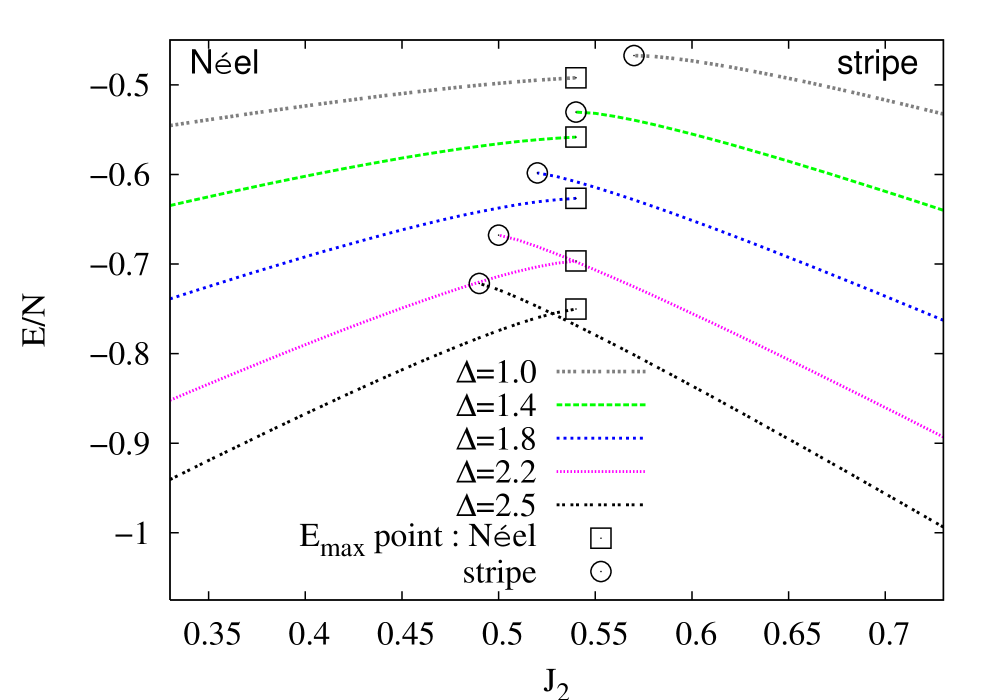
(a) $z$-aligned states

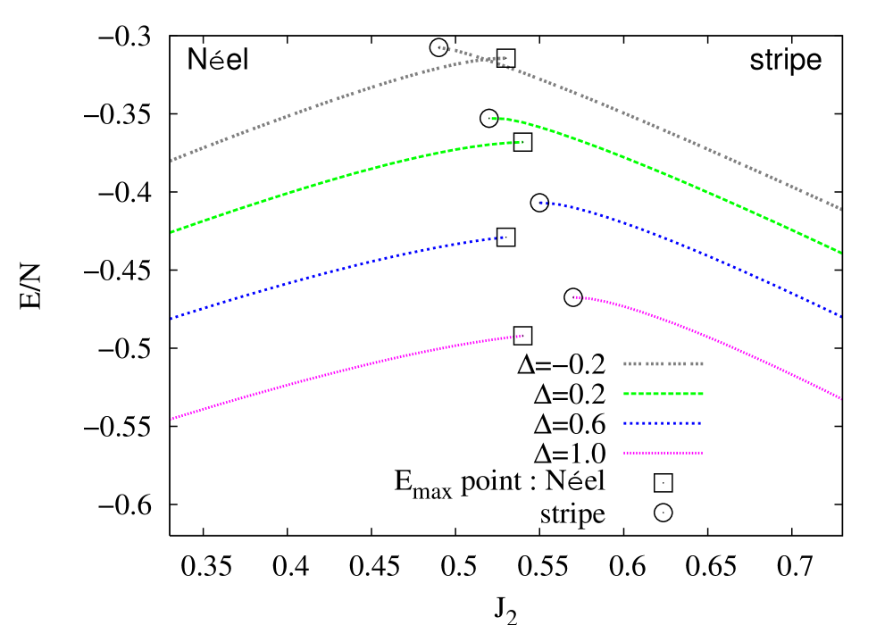
(b) planar $x$-aligned states

Figure 2: Extrapolated CCM LSUB$n$ results using the $z$-aligned and planar $x$-aligned states for the gs energy per spin, $E/N$, for the Néel and stripe phases of the $s=1/2$ $J_{1}^{XXZ}$–$J_{2}^{XXZ}$ model. The LSUB$n$ results are extrapolated in the limit $n\rightarrow\infty$ using the sets $n=\{4,6,8,10\}$ for both the $z$-aligned states and the planar $x$-aligned states. The NN exchange coupling $J_{1}=1$. The meaning of the $E_{\mathrm{max}}$ points shown is described in the text.

shows the extrapolated results for the gs energy per spin as a function of $J_{2}$ (with $J_{1}=1$) for various values of $\Delta$, for the $z$-aligned and planar $x$-aligned model states. For each model state, two sets of curves are shown, one (for smaller values of $J_{2}$) using the Néel state, and the other (for larger values of $J_{2}$) using the stripe state. As we have discussed in detail elsewhere,Bi:1998 ; Ze:1998 ; Fa:2004 the coupled sets of LSUB$n$ equations (6a) have natural termination points (at least for values $n>2$) for some critical value of a control parameter (here the anisotropy, $\Delta$), beyond which no real solutions to the equations exist. The extrapolation of such LSUB$n$ termination points for fixed values of $\Delta$ to the $n\rightarrow\infty$ limit can sometimes be used as a method to calculate the physical phase boundary for the phase with ordering described by the CCM model state being used. However, since other methods exist to define the phase transition points, which are usually more precise and more robust for extrapolation (as we discuss below), we have not attempted such an analysis here.

Instead, in Fig. 2, the $E_{\mathrm{max}}$ points shown, for each set of calculations based on one of the four CCM model states used, are either those natural termination points described above for the highest (LSUB10) level of approximation we have implemented, or the points where the gs energy becomes a maximum should the latter occur first (i.e., as one approaches the termination point). The advantage of this usage of the $E_{\mathrm{max}}$ points is that we do not then display gs energy data in any appreciable regimes where LSUB$n$ calculations with very large values of $n$ (higher than can feasibly be implemented) would not have solutions, by dint of having terminated already.

Curves such as those shown in Fig. 2(a) illustrate very clearly that the corresponding pairs of gs energy curves for the $z$-aligned Néel and stripe phases cross one another for all values of $\Delta$ above some critical value, $\Delta\gtrsim 2.1$. The crossings occur with a clear discontinuity in slope, as is completely characteristic of a first-order phase transition, exactly as observed in the classical (i.e., $s\rightarrow\infty$) case. Furthermore, the direct first-order phase transition between the $z$-aligned Néel and stripe phases that is thereby indicated for all values of $\Delta\gtrsim 2.1$, occurs (for all such values of $\Delta$) very close to the classical phase boundary $J_{2}=\frac{1}{2}$, the point of maximum (classical) frustration. Conversely, curves such as those shown in Fig. 2(a) for values of $\Delta$ in the range $1<\Delta\lesssim 2.1$ also illustrate clearly that the corresponding pairs of gs energy curves for the $z$-aligned Néel and stripe phases do not intersect one another. In this regime we thus have clear preliminary evidence for the opening up of an intermediate phase between the Néel and stripe phases. The corresponding curves in Fig. 2(b) for values of $\Delta<1$ tell a similar story, with an intermediate phase similarly indicated to exist between the $xy$-planar-aligned Néel and stripe phases for values of $\Delta$ in the range $-0.1\lesssim\Delta<1$.

We show in Fig. 3

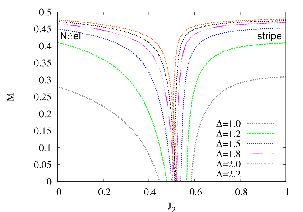
(a) $z$-aligned states

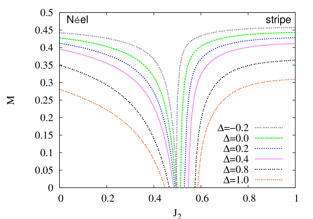
(b) planar $x$-aligned states

Figure 3: Extrapolated CCM LSUB$n$ results using the $z$-aligned and planar $x$-aligned states for the gs staggered magnetization, $M$, for the Néel and stripe phases of the $s=1/2$ $J_{1}^{XXZ}$–$J_{2}^{XXZ}$ model. The LSUB$n$ results are extrapolated in the limit $n\rightarrow\infty$ using the sets $n=\{4,6,8,10\}$ for both the $z$-aligned states and the planar $x$-aligned states. The NN exchange coupling $J_{1}=1$.

corresponding indicative sets of CCM results, based on the same four model states, for the gs order parameter (viz., the staggered magnetization), to those shown in Fig. 2 for the gs energy. The staggered magnetization data completely reinforce the phase structure of the model as deduced above from the gs energy data. Thus, let us now denote by $M_{c}$ the quantum phase transition point deduced from curves such as those shown in Fig. 3, where $M_{c}$ is defined to be either (a) the point where corresponding pairs of CCM staggered magnetization curves (for the same value of $\Delta$), based on the Néel and stripe model states, intersect one another if they do so at a physical value $M\geq 0$; or (b) if they do not so intersect at a value $M\geq 0$, the two points where the corresponding values of the staggered magnetization go to zero.

Clearly, case (a) here corresponds to a direct phase transition between the Néel and stripe phases, which will generally be first-order if the intersection point has a value $M\neq 0$ (and, exceptionally, second-order, if the crossing occurs exactly at $M=0$). On the other hand, case (b) corresponds to the situation where the points where the LRO vanishes for both quasiclassical (i.e., Néel-ordered and stripe-ordered) phases are, at least naively, indicative of a second-order phase transition from each of these phases to some unknown intermediate magnetically-disordered phase. We return to a discussion of the actual order of such transitions in Sec. V. In summary, we hence define the staggered magnetization criterion for a quantum critical point as the point where there is an indication of a phase transition between the two states by their order parameters becoming equal, or where the order parameter vanishes, whichever occurs first. A detailed discussion of this order parameter criterion and its relation to the stricter energy crossing criterion may be found elsewhere.Schm:2006

From curves such as those shown in Fig. 3(a) we see that for $\Delta\lesssim 1.95$ for the $z$-aligned states, there exists an intermediate region between the critical points at which $M\rightarrow 0$ for the Néel and stripe phases. Conversely, for $\Delta\gtrsim 1.95$ the two curves for the order parameters $M$ of the quantum Néel and stripe phases for the same value of $\Delta$ meet at a finite value, $M>0$, as is typical of a first-order transition. Similarly, Fig. 3(b) shows that for the planar $x$-aligned states, there exists an intermediate region between the critical points at which $M\rightarrow 0$ for the Néel and stripe phases for all values of $\Delta$ in the range $-0.15\lesssim\Delta<1$. Again, the two curves for the order parameters $M$ of the Néel and stripe phases for the same value of $\Delta$ intersect at a value $M>0$ for $\Delta\lesssim-0.15$. In order to show more explicitly how the quantum phase transitions are driven by anisotropy, $\Delta$, we display the same data for the extrapolated results for the order parameter, $M$, somewhat differently in Fig. 4,

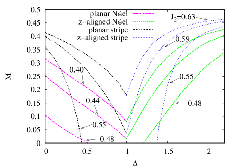
Figure 4: Extrapolated CCM LSUB$n$ results using the $z$-aligned and planar $x$-aligned states for the staggered magnetization versus the anisotropy $\Delta$ for the $s=1/2$ $J_{1}^{XXZ}$–$J_{2}^{XXZ}$ model, for the NN exchange coupling $J_{1}=1$. The LSUB$n$ results are extrapolated in the limit $n\rightarrow\infty$ using the sets $n=\{4,6,8,10\}$ for both the $z$-aligned model states and the planar $x$-aligned model states.

where we plot $M$ as a function of $\Delta$ for various values of $J_{2}$ around the value $J_{2}=0.5$, corresponding to the point of maximum (classical) frustration.

By putting together data of the sort shown in Figs. 2, 3, and 4 we are able to deduce the gs phase diagram of our 2D spin-1/2 $J_{1}^{XXZ}$–$J_{2}^{XXZ}$ model on the square lattice, from our CCM calculations based on the four model states with quasiclassical antiferromagnetic LRO (viz., the Néel and stripe states for both the $z$-aligned and planar $xy$-aligned cases). We show in Fig. 5

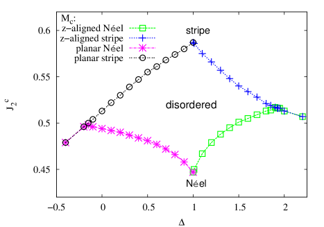
Figure 5: Extrapolated CCM LSUB$n$ results using the $z$-aligned and planar $x$-aligned states for the ground-state phase diagram of the $s=1/2$ $J_{1}^{XXZ}$–$J_{2}^{XXZ}$ model, for the NN exchange coupling $J_{1}=1$. The LSUB$n$ results for the staggered magnetization are extrapolated to the limit $n\rightarrow\infty$ using the sets $n=\{4,6,8,10\}$ for both the $z$-aligned model states and the planar $x$-aligned model states. $M_{c}\equiv$ magnetization critical point, defined in the text.

the zero-temperature gs phase diagram, as deduced from the order parameter criterion, and using our extrapolated LSUB$n$ data sets with $n=\{4,6,8,10\}$, shown as the critical value $J_{2}^{c}$ for the NNN exchange coupling $J_{2}$ as a function of anisotropy $\Delta$ (with NN exchange coupling strength $J_{1}=1$). Very similar results are obtained from using the energy criterion, where it can be applied (viz., along the transition lines between quasiclassical states with magnetic LRO). In order to test the accuracy of our results, particularly the positions of the phase boundaries shown in Fig. 5, we have also performed extrapolations using the LSUB$n$ data sets with $n=\{2,4,6,8,10\}$ and $n=\{6,8,10\}$ for both the energy criterion and the order parameter criterion. In general terms we find that the results are remarkably robust, and the error bars quoted below are based on such an analysis.

For the case of the $z$-aligned states, all of our results provide clear and consistent evidence for an upper quantum triple point (QTP) at ($\Delta^{c}=2.05\pm 0.15,J_{2}^{c}=0.530\pm 0.015$) (for $J_{1}=1$). For $1<\Delta\lesssim 2.0$, there exists an intermediate paramagnetic (magnetically-disordered) quantum phase, separating the Néel and stripe phases. This intermediate phase disappears for $\Delta\gtrsim 2.0$, and both our energy and order parameter criteria give clear and unequivocal evidence for a direct first-order quantum phase transition between the two quasiclassical antiferromagnetic states in this regime, just as in the corresponding classical model (i.e., with $s\rightarrow\infty$). The phase boundary approaches the classical line $J_{2}^{c}=0.5$ as $\Delta\rightarrow\infty$.

Similarly, for the case of the $xy$-planar-aligned phases, a second (lower) QTP occurs at ($\Delta^{c}=-0.10\pm 0.15,J_{2}^{c}=0.505\pm 0.015$) (for $J_{1}=1$), with an intermediate disordered phase existing in the region $-0.1\lesssim\Delta<1$. The $z$-aligned and $xy$-planar-aligned phases meet precisely at $\Delta=1$, just as in the classical case. Exactly at the isotropic point $\Delta=1$, where the model becomes just the original $J_{1}$–$J_{2}$ model, the disordered phase exists for the largest range of values of $J_{2}$, $J_{2}^{c_{1}}<J_{2}<J_{2}^{c_{2}}$, as can be clearly seen from Fig. 5. For the pure $J_{1}$–$J_{2}$ model our calculations yield the values $J_{2}^{c_{1}}/J_{1}=0.44\pm 0.01$ and $J_{2}^{c_{2}}/J_{1}=0.59\pm 0.01$ that demarcate the phase boundaries for the disordered phase, in complete agreement with both our own earlier work and that of others that we have already discussed in Sec. I.

V Discussion and Conclusions

We have shown in detail how, as expected, the quantum fluctuations present in the spin-1/2 $J_{1}$–$J_{2}$ model on the 2D square lattice, that has become an archetypal model for studying the interplay between quantum fluctuations and frustration, can be tuned by the introduction of spin anisotropy. We have clearly confirmed our prior expectation that anisotropy reduces the quantum fluctuations. Thus, for both the cases $\Delta>1$ and $0<\Delta<1$, the intermediate paramagnetic phase present in the pure $J_{1}$–$J_{2}$ model is observed to shrink to a smaller range of values of $J_{2}/J_{1}$ centered near to the point of maximal classical frustration, $J_{2}^{c}/J_{1}=\frac{1}{2}$, that marks the classical phase boundary between the Néel-ordered and collinear stripe-ordered phases.

We have seen that the intermediate disordered phase disappears precisely at two quantum triple points at $\Delta^{c}=-0.10\pm 0.15$ and $\Delta^{c}=2.05\pm 0.15$, and that for values of $\Delta$ outside the range spanned by these values the intermediate phase is totally absent. In particular, for $\Delta\gtrsim 2.0$ we find unequivocal evidence for a first-order phase transition between the Néel and collinear stripe phases. This direct first-order phase transition between states of different quasiclassical antiferromagnetic ordering is very similar to what has been observed in another similar extension of the spin-1/2 $J_{1}$–$J_{2}$ model on a square lattice, namely the so-called $J_{1}$–$J_{2}$–$J_{\perp}$ model on a stacked square lattice where we now introduce a (weak) interlayer coupling through NN bonds of strength $J_{\perp}$. The quantum fluctuations in the $J_{1}$–$J_{2}$ model are tuned here by the parameter $J_{\perp}$. An analysis of this modelSchm:2006 found that the intermediate region of disordered paramagnetic phase, $\alpha^{c_{1}}<J_{2}/J_{1}<\alpha^{c_{2}}$, in the pure $J_{1}$–$J_{2}$ model now shrinks as the interlayer coupling strength $J_{\perp}$ is increased. The second-order phase transition for the Néel-ordered phase to the paramagnetic phase disappears for $J_{\perp}/J_{1}$ above some critical value (estimated to be in the range 0.2–0.3) marking a QTP in the $J_{2}$–$J_{\perp}$ plane (with $J_{1}\equiv 1$). Above the QTP there is again a direct first-order phase transition between the two phases of different quasiclassical antiferromagnetic LRO.

On the other hand this scenario of a first-order phase transition between the two states of different quasiclassical LRO may be contrasted with the situation observed in yet another generalization of the pure spin-1/2 $J_{1}$–$J_{2}$ model on a square lattice, namely the so-called $J_{1}$–$J_{1}^{\prime}$–$J_{2}$ model that we have briefly discussed in Sec. I. In this case the quantum fluctuations are tuned by introducing a spatial anisotropy so that the NN bonds have different strengths in the intrachain ($J_{1}$) and interchain ($J_{1}^{\prime}$) directions on the square lattice. A similar CCM analysis of the spin-1/2 version of this model by some of the present authorsBi:2007_j1j2j3_spinHalf again found a QTP in the $J_{2}$–$J_{1}^{\prime}$ plane (with $J_{1}\equiv 1$), now below which the disordered paramagnetic phase disappears, and there is again a direct phase transition between the quasiclassical Néel and stripe-ordered phases with magnetic LRO. However, the surprising and novel situation found here was the existence of strong evidence for the phase transition in this case to be second-order, and hence inexplicable by standard Ginzburg-Landau theory, as discussed more fully in Sec. I above.

Having discussed the transition line between the two phases of quasiclassical antiferromagnetic LRO in the phase diagram in the $J_{2}$–$\Delta$ plane of our spin-1/2 $J_{1}^{XXZ}$–$J_{2}^{XXZ}$ model on the 2D square lattice, we turn our attention to the four phase boundary lines shown in Fig. 5 that delimit the region of existence for the intermediate disordered paramagnetic phase. As has been explained in Ref. [Schm:2006, ] a judicious combination of the CCM energy data with the CCM order parameter data can shed light on the nature of the phase transitions between the quasiclassically long-range-ordered phases and the paramagnetic phase. The method for so doing relies essentially on the fact that although we perform our CCM calculations with model (or reference) states with quasiclassical LRO, one knowsBi:1998_PRB58 ; Ze:1998 ; Kr:2000 ; Dar:2005 that one can also reliably use such calculations in parameter regimes where all semblance of the quasiclassical LRO is destroyed. Thus, what is required for the CCM equations to converge to a solution is a sufficient overlap between the wave functions of the model (reference) state $|\Phi\rangle$ and the true GS $|\Psi\rangle$. The termination points of the CCM LSUB$n$ equations discussed above are indicators of where this condition breaks down. Thus, provided that the CCM LSUB$n$ equations converge and yield extrapolated solutions far enough beyond the points $M_{c}$ where the order parameter vanishes, we can also determine whether the solution based on the Néel-ordered or the stripe-ordered model state has lower energy.

We find in this way that there are indicators of a very narrow region where the gs energy obtained with the Néel model state might be slightly lower in energy than that obtained with the collinear striped model state, even in regions (close to) where the Néel order parameter has already gone to zero, but where the stripe order parameter is still nonzero. As explained in more detail in Ref. [Schm:2006, ], the use of this evidence here points towards the zero-temperature phase transitions from Néel LRO to quantum paramagnetic disorder being second-order, while the transitions from quantum paramagnetic disorder to collinear stripe order are possibly (rather weakly) first-order rather than second-order. We stress, however, that the analysis here is very sensitive to the accuracy of our results, and the evidence for the nature of these quantum phase transitions involving the quantum paramagentic state in the regime $-0.1\lesssim\Delta\lesssim 2.0$ is less compelling than that for the transition between the two quasiclassically ordered states being first-order in the regime $\Delta\gtrsim 2.0$.

The only other analysis of the current spin-1/2 $J_{1}^{XXZ}$–$J_{2}^{XXZ}$ model on the square lattice of which we are awareBe:1998 has been performed at the very low level of lowest-order spin-wave theory (LSWT). For the case studied here of equal spin-anisotropy parameters in the NN and NNN exchange bonds, these authors have only investigated the case $\Delta>1$, for which they find an (upper) QTP at a very small value of the anisotropy parameter, $\Delta^{c}_{(u)}\approx 1.048$, much smaller than the corresponding value $\Delta^{c}_{(u)}=2.05\pm 0.15$ obtained by us for the upper QTP. Such an extreme fragility or sensitivity of the paramagnetic phase to spin anisotropy is not easy to understand. In the face of our own much more accurate calculations it would seem simply to be an artefact of the LSWT approximation. On the other hand, the LSWT analysis does give the same qualitative trends as found by us for the phase transitions in the range $\Delta>1$, viz., a second-order transition between the Néel-ordered and disordered phases, and a first-order transition between the disordered and collinear stripe-ordered phases for $1<\Delta<\Delta^{c}_{(u)}$, and a direct first-order transition between the Néel-ordered and collinear stripe-ordered phases for $\Delta>\Delta^{c}_{(u)}$.

It is perhaps worth noting at this point in the context of spin-wave theory (SWT) that IgarashiIg:1993 has shown that whereas its lowest-order (or linear) version (LSWT) works quite well when applied to the isotropic Heisenberg model with NN couplings only, it consistently oversestimates the quantum fluctuations in the pure (isotropic) $J_{1}$–$J_{2}$ model as the frustration $J_{2}/J_{1}$ increases. Thus, he showed by going to higher orders in SWT in powers of $1/s$, where LSWT is the leading order, that the expansion converges reasonably well for values of $\alpha\equiv J_{2}/J_{1}\lesssim 0.35$, but for larger values of the frustration parameter $\alpha$, including the point $\alpha=0.5$ of maximum classical frustration, the series loses stability. He showed for the $s=\frac{1}{2}$ $J_{1}$–$J_{2}$ model that whereas LSWT predictsCh:1988 a value of $\alpha^{c_{1}}\approx 0.38$ at which the transition from the Néel-ordered phase to the disordered phase occurs, the higher-order corrections to SWT for $\alpha\lesssim 0.4$ make the Néel-ordered phase more stable than predicted by LSWT. This is precisely in agreement with our own predicted value of $\alpha^{c_{1}}=0.44\pm 0.01$ for the $s=\frac{1}{2}$ $J_{1}$–$J_{2}$ model on the square lattice. He concludes that any predictions from SWT for the $J_{1}$–$J_{2}$ model on the square lattice are likely to be unreliable for values $J_{2}/J_{1}\gtrsim 0.4$.

For reasons unclear to us, the authors of Ref. [Be:1998, ] never investigated the regime with $\Delta<1$, for which we find a lower QTP at $\Delta^{c}_{(l)}=-0.10\pm 0.15$, $J_{2(l)}^{c}=0.505\pm 0.015$. Clearly, our results are consistent with this lower QTP occurring exactly at the isotropic XY point (i.e., $\Delta=0$) of the model, and also exactly at the point of maximal classical frustration, $J_{2}=\frac{1}{2}$. A more detailed theoretical investigation of the corresponding $J_{1}^{XX}$–$J_{2}^{XX}$ model is clearly warranted by our results.

Finally, we note that in our analysis here we have relied on two of the unique strengths of the CCM, namely its ability to deal with highly frustrated systems as readily as unfrustrated ones, and its use from the outset of infinite lattices. In turn, these features lead to its ability to yield accurate phase boundaries even in the very delicate regions near quantum triple points. Our own results for the gs energy and staggered magnetization from four sets of independent calculations based on different reference states provide us with a set of internal checks that lead us to believe that we now have a self-consistent and robust description of this rather challenging model system.

References

- (1) Quantum Magnetism, edited by U. Schollwöck, J. Richter, D.J.J. Farnell, and R.F. Bishop, Lecture Notes in Physics 645 (Springer-Verlag, Berlin, 2004).
- (2) S. Tomonaga, Prog. Theor. Phys. 5, 544 (1950).
- (3) J.M. Luttinger, J. Math. Phys. 4, 1154 (1963).
- (4) P.W. Anderson, Science 235, 1196 (1987).
- (5) E. Manousakis, Rev. Mod. Phys. 63, 1 (1991).
- (6) P. Chandra and B. Doucot, Phys. Rev. B 38, 9335 (1988).
- (7) E. Dagotto and A. Moreo, Phys. Rev. Lett. 63, 2148 (1989).
- (8) P. Chandra, P. Coleman, and A.I. Larkin, Phys. Rev. Lett. 64, 88 (1990).
- (9) H.J. Schulz and T.A.L. Ziman, Europhys. Lett. 18, 355 (1992); H.J. Schulz, T.A.L. Ziman, and D. Poilblanc, J. Phys. I France 6, 675 (1996).
- (10) J. Richter, Phys. Rev. B 47, 5794 (1993); J. Richter, N.B. Ivanov, and K. Retzlaff, Europhys. Lett. 25, 545 (1994).
- (11) J. Igarishi, J. Phys. Soc. Japan 62, 4449 (1993).
- (12) R.F. Bishop, D.J.J. Farnell, and J.B. Parkinson, Phys. Rev. B 58, 6394 (1998).
- (13) L. Capriotti and S. Sorella, Phys. Rev. Lett. 84, 3173 (2000).
- (14) L. Capriotti, F. Becca, A. Parola, and S. Sorella, Phys. Rev. Lett. 87, 097201 (2001).
- (15) L. Siurakshina, D. Ihle, and R. Hayn, Phys. Rev. B 64, 104406 (2001).
- (16) O.P. Sushkov, J. Oitmaa, and Z. Weihong, Phys. Rev. B 63, 104420 (2001).
- (17) F. Becca and F. Mila, Phys. Rev. Lett., 89, 037204 (2002).
- (18) R.R.P. Singh, W. Zheng, J. Oitmaa, O.P. Sushkov, and C.J. Hamer, Phys. Rev. Lett. 91, 017201 (2003).
- (19) G.M. Zhang, H. Hu, and L. Yu, Phys. Rev. Lett. 91, 067201 (2003).
- (20) G. Misguich and C. Lhuillier, in Frustrated Spin Systems, edited by H.T. Diep (World Scientific, Singapore, 2005), p.229.
- (21) P. Carretta, N. Papinutto, C.B. Azzoni, M.C. Mozzati, E. Pavarini, S. Gonthier, and P. Millet, Phys. Rev. B 66, 094420 (2002).
- (22) R. Melzi, P. Carretta, A. Lascialfari, M. Mambrini, M. Troyer, P. Millet, and F. Mila, Phys. Rev. Lett. 85, 1318 (2000).
- (23) H. Rosner, R.R.P. Singh, W.H. Zheng, J. Oitmaa, S.-L. Drechsler, and W.E. Pickett, Phys. Rev. Lett. 88, 186405 (2002).
- (24) A.W. Sandvik, Phys. Rev. B 56, 11678 (1997).
- (25) J. Richter, J. Schulenburg, and A. Honecker, in Quantum Magnetism, edited by U. Schollwöck, J. Richter, D.J.J. Farnell, and R.F. Bishop, Lecture Notes in Physics 645 (Springer-Verlag, Berlin, 2004), p.85.
- (26) Z. Weihong, J. Oitmaa, and C.J. Hamer, Phys. Rev. B 43, 8321 (1991).
- (27) R.F. Bishop, D.J.J. Farnell, S.E. Krüger, J.B. Parkinson, J. Richter, and C. Zeng, J. Phys.: Condens. Matter 12, 6887 (2000).
- (28) J. Richter, R. Darradi, R. Zinke, and R.F. Bishop, Int. J. Mod. Phys. B 21, 2273 (2007).
- (29) R.F. Bishop and D.J.J. Farnell, Int. J. Mod. Phys. B – in press (2008).
- (30) C.J. Hamer, Z. Weihong, and P. Arndt, Phys. Rev. B 46, 6276 (1992).
- (31) J. Villain, J. Phys. (Paris) 38, 26 (1977); J. Villain, R. Bidaux, J.P. Carton, and R. Conte, J. Phys. (Paris) 41, 1263 (1980).
- (32) E. Shender, Sov. Phys. JETP 56, 178 (1982).
- (33) N. Read and S. Sachdev, Phys. Rev. Lett. 66, 1773 (1991).
- (34) R.R.P. Singh, Z. Weihong, C.J. Hamer, and J. Oitmaa, Phys. Rev. B 60, 7278 (1999).
- (35) V.N. Kotov, J. Oitmaa, O. Sushkov, and Z. Weihong, Phil. Mag. B 80, 1483 (2000).
- (36) J. Sirker, Z. Weihong, O.P. Sushkov, and J. Oitmaa, Phys. Rev. B 73, 184420 (2006).
- (37) M.E. Zhitomirski and K. Ueda, Phys. Rev. B 54, 9007 (1996).
- (38) T. Senthil, A. Vishwanath, L. Balents, S. Sachdev, and M.P.A. Fisher, Science 303, 1490 (2004); T. Senthil, L. Balents, S. Sachdev, A. Vishwanath, and M.P.A. Fisher, Phys. Rev. B 70, 144407 (2004).
- (39) O.P. Sushkov, J. Oitmaa, and Z. Weihong, Phys. Rev. B 66, 054401 (2002).
- (40) A.A. Nersesyan and A.M. Tsvelik, Phys. Rev. B 67, 024422 (2003).
- (41) P. Sindzingre, Phys. Rev. B 69, 094418 (2004).
- (42) O.A. Starykh and L. Balents, Phys. Rev. Lett. 93, 127202 (2004).
- (43) S. Moukouri, J. Stat. Mech. P02002 (2006).
- (44) R.F. Bishop, P.H.Y. Li, R. Darradi, and J. Richter, J. Phys.: Condens. Matter 20 – in press (2008) (and see arXiv:0705.2201v4 [cond-mat.str-el]).
- (45) R.F. Bishop, P.H.Y. Li, R. Darradi, and J. Richter, arXiv:0802.2566v2 [cond-mat.str-el] (2008)
- (46) T. Roscilde, A. Feiguin, A.L. Chernyshev, S. Liu, and S. Haas, Phys. Rev. Lett. 93, 017203 (2004).
- (47) J.R. Viana and J.R. de Sousa, Phys. Rev. B 75, 052403 (2007).
- (48) A. Benyoussef, A. Boubekri, and H. Ez-Zahraouy, Phys. Lett. A 238, 398 (1998).
- (49) R. Darradi, J. Richter, and S.E. Krüger, J. Phys.: Condens. Matter 16, 2681 (2004).
- (50) R. Schmidt, J. Schulenburg, J. Richter, and D.D. Betts, Phys. Rev. B 66, 224406 (2002).
- (51) J. Oitmaa and W. Zheng, Phys. Rev. B 69, 064416 (2004).
- (52) R.F. Bishop, Theor. Chim. Acta 80, 95 (1991).
- (53) R.F. Bishop, in Microscopic Quantum Many-Body Theories and Their Applications, edited by J. Navarro and A. Polls, Lecture Notes in Physics 510 (Springer-Verlag, Berlin, 1998), p.1.
- (54) C. Zeng, D.J.J. Farnell, and R.F. Bishop, J. Stat. Phys. 90, 327 (1998).
- (55) S.E. Krüger, J. Richter, J. Schulenburg, D.J.J. Farnell, and R.F. Bishop, Phys. Rev. B 61, 14607 (2000).
- (56) D.J.J. Farnell, R.F. Bishop, and K.A. Gernoth, J. Stat. Phys. 108, 401 (2002).
- (57) D.J.J. Farnell and R.F. Bishop, in Quantum Magnetism, edited by U. Schollwöck, J. Richter, D.J.J. Farnell, and R.F. Bishop, Lecture Notes in Physics 645 (Springer-Verlag, Berlin, 2004), p.307.
- (58) R. Darradi, J. Richter, and D.J.J. Farnell, Phys. Rev. B 72, 104425 (2005).
- (59) D. Schmalfuß, R. Darradi, J. Richter, J. Schulenburg, and D. Ihle, Phys. Rev. Lett. 97, 157201 (2006).
- (60) We use the program package “Crystallographic Coupled Cluster Method” (CCCM) of D.J.J. Farnell and J. Schulenburg, see http://www-e.uni-magdeburg.de/jschulen/ccm/index.html.
- (61) R. Zinke, J. Schulenburg, and J. Richter, Eur. Phys. J. B 61, 147 (2008).