Kinetics of spin coherence of electrons in $n$-type InAs quantum wells under intense terahertz laser fields

Abstract

Spin kinetics in $n$-type InAs quantum wells under intense terahertz laser fields is investigated by developing fully microscopic kinetic spin Bloch equations via the Floquet-Markov theory and the nonequilibrium Green’s function approach, with all the relevant scattering, such as the electron-impurity, electron-phonon, and electron-electron Coulomb scattering explicitly included. We find that a finite steady-state terahertz spin polarization induced by the terahertz laser field, first predicted by Cheng and Wu [Appl. Phys. Lett. 86, 032107 (2005)] in the absence of dissipation, exists even in the presence of all the scattering. We further discuss the effects of the terahertz laser fields on the spin relaxation and the steady-state spin polarization. It is found that the terahertz laser fields can strongly affect the spin relaxation via hot-electron effect and the terahertz-field-induced effective magnetic field in the presence of spin-orbit coupling. The two effects compete with each other, giving rise to non-monotonic dependence of the spin relaxation time as well as the amplitude of the steady state spin polarization on the terahertz field strength and frequency. The terahertz field dependences of these quantities are investigated for various impurity densities, lattice temperatures, and strengths of the spin-orbit coupling. Finally, the importance of the electron-electron Coulomb scattering on spin kinetics is also addressed.

I Introduction

Generating and manipulating spin coherence of electrons is one of the most important research focuses of semiconductor spintronics community.spintronics ; wolf ; dot There have been many proposals to use electric field rather than magnetic field to generate and manipulate electron spin coherence.Salis ; Tokura ; Rashba0 ; Rashba1 ; Rashba2 ; Cheng ; Rashba3 ; Duckheim ; yzhou ; Rodriguez ; Jiang ; Golovach ; Fabian ; Bulaev ; wu-trans-pulse ; Pershin The mechanism of such proposals is that when the spin degree of freedom is coupled to the orbital degree of freedom via spatial varying $g$-tensor (or magnetic field) or spin-orbit coupling (SOC) (such as the Rashba,Rashba the DresselhausDresselhaus and the strain-inducedopt-or SOC), the electric field can act directly on spin through driving the orbital motion. Recently, Kato et al. achieved coherent spin rotation via gigahertz electric field applied along the growth direction of the $g$-tensor engineered GaAs/Al_xGa_1-xAs parabolic quantum wells.Kato0 It has also been demonstrated experimentally that the SOC can enable electrical control of spin coherence without magnetic field.Kato1 ; Crooker ; Meier Rashba and Efros showed that even preferable to ac magnetic fields, ac electric fields can efficiently induce spin resonance in the presence of SOC in quantum wells, especially when the ac electric field is the in-plane one.Rashba0 ; Rashba1 ; Rashba2 ; Rashba3 This effect is called electric dipole spin resonance which was later observed by Kato et al. in bulk GaAs,Kato1 Meier et al. in GaAs/InGaAs quantum wells,Meier and Nowack et al. in GaAs quantum dots.Nowack In these investigations, only weak electric fields are applied.

Recently, Cheng and Wu showed theoretically that in InAs quantum wells, a strong in-plane terahertz (THz) electric field ($\sim 1$ kV/cm) can induce a large spin polarization ($\sim 10$ %) oscillating at the same frequency of the THz driving field when dissipations are not considered.Cheng This indicates that using strong THz electric field is a promising way to achieve high-frequency spin manipulation and spin generation in InAs-based nanostructures where the spin splitting is of the order of THz.Grundler ; Sato They also showed that the strong THz field can greatly modify the density of states via the dynamical Franz-Keldysh effect,Jauho the sideband effectsideband and the ac Stark effect.ACStark ; ACReview1 ; ACReview2 ; Ganichevbook Later, Jiang et al. predicted similar effects in singly charged InAs quantum dots.Jiang As the density of states of the electron spin system is greatly modified by the intense THz fields, the dissipation effects may also be manipulated. However, up till now there is few study on the dissipative kinetics of strongly-driven electron spin system, especially from a fully microscopic approach. Previously, we have demonstrated that intense THz driving field in InAs quantum dots can elongate spin relaxation time (SRT) by more than one order of magnitude.Jiang2 The underlying physics is that the sideband effect strongly modulates the phonon-induced spin-flip transition rates. The effects of intense THz fields on spin relaxation in two dimensional electron system (2DES) are still unknown. The spin relaxation mechanism in 2DES is quite different from that in quantum dots. In the driving-field-free limit, it is widely accepted that spin relaxation in 2DES is dominated by D’yakonov-Perel’ (DP) mechanism.spintronics ; opt-or Previously, spin relaxation and spin dephasing have been closely studied using the kinetic spin Bloch equation approach developed by Wu et al.wu-review in intrinsic, $n$-type and $p$-type semiconductors, in both Markovian and non-Markovian limits, even in systems far away from the equilibrium (under strong static electric field or with high spin polarization).wu-early ; wu-later ; wu-hole ; wu-highP ; wu-hot-e ; wu-helix ; wu-lowT ; wu-nonM ; wu-bap The theory, which includes all relevant scattering (such as the electron-impurity, electron-phonon and electron-electron Coulomb scattering) explicitly, agrees very well with experiments.wu-lowT ; wu-Exp-Aniso Many predictions from the theory have recently been confirmed experimentally.david ; wu-Exp-HighP

In this work, we first extend the theory to study the spin kinetics under intense THz laser fields in InAs quantum wells. The kinetic spin Bloch equations are derived in the spirit of the Floquet-Markov approachFM via nonequilibrium Green function method.Haugbook The Floquet-Markov approach combines the Floquet theory, which solves the time-dependent Schrödinger equation of the strongly-driven system non-perturbatively,Shirley ; ACReview1 with the Born-Markov approximation which is widely used in the derivation of the equation of motion for the reduced density matrix of the concerned system.QN The theory is frequently applied in the study of dissipative dynamics of strongly-driven systems.ACReview1 ; ACReview2 ; Jiang2 With the extended kinetic spin Bloch equations, we are able to investigate the effect of the strong THz fields on spin kinetics. We show that the steady-state THz spin polarization induced by the THz laser field, first predicted by Cheng and Wu in the dissipation-free case,Cheng still exists in the presence of the full dissipation. Moreover, we investigate how this spin polarization as well as the spin relaxation are manipulated by the external THz laser fields under various conditions. The predicted spin dynamics can be readily confirmed by Faraday and/or Kerr rotation measurementsFR ; KR under intense THz irradiation.

The paper is organized as follows: In Sec. II, we set up the model and establish the kinetic spin Bloch equations. In Sec. III, we present our numerical results. We conclude and discuss in Sec. IV.

II Model and Formalism

II.1 Model

We consider a 2DES confined in InAs quantum well. The confinement along the $z$ direction is so strong (well width $a=5$ nm) that only the lowest subband is considered. The THz electric field ${\bf E}_{THz}(t)={\bf E}\sin(\Omega t)$ is applied in the quantum well plane. Here $\Omega=2\pi\nu$ is the angular velocity, with $\nu$ being the frequency of the THz field. In experiments, the THz field can be provided by the free electron laser.Ramian In the Coulomb gauge, the vector potential is ${\bf A}(t)={\bf E}\cos(\Omega t)/\Omega$ and the scalar potential is $\Phi=0$. In InAs quantum wells, the dominant SOC is the Rashba SOC.Rashba As the Rashba SOC is rotational invariant, we take ${\bf E}_{THz}$ along $x$ axis. The total Hamiltonian is then

$$H=H_{e}+H_{ei}+H_{ee}+H_{ep}+H_{ph}.$$ (1)

Here $H_{ph}=\sum_{\lambda,{\bf Q}}\omega_{\lambda,{\bf Q}}\hat{a}_{\lambda,{\bf Q}}^{\dagger}\hat{a}_{\lambda,{\bf Q}}$ represents the phonon Hamiltonian (We take $\hbar\equiv 1$ throughout the paper). $H_{ei}=\sum_{{\bf k}{\bf Q},\sigma,j}U_{{\bf Q}}I(iq_{z})e^{-i{\bf Q}\cdot{\bf R}_{j}}\hat{\sl c}^{\dagger}_{{\bf k}\sigma}\hat{\sl c}_{{\bf k}-{\bf q}\sigma}$, $H_{ee}=\frac{1}{2}\sum_{{\bf k}{\bf k}^{\prime}{\bf Q},\sigma\sigma^{\prime}}V_{{\bf Q}}|I(iq_{z})|^{2}\hat{\sl c}^{\dagger}_{{\bf k}\sigma}\hat{\sl c}^{\dagger}_{{\bf k}^{\prime}\sigma^{\prime}}\hat{\sl c}_{{\bf k}^{\prime}-{\bf q}\sigma^{\prime}}\hat{\sl c}_{{\bf k}+{\bf q}\sigma}$ and $H_{ep}=\sum_{\lambda,{\bf Q}{\bf k}}M_{\lambda,{\bf Q}}I(iq_{z})(\hat{a}_{\lambda,{\bf Q}}+\hat{a}_{\lambda,{\bf-Q}}^{\dagger})\hat{\sl c}^{\dagger}_{{\bf k}\sigma}\hat{\sl c}_{{\bf k}-{\bf q}\sigma}$ denote the electron-impurity, electron-electron and electron-phonon interactions, respectively. Here, $\omega_{\lambda,{\bf Q}}$ is the phonon frequency, $\hat{a}_{\lambda,{\bf Q}}$ ($\hat{\sl c}_{{\bf k}\sigma}$) is the phonon (electron) annihilation operator with $\lambda$ being the phonon branch index ($\sigma$ denoting the electron spin index), ${\bf R}_{j}$ stands for the position of $j$th impurity, ${\bf Q}=({\bf q},q_{z})$ is the three-dimensional momentum whereas ${\bf q}$ and ${\bf k}$’s are the two-dimensional ones along the well plane. $I(iq_{z})=(\frac{2\pi}{a})^{2}(e^{iq_{z}a}-1)/\{iq_{z}a[(\frac{2\pi}{a})^{2}-q_{z}^{2}]\}$ is the form factor of the lowest subband. The matrix elements $V_{{\bf Q}}$, $U_{{\bf Q}}$ for electron-electron and electron-impurity interactions as well as $M_{\lambda,{\bf Q}}$ for the electron–longitudinal-optical-phonon (electron–LO-phonon) interaction can be found in Ref. wu-hot-e, and the ones for the electron–acoustic-phonon interaction can be found in Ref. wu-lowT, . We apply the random phase approximation in the screening of the Coulomb potential.wu-lowT

The electron Hamiltonian can be written as

$$H_{e}=\sum_{{\bf k}\sigma\sigma^{\prime}}H_{0}^{\sigma\sigma^{\prime}}({\bf k},t)\hat{\sl c}^{\dagger}_{{\bf k}\sigma}\hat{\sl c}_{{\bf k}\sigma^{\prime}},$$ (2)

where

$$\hat{H}_{0}({\bf k},t)=\frac{({\bf k}+e{\bf A}(t))^{2}}{2m^{\ast}}\mbox{\boldmath$\hat{1}$\unboldmath}+\alpha_{R}\Big{[}\hat{\sigma}_{x}k_{y}$$

$$\hskip 42.67912pt\mbox{}-\hat{\sigma}_{y}(k_{x}+eA(t))\Big{]}$$

$$=\Big{[}\varepsilon_{\bf k}+\gamma_{E}k_{x}\Omega\cos(\Omega t)+E_{em}(1+\cos(2\Omega t))\Big{]}\mbox{\boldmath$\hat{1}$\unboldmath}$$

$$\mbox{}+\alpha_{R}(\hat{\sigma}_{x}k_{y}-\hat{\sigma}_{y}k_{x})-\alpha_{R}\hat{\sigma}_{y}eE\cos(\Omega t)/\Omega.$$ (3)

Here $\varepsilon_{\bf k}=\frac{{\bf k}^{2}}{2m^{\ast}}$, $\gamma_{E}=\frac{eE}{m^{\ast}\Omega^{2}}$ and $E_{em}=\frac{e^{2}E^{2}}{4m^{\ast}\Omega^{2}}$. It is noted that the last term manifests that the THz electric field acts as a THz magnetic field along the $y$ axis

$$B_{\mbox{eff}}=2\alpha_{R}eE\cos(\Omega t)/\left(|g|\mu_{B}\Omega\right),$$ (4)

where $g$ is the electron $g$-factor. We will show later that this THz-field-induced effective magnetic field has many important effects on spin kinetics. The term proportional to $E_{em}$ is responsible for the dynamical Franz-Keldysh effect.Jauho ; Cheng This term does not contain any dynamic variable of the electron system and thus has no effect on the kinetics of the electron system. Usually, the largest time-periodic term is the term $\gamma_{E}k_{x}\Omega\cos(\Omega t)$, where the sideband effect mainly comes from. Under an intense THz field, this term can be comparable to or larger than $\varepsilon_{\bf k}$. It should be noted that this anisotropic term breaks down $k_{x}\to-k_{x}$ symmetry of the Hamiltonian. We will show later that this asymmetry leads to nonzero value of the average of $k_{x}$ over the electron system when the momentum scattering is included.

The Schrödinger equation for electron with momentum ${\bf k}$ is

$$i\partial_{t}\Psi_{{\bf k}}(t)=\hat{H}_{0}({\bf k},t)\Psi_{{\bf k}}(t).$$ (5)

According to the Floquet theory,Shirley the solution to the above equation reads

$$\Psi_{{\bf k}\eta}(t) = e^{i{\bf k}\cdot{\bf r}-i\varepsilon_{\bf k}t}\phi_{1}(z)\xi_{{\bf k}\eta}(t)$$ (6)

$$\mbox{}\times e^{-i[\gamma_{E}k_{x}\sin(\Omega t)+E_{em}t+E_{em}\frac{\sin(2\Omega t)}{2\Omega}]},$$

with $\eta=\pm$ denoting the spin branch and $\phi_{1}(z)$ being the wavefunction of the lowest subband. $\xi_{{\bf k}\eta}(t)=e^{-iy_{{\bf k}\eta}t}\sum_{n\sigma}\upsilon_{n\sigma}^{{\bf k}\eta}e^{in\Omega t}\chi_{\sigma}$ where $y_{{\bf k}\eta}$ and $\upsilon_{n\sigma}^{{\bf k}\eta}$ are the eigen-value and eigen-vector of the equation

$$(y_{{\bf k}\eta}-n\Omega)\upsilon_{n\sigma}^{{\bf k}\eta} = \frac{i\sigma}{2\Omega}\alpha_{R}eE(\upsilon_{n-1,-\sigma}^{{\bf k}\eta}+\upsilon_{n+1,-\sigma}^{{\bf k}\eta})$$ (7)

$$\mbox{}+\alpha_{R}(k_{y}+i\sigma k_{x})\upsilon_{n,-\sigma}^{{\bf k}\eta}.$$

This equation is equivalent to Eq. (2) in Ref. Cheng, . For each ${\bf k}$, the spinors {$|\xi_{{\bf k}\eta}(t)\rangle$} at any time $t$ form a complete-orthogonal basis of the spin space.ACReview1 ; ACReview2 ; Jiang2 The time evolution operator for state ${\bf k}$ can be written as

$$\hat{U}_{0}^{e}({\bf k},t,0) = \sum_{\eta}|\xi_{{\bf k}\eta}(t)\rangle\langle\xi_{{\bf k}\eta}(0)|e^{-i[\varepsilon_{\bf k}t+\gamma_{E}k_{x}\sin(\Omega t)]}$$ (8)

$$\mbox{}\times e^{-i[E_{em}t+E_{em}\sin(2\Omega t)/(2\Omega)]}.$$

II.2 Kinetic spin Bloch equations

The kinetic spin Bloch equations offer a fully microscopic way to study spin dynamics in semiconductors, even in system with large static electric field where the hot-electron effect is important.wu-hot-e ; wu-lowT The electric field dependence of spin dephasing time in such system was studied first by Weng et al.wu-hot-e for high temperature case and then by Zhou et al.wu-lowT for low temperature case. In these works, the electric field appears only in the driving term. However, in the case of a strong time-periodic field, studies have shown that including this field only in the driving term is insufficient.FM The correct way is to evaluate the collision integral with wavefunctions which are the solutions of the time-dependent Schrödinger equation, i.e., the Floquet wavefunctions, instead of the eigen wavefunctions in the field-free limit.FM ; Haugbook Moreover, the Markovian approximation should be made with respect to the spectrum determined by the Floquet wavefunctions.FM These improvements constitute the Floquet-Markov theory.FM ; ACReview1 Generally, this theory works well when the driven system is in dynamically stable regime and the system-reservoir coupling can be treated perturbatively. Besides giving good results, this approach has the advantage of being easy to handle, compared with the rather complicated path-integral approach,FM which makes it a useful approach in the study of spin kinetics under strong time-periodic fields. In this work, we incorporate the Floquet-Markov approach in setting up the kinetic spin Bloch equations. By making the Markov approximation with respect to the spectrum determined by the Floquet states, we first establish the kinetic equations for the single particle density operator. We then use the Floquet states as basis functions to expand the kinetic equations and obtain the kinetic spin Bloch equations in the presence of the strong THz field. A similar approach has been applied to study the spin relaxation in singly charged quantum dots under intense THz driving fields in our recent work.Jiang2

The kinetic spin Bloch equations for the single particle density operator can be written aswu-review

$$\partial_{t}\hat{\rho}_{{\bf k}}(t)=\partial_{t}\hat{\rho}_{{\bf k}}(t)|_{coh}+\partial_{t}\hat{\rho}_{{\bf k}}(t)|_{scat},$$ (9)

where $\partial_{t}\hat{\rho}_{{\bf k}}(t)|_{coh}$ and $\partial_{t}\hat{\rho}_{{\bf k}}(t)|_{scat}$ are the coherent and scattering terms respectively. $\hat{\rho}_{\bf k}(t)=\sum_{\eta_{1}\eta_{2}}\mbox{Tr}\Big{\{}\hat{c}^{\dagger}_{{\bf k}\eta_{2}}\hat{c}_{{\bf k}\eta_{1}}\hat{\rho}^{e}(t)\Big{\}}|\eta_{1}\rangle\langle\eta_{2}|$ represent the $2\times 2$ single-particle density operators, with $\hat{\rho}^{e}(t)$ and $\{|\eta\rangle\}$ denoting the density operator of the electron system and a complete-orthogonal basis in spin space separately. The explicit form of the equations without the intense driving field can be found in the work of Cheng and Wu.wu-helix The coherent terms, which describe the coherent precession determined by the electron Hamiltonian $H_{e}$ and the Hartree-Fock contribution of the electron–electron Coulomb interaction, can be written as

$$\partial_{t}\hat{\rho}_{{\bf k}}(t)|_{coh}=-i[\hat{H}_{0}({\bf k},t),\hat{\rho}_{{\bf k}}(t)]-i[\hat{\Sigma}^{HF}({\bf k},t),\hat{\rho}_{{\bf k}}(t)].$$ (10)

Here $\hat{\Sigma}^{HF}({\bf k},t)=-\sum_{{\bf k}^{\prime},q_{z}}V_{{{\bf k}-{\bf k}^{\prime}},q_{z}}|I(iq_{z})|^{2}\hat{\rho}_{{\bf k}^{\prime}}(t)$ is the Coulomb Hartree-Fock self-energy. The scattering terms are composed of terms due to the electron-impurity ($\partial_{t}\rho_{{\bf k}}|_{ei}$), electron-phonon ($\partial_{t}\rho_{{\bf k}}|_{ep}$), and electron-electron ($\partial_{t}\rho_{{\bf k}}|_{ee}$) scattering respectively. In the interaction picture, or the “Floquet picture”,

$$\hat{\rho}^{F}_{\bf k}(t)=\hat{U}_{0}^{e\ \dagger}({\bf k},t,0)\hat{\rho}_{\bf k}(t)\hat{U}_{0}^{e}({\bf k},t,0),$$ (11)

and under the generalized Kadanoff-Baym Ansatz,Haugbook these scattering terms read

$$\left.\partial_{t}\rho^{F(\eta\eta^{\prime})}_{{\bf k}}(t)\right|_{ei} = -\sum_{{\bf k}^{\prime},q_{z},n,\eta_{1}\eta_{2}\eta_{3}}\pi n_{i}U^{2}_{{\bf k}-{\bf k}^{\prime},q_{z}}|I(iq_{z})|^{2}\bigg{[}\Big{\{}S^{(\eta\eta_{1})}_{{\bf k},{\bf k}^{\prime}}(t,0)S^{(n)(\eta_{2}\eta_{3})}_{{\bf k}^{\prime},{\bf k}}\delta(n\Omega+\bar{\varepsilon}_{{\bf k}^{\prime}\eta_{2}}-\bar{\varepsilon}_{{\bf k}\eta_{3}})$$ (12)

$$\hskip 28.45274pt\mbox{}\times\Big{(}\rho^{>F(\eta_{1}\eta_{2})}_{{\bf k}^{\prime}}(t)\rho^{<F(\eta_{3}\eta^{\prime})}_{{\bf k}}(t)-\rho^{<F(\eta_{1}\eta_{2})}_{{\bf k}^{\prime}}(t)\rho^{>F(\eta_{3}\eta^{\prime})}_{{\bf k}}(t)\Big{)}\Big{\}}+\Big{\{}\eta\leftrightarrow\eta^{\prime}\Big{\}}^{\ast}\bigg{]},$$

$$\left.\partial_{t}\rho^{F(\eta\eta^{\prime})}_{{\bf k}}(t)\right|_{ep} = -{\sum_{{\bf k}^{\prime},q_{z},n,\lambda,\pm,\eta_{1}\eta_{2}\eta_{3}}\pi|M_{\lambda,{\bf k}-{\bf k}^{\prime},q_{z}}|^{2}|I(iq_{z})|^{2}}\bigg{[}\Big{\{}S^{(\eta\eta_{1})}_{{\bf k},{\bf k}^{\prime}}(t,0)S^{(n)(\eta_{2}\eta_{3})}_{{\bf k}^{\prime},{\bf k}}e^{\mp it\omega_{\lambda,{\bf k}-{\bf k}^{\prime},q_{z}}}$$ (13)

$$\hskip 28.45274pt\mbox{}\times\delta(\pm\omega_{\lambda,{\bf k}-{\bf k}^{\prime},q_{z}}+n\Omega+\bar{\varepsilon}_{{\bf k}^{\prime}\eta_{2}}-\bar{\varepsilon}_{{\bf k}\eta_{3}})\Big{(}N^{\pm}_{\lambda,{\bf k}-{\bf k}^{\prime},q_{z}}\rho^{>F(\eta_{1}\eta_{2})}_{{\bf k}^{\prime}}(t)\rho^{<F(\eta_{3}\eta^{\prime})}_{\bf k}(t)$$

$$\hskip 42.67912pt\mbox{}-N^{\mp}_{\lambda,{\bf k}-{\bf k}^{\prime},q_{z}}\rho^{<F(\eta_{1}\eta_{2})}_{{\bf k}^{\prime}}(t)\rho^{>F(\eta_{3}\eta^{\prime})}_{\bf k}(t)\Big{)}\Big{\}}+{\Big{\{}\eta\leftrightarrow\eta^{\prime}\Big{\}}^{\ast}}\bigg{]},$$

$$\left.\partial_{t}\rho^{F(\eta\eta^{\prime})}_{{\bf k}}(t)\right|_{ee} = -\sum_{{\bf k}^{\prime},{\bf k}^{\prime\prime},n,n^{\prime}}\ \sum_{\eta_{1}...\eta_{7}}\pi\Big{[}\sum_{q_{z}}V_{{\bf k}-{\bf k}^{\prime},q_{z}}|I(iq_{z})|^{2}\Big{]}^{2}\bigg{[}\Big{\{}T^{(\eta\eta_{1})}_{{\bf k},{\bf k}^{\prime}}(t,0)T^{(n^{\prime})(\eta_{2}\eta_{3})}_{{\bf k}^{\prime},{\bf k}}T^{(n-n^{\prime})(\eta_{4}\eta_{5})}_{{\bf k}^{\prime\prime},{\bf k}^{\prime\prime}-{\bf k}+{\bf k}^{\prime}}T^{(\eta_{6}\eta_{7})}_{{\bf k}^{\prime\prime}-{\bf k}+{\bf k}^{\prime},{\bf k}^{\prime\prime}}(t,0)$$ (14)

$$\mbox{}\times\delta(n\Omega+\bar{\varepsilon}_{{\bf k}^{\prime}\eta_{2}}-\bar{\varepsilon}_{{\bf k}\eta_{3}}+\bar{\varepsilon}_{{\bf k}^{\prime\prime}\eta_{4}}-\bar{\varepsilon}_{{\bf k}^{\prime\prime}-{\bf k}+{\bf k}^{\prime}\eta_{5}})\Big{(}\rho^{>F(\eta_{1}\eta_{2})}_{{\bf k}^{\prime}}(t)\rho^{<F(\eta_{3}\eta^{\prime})}_{\bf k}(t)\rho^{<F(\eta_{5}\eta_{6})}_{{\bf k}^{\prime\prime}-{\bf k}+{\bf k}^{\prime}}(t)\rho^{>F(\eta_{7}\eta_{4})}_{{\bf k}^{\prime\prime}}(t)$$

$$\mbox{}-\rho^{<F(\eta_{1}\eta_{2})}_{{\bf k}^{\prime}}(t)\rho^{>F(\eta_{3}\eta^{\prime})}_{\bf k}(t)\rho^{>F(\eta_{5}\eta_{6})}_{{\bf k}^{\prime\prime}-{\bf k}+{\bf k}^{\prime}}(t)\rho^{<F(\eta_{7}\eta_{4})}_{{\bf k}^{\prime\prime}}(t)\Big{)}\Big{\}}+{\Big{\{}\eta\leftrightarrow\eta^{\prime}\Big{\}}^{\ast}}\bigg{]}.$$

In these equations, $N^{\pm}_{\lambda,{\bf k}-{\bf k}^{\prime},q_{z}}=N_{\lambda,{\bf k}-{\bf k}^{\prime},q_{z}}+\frac{1}{2}(1\pm 1)$ stands for the phonon number, $n_{i}$ is the impurity density, $\hat{\rho}^{>}_{\bf k}=\hat{{\bf 1}}-\hat{\rho}_{\bf k}$, $\hat{\rho}^{<}_{\bf k}=\hat{\rho}_{\bf k}$, and $\bar{\varepsilon}_{{\bf k}\eta}=\varepsilon_{{\bf k}}+y_{{\bf k}\eta}$.

$$S^{(\eta_{1}\eta_{2})}_{{\bf k}^{\prime},{\bf k}}(t,0) = \langle\xi_{{\bf k}^{\prime}\eta_{1}}(t)|\xi_{{\bf k}\eta_{2}}(t)\rangle$$ (15)

$$\mbox{}\times e^{i[(\varepsilon_{{\bf k}^{\prime}}-\varepsilon_{\bf k})t+\gamma_{E}\sin(\Omega t)(k_{x}^{\prime}-k_{x})]}$$

$$= \sum_{n}S^{(n)(\eta_{1}\eta_{2})}_{{\bf k}^{\prime},{\bf k}}e^{it(n\Omega+\bar{\varepsilon}_{{\bf k}^{\prime}\eta_{1}}-\bar{\varepsilon}_{{\bf k}\eta_{2}})},$$

with

$$S^{(n)(\eta_{1}\eta_{2})}_{{\bf k}^{\prime},{\bf k}}=\sum_{m\sigma}F^{{\bf k}^{\prime}\eta_{1}\ast}_{m\ \sigma}\ F^{{\bf k}\eta_{2}}_{n+m\ \sigma}.$$ (16)

Here $F^{{\bf k}\eta}_{n\ \sigma}=\sum_{m}\upsilon^{{\bf k}\eta}_{n+m\ \sigma}J_{m}(\gamma_{E}k_{x})$ with $J_{m}(x)$ standing for the $m$th order Bessel function.

$$T^{(\eta_{1}\eta_{2})}_{{\bf k}^{\prime},{\bf k}}(t,0) = \langle\xi_{{\bf k}^{\prime}\eta_{1}}(t)|\xi_{{\bf k}\eta_{2}}(t)\rangle e^{i(\varepsilon_{{\bf k}^{\prime}}-\varepsilon_{\bf k})t}$$ (17)

$$= \sum_{n}T^{(n)(\eta_{1}\eta_{2})}_{{\bf k}^{\prime},{\bf k}}e^{it(n\Omega+\bar{\varepsilon}_{{\bf k}^{\prime}\eta_{1}}-\bar{\varepsilon}_{{\bf k}\eta_{2}})},$$

with

$$T^{(n)(\eta_{1}\eta_{2})}_{{\bf k}^{\prime},{\bf k}}=\sum_{m\sigma}\upsilon^{{\bf k}^{\prime}\eta_{1}\ast}_{m\ \sigma}\ \upsilon^{{\bf k}\eta_{2}}_{n+m\ \sigma}.$$ (18)

$\{\eta\leftrightarrow\eta^{\prime}\}$ stands for the same terms as in the previous $\{\}$ but with the interchange $\eta\leftrightarrow\eta^{\prime}$. The term of the electron-electron scattering is quite different from those of the electron-impurity and electron-phonon scattering, as the momentum conservation eliminates the term of $e^{i\gamma_{E}\sin(\Omega t)k_{x}}$. The coherent term in the Floquet picture reads

$$\left.\partial_{t}\hat{\rho}^{F}_{{\bf k}}(t)\right|_{coh} = i\sum_{{\bf k}^{\prime},q_{z}}V_{{\bf k}-{\bf k}^{\prime},q_{z}}|I(iq_{z})|^{2}$$ (19)

$$\mbox{}\times\big{[}\hat{S}_{{\bf k},{\bf k}^{\prime}}(t,0)\hat{\rho}^{F}_{{\bf k}^{\prime}}(t)\hat{S}_{{\bf k}^{\prime},{\bf k}}(t,0),\ \hat{\rho}^{F}_{{\bf k}}(t)\big{]}.$$

At zero THz field, the sideband summations are omitted and the above equations go back to those in Ref. wu-helix, . In Appendix A, we use the electron-impurity scattering as an example to show how to derive the scattering terms in the Floquet-Markov limit.

The above equations clearly show the sideband effects, i.e., $n\Omega$ in the $\delta$-functions. The extra energy, $n\Omega$, is provided by the THz field during each scattering process. This makes transitions from the low-energy states (small $k$) to high-energy ones (large $k$) become possible, even through the elastic electron-impurity scattering. These processes are the sideband-modulated scattering processes. For example, the weight of the $n$-th sideband-modulated electron-impurity scattering, $|S^{(n)(\eta_{2}\eta_{3})}_{{\bf k}^{\prime},{\bf k}}|$, is approximately $\delta_{\eta_{2}\eta_{3}}|J_{n}(\gamma_{E}(k_{x}-k_{x}^{\prime}))|$ when $\gamma_{E}k_{x}\Omega\cos(\Omega t)$ in the Hamiltonian [Eq. (3)] is the main source of the sideband effect. This term is important when $n$ is around $\pm N_{m}$, with $N_{m}$ representing the integer part of $\gamma_{E}(k_{x}-k_{x}^{\prime})$. In fact, the sideband-modulated scattering makes the electron distribution in the three energy ranges around $\varepsilon_{{\bf k}}$, $\varepsilon_{{\bf k}}\pm N_{m}\Omega$ tend to be more uniform according to Eq. (12). This, together with the other two scatterings, lead to the thermalization of the electron system, i.e., the hot-electron effect. Consequently, the electron temperature $T_{e}$ becomes larger than the lattice temperature $T$. Previously, it has been found that the hot-electron effect has large influence on spin dephasing and spin relaxation under high static electric field.wu-hot-e ; wu-lowT In this paper, we will show similar effects in the case with THz driving field. Finally, it is noted that, as the sideband effect mainly comes from the term of $\gamma_{E}k_{x}\Omega\cos(\Omega t)$, the electron-impurity and electron-phonon scattering plays the leading role in transferring energy from the THz electric field to the electron system.

A pronounced feature of the kinetic equations is that all the scattering terms are directly time-dependent. In our previous study on spin dynamics in quantum dots with strong THz field,Jiang2 due to the fact that the spin-flip electron-phonon scattering rates are much smaller than the Zeeman splitting and the THz frequency, one can use the rotating-wave-approximation (RWA) treatment of the scattering terms and consequently only the time-independent terms are kept.FM Here, as the scattering rate (especially that due to the electron-electron Coulomb scattering) is of the same order of the THz frequency, the RWA is no longer applicable. Thus the scattering terms become explicitly time-dependent. Moreover, the scattering and coherent terms are time-periodic functions with period $T_{0}=2\pi/\Omega$. Consequently the kinetic spin Bloch equations are time-periodic differential equations, whose eigen-modes have the general form of $\hat{\tilde{\rho}}^{\alpha}_{\bf k}=e^{i\mu_{\bf k}^{\alpha}t}\sum_{n}\hat{Q}_{{\bf k}}^{\alpha,n}e^{in\Omega t}$ ($\alpha=1,2,3,4$) according to Floquet theorem.ACReview2 Therefore, the solutions of the equations can be expressed as $\hat{\rho}_{\bf k}=\sum_{\alpha}C_{\alpha}\hat{\tilde{\rho}}^{\alpha}_{\bf k}$ with $C_{\alpha}$ denoting the time-independent coefficients.

The kinetic spin Bloch equations are solved numerically with the numerical scheme laid out in Appendix B. After that, $\rho^{F(\eta\eta^{\prime})}_{{\bf k}}(t)$ for each ${\bf k}$ is obtained. From

$$\rho^{F(\eta\eta^{\prime})}_{{\bf k}}(t)=\langle\xi_{{\bf k}\eta}(0)|\hat{U}_{0}^{e\ \dagger}({\bf k},t,0)\hat{\rho}_{\bf k}(t)\hat{U}_{0}^{e}({\bf k},t,0)|\xi_{{\bf k}\eta^{\prime}}(0)\rangle$$

$$\hskip 29.87547pt=\langle\xi_{{\bf k}\eta}(t)|\hat{\rho}_{\bf k}(t)|\xi_{{\bf k}\eta^{\prime}}(t)\rangle,$$ (20)

by performing an unitary transformation, one comes to the single particle density matrix $\hat{\rho}_{\bf k}(t)$ in the collinear basis {$|\sigma\rangle$} which is composed by the eigen-states of $\hat{\sigma}_{z}$. In this spin space, the spin polarization along any direction can be obtained readily, e.g., $S_{z}=\sum_{{\bf k}}\frac{1}{2}(\rho_{\bf k}^{\uparrow\uparrow}-\rho_{\bf k}^{\downarrow\downarrow})$, $S_{x}=\sum_{{\bf k}}\mbox{Re}\{\rho_{\bf k}^{\uparrow\downarrow}\}$, $S_{y}=-\sum_{{\bf k}}\mbox{Im}\{\rho_{\bf k}^{\uparrow\downarrow}\}$. From the temporal evolution of $S_{z}$, the SRT is extracted.

Finally we briefly comment on the gauge invariance. Although the above formalism is derived in the Coulomb gauge, the obtained physical observables, e.g., $S_{z}$, is gauge invariant. This is because $S_{z}=\mbox{Tr}(\frac{1}{2}\hat{\sigma}_{z}\hat{\rho}_{{\bf k}})=\sum_{{\bf k}\sigma\sigma^{\prime}}\frac{1}{2}\langle{\bf k}\sigma|\hat{\sigma}_{z}|{\bf k}\sigma^{\prime}\rangle\langle{\bf k}\sigma^{\prime}|\hat{\rho}_{{\bf k}}|{\bf k}\sigma\rangle$. Any gauge transformation, ${\bf A}\to{\bf A}+\mbox{\boldmath$\nabla$\unboldmath}\chi({\bf r},t)$ and $\Phi\to\Phi-\partial_{t}\chi({\bf r},t)$, gives $|{\bf k}\sigma\rangle\to e^{-ie\chi({\bf r},t)}|{\bf k}\sigma\rangle$. Thus the results are gauge invariant.

III Numerical results and discussions

We numerically solve the kinetic spin Bloch equations, Eq. (9), with all the scattering mechanisms explicitly included, to study the spin kinetics in InAs quantum wells under intense THz laser fields. The parameters used are listed in Table I.para The density of the 2DES is $N_{e}=10^{11}$ $\mbox{cm}^{-2}$ and the quantum well width is $a$=5 nm throughout the paper. The Rashba parameter and the frequency of the THz field is taken to be $\alpha_{R}$=30 meV$\cdot$nm and $\nu=0.65$ THz respectively, unless otherwise specified. The initial distribution of the electron system is chosen to be a thermalized distribution under the THz field, which is obtained by sufficient long-time (typically $\sim$10 ps) evolution from a spin-polarized Fermi distribution at the lattice temperature $T$: $\rho_{{\bf k}}^{\uparrow\downarrow}=0$, $\rho_{{\bf k}}^{\sigma\sigma}=1/\big{[}e^{(\varepsilon_{k}-\mu_{\sigma})/k_{B}T}+1\big{]}$ ($\mu_{\sigma}$ denotes the chemical potential of electrons with spin $\sigma$) with the SOC being turned off.wu-hot-e

The following of this section is divided into two parts. In the first part, we study the spin pumping due to the THz laser field. We first show that the THz field can pump spin polarization, first predicted by Cheng and Wu in the dissipation-free case,Cheng even in the presence of full dissipation. We then investigate the amplitude of the steady-state spin polarization as function of the THz field strength and frequency for various impurity densities, lattice temperatures and Rashba SOC parameters. In the second part, we investigate the spin dynamics with finite initial spin polarization. We first show the temporal evolution of spin polarization for a typical case with different THz fields. We then study the dependence of the SRT on the strength and frequency of THz field under various conditions.

Table 1: Parameters used in the calculation

D		$5.9\times 10^{3}$ kg/m3		$v_{st}$		$1.83\times 10^{3}$ m/s
$v_{sl}$		$4.28\times 10^{3}$ m/s		$e_{14}$		$0.35\times 10^{9}$ V/m
$\varXi$		5.8 eV		$\omega_{LO}$		27.0 meV
$\kappa_{0}$		15.15		$\kappa_{\infty}$		12.25
$g$		$-14.7$		$m^{\ast}$		$0.0239m_{0}$

III.1 Spin pumping

III.1.1 Temporal evolution of spin signals

In Fig. 1(a), we plot the spin polarization along the $y$ axis, $S_{y}$, as a function of time when the initial spin polarization is zero for $E=0.5$ (solid curve) and 1.0 (dotted curve) kV/cm. The spin polarizations along $z$- and $x$-axes are always zero. We also plot the THz-field-induced effective magnetic field, $B_{\mbox{eff}}$ [Eq. (4)], as dashed curve in the figure. It is noted that the THz field pumps a large (several percent) spin polarization which oscillates at the same frequency with the THz field. This feature coincides with what predicted in the previous work where no dissipations are considered.Cheng Nevertheless, it is interesting to see that there is a delay of $S_{y}$ with respect to the THz-field-induced effective magnetic field $B_{\mbox{eff}}$, which is different from the dissipation-free case. The time dependence of $S_{y}$ falls into the general form

$$S_{y}(t)=\sum_{n>0}S^{0n}_{y}\cos[n\Omega(t-t^{n}_{d})],$$ (21)

with $S^{0n}_{y}$ and $t^{n}_{d}$ denoting the amplitude and the delay time respectively. The delay times are due to the retarded response of the spin polarization to the spin pumping caused by the THz field. This can be revealed by the following simplified analysis. Approximately, $S_{y}$ satisfies the following equation,

$$\partial_{t}S_{y}=-\left(S_{y}-\bar{S}_{y}(t)\right)/\tau_{s},$$ (22)

where $\bar{S}_{y}(t)$ is the instantaneous equilibrium spin polarization induced by $B_{\mbox{eff}}(t)$ due to Pauli spin paramagnetism. The factor $1/\tau_{s}$ represents the spin relaxation. Under the initial condition $S_{y}(0)=0$, the equation has the following solution

$$S_{y}(t)=\int_{0}^{t}\!\!d{t^{\prime}}\frac{\bar{S}_{y}(t^{\prime})}{\tau_{s}}e^{-(t-t^{\prime})/\tau_{s}}.$$ (23)

When the THz field is strong, the instantaneous equilibrium spin polarization has the form of multi-frequency dependence: $\bar{S}_{y}(t)=\sum_{n}\bar{S}^{n}_{y}e^{in\Omega t}$, as demonstrated in Ref. Cheng, . As the effective magnetic field is in the form of cosine function, $\bar{S}_{y}(t)$ should be in the form $\bar{S}_{y}(t)=\sum_{n>0}2\bar{S}^{n}_{y}\cos(n\Omega t)$, where $\bar{S}^{n}_{y}$ is real. The solution of $S_{y}(t)$ at $t\gg\tau_{s}$ is hence given by

$$S_{y}(t)=\sum_{n>0}\frac{2\bar{S}^{n}_{y}}{\sqrt{(n\Omega\tau_{s})^{2}+1}}\cos[n\Omega(t-t_{n})],$$ (24)

with

$$t_{n}=\arctan(n\Omega\tau_{s})/(n\Omega).$$ (25)

Comparing the above equation with Eq. (21), one obtains $S^{0n}_{y}=2\bar{S}^{n}_{y}/\sqrt{(n\Omega\tau_{s})^{2}+1}$ and $t^{n}_{d}=t_{n}$. The delay time $t^{n}_{d}$ is indeed due to the retarded response of the spin polarization to the spin pumping. In the limit of $\tau_{s}\to 0$, one has $S_{y}(t)=\bar{S}_{y}(t)$, i.e., the spin polarization completely follows the spin pumping due to the THz field. This is exactly the property of the results obtained in the previous dissipation-free studies.Cheng ; Jiang ; yzhou

Typically $n$ runs in the range of $n=1,2$ in the parameter regime of our investigation. For small THz field strength, $E\lesssim 0.4$ kV/cm, only the term with $n=1$ contributes to $S_{y}$. For larger field strength, the term with $n\geq 2$ also contributes and the peak of $S_{y}(t)$ is not symmetric any more. Although the term with $n\geq 2$ may also contribute, the most important contribution still comes from $n=1$ term. Consequently $S_{y}$ signal still has good periodic behavior.

It should be mentioned that under the RWA, the kinetic spin Bloch equations in the Floquet picture is explicitly time-independent.Jiang2 ; FM Thus, the steady-state density operator in the Floquet picture becomes time-independentFM and the time-dependence of the spin polarization $S_{y}$ in the steady state becomes totally determined by the time-evolution of the Floquet states, which completely follow the spin pumping due to the THz field. As a result, the RWA loses the important information of the retardation of the spin polarization to the THz field. In our study, we go beyond the RWA.

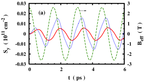
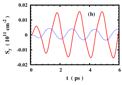
Figure 1: (Color online) (a) Spin polarization along $y$ axis, $S_{y}$, as function of time with zero initial spin polarization for $E=0.5$ kV/cm (solid curve) and 1.0 kV/cm (dotted curve). $T=50$ K and $N_{i}=0.05N_{e}$. The dashed curve is the THz-field-induced effective magnetic field $B_{\mbox{eff}}$ with $E=1.0$ kV/cm. Note that the scale of the dashed curve is on the right hand side of the frame. (b) $S_{y}$ vs. time for $E=1.0$ kV/cm with $B_{\mbox{eff}}$ included (solid curve) and excluded (dotted curve).

As pointed out after Eq. (3) that the anisotropic term $\gamma_{E}k_{x}\Omega\cos(\Omega t)$ in the Hamiltonian breaks down $k_{x}\to-k_{x}$ symmetry. However, without scattering, the density matrix in the Floquet picture does not change with time and is determined solely by its initial value. For the choice of isotropic initial distribution, the $k_{x}\to-k_{x}$ asymmetry of the density matrix never shows up. In the presence of scattering, the density matrix should show the asymmetry of the Hamiltonian. Consequently, the average of $k_{x}$ of the electron system, $\langle k_{x}\rangle$, is nonzero. Below we will show that, quite remarkably, the scattering terms within the RWA keeps the symmetry of $k_{x}\to-k_{x}$ and the scattering terms which do not keep the symmetry only appear in the time-dependent (beyond RWA) scattering terms.

Look at, e.g., the electron-impurity scattering [Eq. (12)], the weight of the $n$-th sideband-modulated scattering is $P_{n}^{(\eta\eta_{1}\eta_{2}\eta_{3})}=S^{(\eta\eta_{1})}_{{\bf k},{\bf k}^{\prime}}(t,0)S^{(n)(\eta_{2}\eta_{3})}_{{\bf k}^{\prime},{\bf k}}$. As the main source of the sideband effect is the term $\gamma_{E}k_{x}\Omega\cos(\Omega t)$ in the Hamiltonian [Eq. (3)], the weight is approximately

$$P_{n}^{(\eta\eta_{1}\eta_{2}\eta_{3})} = \delta_{\eta\eta_{1}}\delta_{\eta_{2}\eta_{3}}e^{i[(\varepsilon_{{\bf k}}-\varepsilon_{{\bf k}^{\prime}})t+\gamma_{E}\sin(\Omega t)(k_{x}-k_{x}^{\prime})]}$$ (26)

$$\mbox{}\times J_{n}[\gamma_{E}(k_{x}^{\prime}-k_{x})].$$

$P_{n}$ can be further decomposed into the time-independent $P_{n}^{in}$ and the time-dependent $P_{n}^{d}=P_{n}^{d1}+P_{n}^{d2}$ parts (omitting the superscripts of $\eta$):

$$P_{n}^{in}=J_{n}\left(\gamma_{E}(k_{x}^{\prime}-k_{x})\right)J_{n}\left(\gamma_{E}(k_{x}^{\prime}-k_{x})\right),$$ (27)

$$P_{n}^{d1} = \sum_{m:\mbox{even}\ m\neq 0}J_{n+m}\left[\gamma_{E}(k_{x}^{\prime}-k_{x})\right]$$ (28)

$$\mbox{}\times J_{n}\left[\gamma_{E}(k_{x}^{\prime}-k_{x})\right]e^{-im\Omega t},$$

$$P_{n}^{d2} = \sum_{m:\mbox{odd}}J_{n+m}\left[\gamma_{E}(k_{x}^{\prime}-k_{x})\right]$$ (29)

$$\mbox{}\times J_{n}\left[\gamma_{E}(k_{x}^{\prime}-k_{x})\right]e^{-im\Omega t}.$$

It is seen that under the transformation: $k_{x}^{\prime}\to-k_{x}^{\prime}$ and $k_{x}\to-k_{x}$, $P_{n}^{in}$ and $P_{n}^{d1}$ are invariant but $P_{n}^{d2}$ is changed. This indicates that a portion of the time-dependent (beyond RWA) scattering terms break down the $k_{x}\to-k_{x}$ symmetry. With these scattering terms, the density matrix should evolve to be asymmetric in $k_{x}$ direction. This leads to $\langle k_{x}\rangle\neq 0$. $\langle k_{x}\rangle$ should also oscillate with time as $P_{n}^{d2}$ does.

In the presence of the SOC, $\langle k_{x}\rangle$ leads to a second effective magnetic field:

$$B_{av}(t)=2\alpha_{R}\langle k_{x}\rangle/(|g|\mu_{B}).$$ (30)

Indeed, we find that the spin polarization $S_{y}$ is still nonzero when $B_{\mbox{eff}}$ is turned off by omitting the corresponding term in the Hamiltonian. In Fig. 1(b), we plot $S_{y}(t)$ for both cases with and without $B_{\mbox{eff}}$. It is seen that $S_{y}$ is nonzero when $B_{\mbox{eff}}$ is excluded, although the amplitude is reduced. This spin polarization is induced by $B_{av}$ via Pauli paramagnetism. The results indicate that $B_{av}$ oscillates with time and is smaller than $B_{\mbox{eff}}$. Moreover, there is a change in the delay of the oscillation due to different time-dependence of $B_{av}$ compared to $B_{\mbox{eff}}$. This difference also contributes to the delay of the spin polarization which is induced by the total effective magnetic field ${\cal B}$ (${\cal B}\equiv B_{\mbox{eff}}+B_{av}$).

Finally, it is found that a small initial spin polarization ($\sim 4\%$) along the $z$ axis makes marginal effect on the time dependence of $S_{y}$.

III.1.2 Steady-state spin polarization

In this subsection, we discuss the dependence of the amplitude of the steady-state spin polarization $S_{y}^{0}$ (the peak value of $S_{y}$) on the THz field.

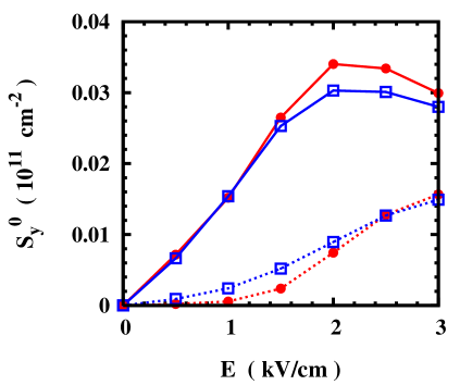
Figure 2: (Color online) Dependence of the ASSSP on THz field strength for $T=50$ K (solid curve with $\bullet$) and 100 K (solid curve with $\square$) without impurities ($N_{i}=0$). The dotted curves are the same as the solid ones but without the THz-field-induced effective magnetic field $B_{\mbox{eff}}$.

In Fig. 2 we plot the amplitude of the steady-state spin polarization (ASSSP) as a function of THz field strength for the cases with and without the THz-field-induced effective magnetic field $B_{\mbox{eff}}$. Two typical lattice temperatures $T=50$ K and $100$ K are investigated with the impurity density $N_{i}=0$. It is seen that the ASSSP first increases then decreases with the strength of the THz field. The effective magnetic field increases with the THz field strength. According to Pauli paramagnetism, however, the spin polarization should always increase with the magnetic field. Here the decrease of the ASSSP mainly originates from the hot-electron effect. To elucidate this point, we plot the hot-electron temperature $T_{e}$ in Fig. 3 (the method used to obtain $T_{e}$ is given in Appendix C). It is seen that the hot-electron temperature increases with the THz field strength. The increase of the hot-electron temperature decreases the induced spin polarization according to Pauli paramagnetism. It is noted from the figure that the largest ASSSP can be $\sim 3.5\times 10^{9}$ cm^-2 which corresponds to a large spin polarization of $7$ %. This indicates that the intense THz field is a very efficient tool in generating spin polarization. It can be noticed in Fig. 2 that the ASSSP is smaller at higher temperature. The decrease of the ASSSP is due to the increase of the hot-electron temperature with the lattice temperature, as indicated in Fig. 3.

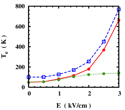
Figure 3: (Color online) Hot-electron temperature $T_{e}$ as function of THz field strength for $T=50$ K (solid curve with $\bullet$) and 100 K (dashed curve with $\square$) without impurities ($N_{i}=0$). The dotted curve with $\bullet$ is the same as the solid one, but with only $n=0,\pm 1$ allowed in the sideband-modulated scattering.

It should be pointed out that, differing from our previous study on spin relaxation in quantum dots,Jiang2 here the $n$-th sideband-modulated scattering rate differs little from each other. The energy conservation (the $\delta$ functions in the scattering terms) gives different final state for different $n$ with given initial state, thus the momentum transferred into the system can change effectively with $n$. However, the matrix elements of all the scattering mechanisms vary slowly with the momentum due to the screening and the quantum confinement along the growth direction. Consequently, the sideband-modulated scattering rate varies slowly with $n$ and the manipulation of the spin relaxation via sideband modulation of the spin-flip scattering does not apply in 2DES. In 2DES, the main effect of the sideband-modulated scattering is the hot-electron effect. As we have pointed out, the $n$-th sideband-modulated scattering tends to make the distribution be flatter in the energy range of $n\Omega$, which thus leads to the hot-electron effect. In Fig. 3, we also plot the hot-electron temperature when the summations of $n$ in the scattering terms [Eqs. (12), (13) and (14)] are restricted to $n=0,\pm 1$. In the previous studies on the effect of THz field on spin dynamics, only these processes are considered, where the THz field is weak.Ganichev1 ; Ganichev2 ; Ganichev3 It is seen that the hot-electron temperature is largely reduced by the number of sideband involved in the scattering, especially when the THz field is strong and hence the sideband-modulated scattering with $|n|>1$ is important. This confirms the important role of sideband-modulated scattering to the hot-electron effect.

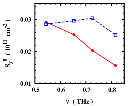
Figure 4: (Color online) Dependence of the ASSSP on THz field frequency for $E=1.5$ kV/cm ($\bullet$) and $2.5$ kV/cm ($\square$). $T=100$ K and $N_{i}=0$.

The dotted curves in Fig. 2, is the ASSSP calculated without the THz-field-induced effective magnetic field $B_{\mbox{\tiny eff}}$. As analyzed before, here the ASSSP is induced by $B_{av}$. The contribution of $B_{av}$ becomes more important when THz field strength increases. This is because that the terms $P_{n}^{d2}$ increase with the sideband effect which increases with THz field strength. Moreover, it is seen that the ASSSP due to $B_{av}$ is larger at higher temperature (100 K in the figure) when the THz field strength is small. This is because the scattering terms leading to the breakdown of $k_{x}\to-k_{x}$ symmetry increase as the electron–LO-phonon scattering is more efficient at $T=100$ K. However, when the THz field strength is larger, the hot-electron effect becomes more important. (We find that the hot-electron temperature changes little when $B_{\mbox{eff}}$ is removed.) The hot-electron effect also reduces the ASSSP induced by $B_{av}$. At large THz field strength this effect becomes more important and the difference of ASSSPs at 50 and $100$ K becomes marginal.

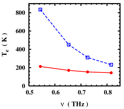
Figure 5: (Color online) Hot-electron temperature $T_{e}$ as function of the THz frequency for $E=1.5$ kV/cm ($\bullet$) and $2.5$ kV/cm ($\square$). $T=100$ K and $N_{i}=0$.

We now turn to investigate the dependence of the ASSSP on THz frequency. It is noted that the amplitude of the THz-field-induced effective magnetic field $B_{\mbox{eff}}$ [Eq. (4)] decreases with THz frequency. However, the hot-electron effect induced by the sideband effect which increases with $\gamma_{E}\Omega=eE/(m^{\ast}\Omega)$, also decreases with THz frequency. These two effects again compete with each other. In Fig. 4 we plot the ASSSP as function of the THz frequency for two cases: $E=1.5$ and $2.5$ kV/cm with $T=100$ K. It is seen that for the case with $E=2.5$ kV/cm, the ASSSP first increases then decreases with the THz frequency due to the competition of the two effects. To examine the hot-electron effect, we also plot the hot-electron temperature in Fig. 5. It is seen that the hot-electron temperature decreases with the THz frequency. For large THz frequency, the hot-electron effect is marginal and thus the ASSSP decreases with the THz frequency as the THz field induced effective magnetic field does. For smaller THz frequency the hot-electron effect becomes dominant and the ASSSP increases with the THz frequency. Consequently there is a peak frequency where the ASSSP reaches the maximum. For the case with $E=1.5$ kV/cm, there should be a peak with the peak frequency being much smaller than the frequency we calculated. This is because the hot-electron effect is much weaker than the case with $E=2.5$ kV/cm (see Fig. 5).

III.2 Spin dynamics with finite initial spin polarization

III.2.1 Temporal evolution of the spin signals

In Fig. 6, we plot the temporal evolutions of the spin signals along $z$, $x$ and $y$ axis at different THz field strengths. The initial spin polarization is taken to be 4 % along the $z$ axis. In Fig. 6(a), one finds that $S_{z}$ exhibits oscillatory decay. This resembles the low temperature spin decay observed in Refs. wu-Exp-HighP, and Harley, , which is due to the large spin-orbit effective magnetic field and weak scattering,wu-hole i.e., the system is in the weak scattering limit. It is noted that $S_{z}$ decays faster when the THz field strength increases. Moreover, the spin oscillation frequency also increases as indicated by the left-shift of the peak around 0.7 ps, which is due to the total effective magnetic field ${\cal B}$ induced by the THz field. From Fig. 6(b), one notices that a small value of $S_{x}$ is excited but eventually decays to zero. This is again due to the effective magnetic field ${\cal B}$, which rotates $S_{z}$ to $S_{x}$. The first peak value of $S_{x}$ increases with the THz field strength. Without THz field, $S_{x}\equiv 0$. In Fig. 6(c), it is seen that $S_{y}$ is also induced and reaches a non-vanishing oscillatory value after $\sim 3$ ps evolution, similar to what observed in Fig. 1 where the initial spin polarization is zero.

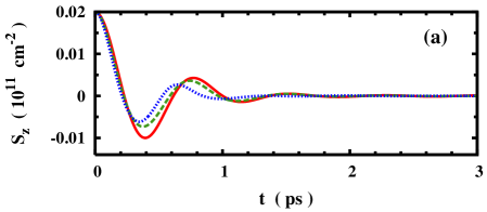
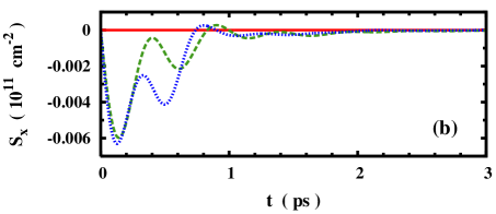
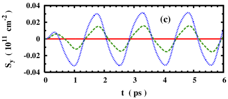
Figure 6: (Color online) Temporal evolution of the spin signals (a): $S_{z}$; (b): $S_{x}$; and (c): $S_{y}$ for THz field strengthes: 0 kV/cm (solid curves), 1 kV/cm (dashed curves), and 2 kV/cm (dotted curves). $N_{i}=0.05N_{e}$ and $T=50$ K.

III.2.2 SRT

In Fig. 7, the SRT, which is extracted via fitting the exponential decay of the envelop of $S_{z}$, is plotted as function of THz field strength for different impurity densities $N_{i}=0$, $0.02N_{e}$, and $0.05N_{e}$, with lattice temperature $T=50$ K.

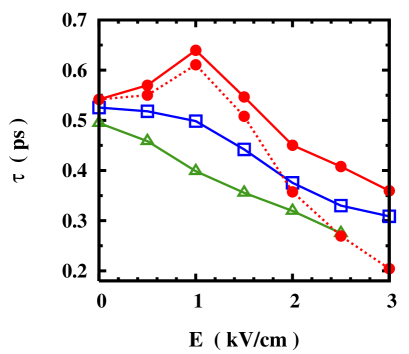
Figure 7: (Color online) Dependence of the SRT $\tau$ on THz field strength for impurity densities: $N_{i}=0$ ($\bullet$); $N_{i}=0.02N_{e}$ ($\square$); $N_{i}=0.05N_{e}$ ($\triangle$). Solid curves: from full calculation; Dotted curve: from the calculation without the THz-field-induced effective magnetic field $B_{\mbox{eff}}$.

We first discuss the case with $N_{i}$=0 (solid curve with $\bullet$). It is noted that the SRT first increases then decreases with the THz field strength. The underlying physics is that there are two consequences of the THz field: (i) the total THz field-induced effective magnetic field ${\cal B}$; (ii) the hot-electron effect. Effect (i) can give a magnetic field as large as several Tesla (2.6 T per 1 kV/cm THz field with $\nu=0.65$ THz, of which the corresponding Zeeman splitting is as large as 2.2 meV). This effective magnetic field blocks the inhomogeneous broadening from the Rashba SOC. It thus elongates the SRT.opt-or ; wu-later The main consequences of effect (ii) are the enhancement of momentum scattering as well as the inhomogeneous broadening as the electrons distribute on larger ${\bf k}$ states where the SOC is larger. Enhancement of the inhomogeneous broadening shortens the SRT according to our previous studies.wu-later ; wu-hole ; wu-lowT It is found that in the strong scattering limit, SRT increases with the momentum scattering.opt-or ; wu-review However, it is demonstrated in Ref. wu-hole, that in the weak or intermediate scattering limit, the SRT decreases with increasing the momentum scattering. In our case, due to the large Rashba SOC parameter, the system is in the weak/intermediate scattering regime. This can be further checked by the fact that the SRT decreases when the electron-impurity scattering is strengthened by increasing the impurity density, as shown in Figs. 7 and 8. Thus, effect (ii) shortens the SRT. The two effects compete with each other and hence the SRT varies non-monotonically with the THz field strength: For small THz field strength the increase of the total THz field-induced effective magnetic field ${\cal B}$ is dominant. As a result, the SRT increases; For large field strength, the hot-electron effect becomes more important. Consequently the SRT decreases.

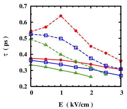
Figure 8: (Color online) Dependence of the SRT $\tau$ on THz field strength for impurity densities: $N_{i}=0$ ($\bullet$); $N_{i}=0.02N_{e}$ ($\square$); and $N_{i}=0.05N_{e}$ ($\triangle$). $T=100$ K (solid curves) and $50$ K (dashed curves).

To further elucidate the influence of effect (i), we remove part of the THz field-induced effective magnetic field, $B_{\mbox{eff}}$, by excluding the term $\alpha_{R}\hat{\sigma}_{y}eE\cos(\Omega t)/\Omega$ from the Hamiltonian, and then calculate the SRT. We plot the obtained SRT as dotted curve in Fig. 7. It is seen that the SRT is reduced, especially at large THz field strength. It is checked that the hot-electron effect changes little when $B_{\mbox{eff}}$ is removed as it is not the main source of the hot-electron effect. The results confirm that the THz field-induced effective magnetic field indeed increases the SRT.

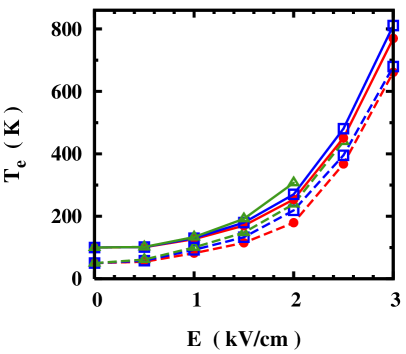
Figure 9: (Color online) Dependence of the hot-electron temperature $T_{e}$ on THz field strength for different impurity densities: $N_{i}=0$ ($\bullet$ ); $N_{i}=0.02N_{e}$ ($\square$); $N_{i}=0.05N_{e}$ ($\triangle$). $T=100$ K (solid curves) and $T=50$ K (dashed curves).

For the cases with $N_{i}=0.02N_{e}$ and $0.05N_{e}$, the SRT decreases with the THz field strength monotonically. It is noted in Fig. 9 (solid curves) that the hot-electron temperature is larger at higher impurity density. The enhancement of the hot-electron effect overcomes the increase of the effect of the THz field-induced effective magnetic field in these two cases, which leads to the monotonic decrease of the SRT.

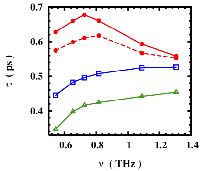
Figure 10: (Color online) Dependence of the SRT $\tau$ on THz frequency for impurity densities: $N_{i}=0$ ($\bullet$); $N_{i}=0.02N_{e}$ ($\square$); and $N_{i}=0.05N_{e}$ ($\triangle$). Solid curves: from full calculation; Dotted curve: from the calculation without the THz-field-induced effective magnetic field $B_{\mbox{eff}}$. $E=1$ kV/cm and $T=50$ K.

It should be mentioned that in the case of static electric field, the hot-electron effect is more important at smaller impurity density under a given electric field.Lei1 ; wu-hot-e ; wu-lowT However, under intense THz field the hot-electron effect is more pronounced at larger impurity density where the sideband-modulated scattering, which can transfer the THz photon energy into electron system, is stronger. Similar effects have been reported by Lei in the study of charge transport under intense THz field.Lei2

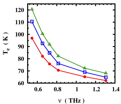
Figure 11: (Color online) Dependence of the hot-electron temperature $T_{e}$ on THz frequency for impurity densities: $N_{i}=0$ ($\bullet$); $N_{i}=0.02N_{e}$ ($\square$); and $N_{i}=0.05N_{e}$ ($\triangle$). $E=1$ kV/cm and $T=50$ K.

We further discuss the temperature dependence of the SRT. In Fig. 8 we plot the SRT as function of THz field strength at $T=100$ K and $50$ K. One can see that the SRT at high temperature ($T=100$ K) is much smaller than that at low temperature ($T=50$ K). This is because the electron–LO-phonon scattering at high temperature is much more efficient than that at low temperature. The increase of scattering thus enhances the hot-electron effect (see Fig. 9) and the enhancement of the hot-electron effect reduces the SRT. It is also noted that for all three impurity densities at $100$ K, the SRTs decrease with the THz field strength monotonically. This indicates that the hot-electron effect of the THz field is dominant as the momentum scattering is strong.

We now turn to the THz frequency dependence of the SRT. As has been demonstrated before, both the THz field-induced effective magnetic field and the hot-electron effect decrease with the increase of the THz frequency and they compete with each other on spin relaxation. In Fig. 10, we plot the SRT as function of the THz frequency for three different impurity densities: $N_{i}=0$, $0.02N_{e}$, and $0.05N_{e}$. The lattice temperature is $T=50$ K. It is noted that for the impurity-free case, the SRT first increases then decreases with the THz frequency, which is similar to the dependence of the SRT on the THz field strength. This is again due to the competition between the hot-electron effect and the THz field-induced effective magnetic field. Similarly, for the cases with $N_{i}=0.02N_{e}$ and $0.05N_{e}$, the SRT increases monotonically with the THz frequency. When $B_{\mbox{eff}}$ is removed, the SRT for impurity-free case is reduced and the peak frequency where the SRT gets maximum becomes larger. This indicates the weakening of the THz field-induced effective magnetic field since the hot-electron effect changes little.

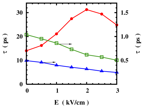
Figure 12: (Color online) Dependence of the SRT $\tau$ on THz field strength for different SOC parameters: $\alpha_{R}=1$ meV$\cdot$nm ($\bullet$); $\alpha_{R}=10$ meV$\cdot$nm ($\square$); and $\alpha_{R}=30$ meV$\cdot$nm ($\triangle$). $T=50$ K and $N_{i}=0.05N_{e}$. Note that the scale for the curves with $\square$ and $\triangle$ are on the right hand side of the frame.

Finally, we discuss the dependence of the SRT on the Rashba SOC parameter. In Fig. 12 we plot the SRT as function of THz field strength at different Rashba parameters, $\alpha_{R}=1$, 10, and 30 meV$\cdot$nm. The lattice temperature is taken to be $T=50$ K and the impurity density is $N_{i}=0.05N_{e}$. It is seen that for small Rashba SOC coefficient $\alpha_{R}=1$ meV$\cdot$nm, the SRT first increases then decreases with the THz field strength. However, for large SOC, the SRT decreases monotonically with the THz field strength. As has been revealed previously that in the presence of the impurity density $N_{i}=0.05N_{e}$, the hot-electron effect dominates the SRT. The hot-electron effect leads to the increase of both the scattering and the inhomogeneous broadening. For the case with $\alpha_{R}=1$ meV$\cdot$nm, which is in the strong scattering regime, increase of scattering leads to longer SRT; whereas the increase of inhomogeneous broadening leads to shorter SRT. Therefore, the two effects compete with each other: the SRT first increases due to the enhancement of scattering and then decreases due to the increase of inhomogeneous broadening. This behavior is similar to the case under a strong static electric field.wu-hot-e For the cases with larger SOC, which is in the intermediate scattering regime, both effects decrease the SRT.

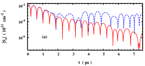
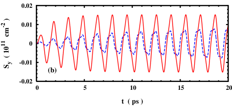
Figure 13: (Color online) Temporal evolution of the spin signals calculated with the electron–electron scattering is included (solid curve) and excluded (dashed curve). (a): $|S_{z}|$; (b): $S_{y}$. $E=1$ kV/cm, $T=50$ K and $N_{i}=0$.

III.3 Effect of electron-electron Coulomb scattering

Previously it has been shown that the electron-electron Coulomb scattering plays an important role in spin relaxation due to the DP mechanism.wu-early ; wu-hot-e ; wu-helix ; wu-lowT ; wu-hole ; Ivchenko ; Ji Furthermore, for systems under strong electric field, the electron-electron Coulomb scattering is crucial for the electron system to establish its quasi-equilibrium state.wu-hot-e Here we demonstrate that it also has nontrivial effects on the spin dynamics under intense THz field. In Fig. 13, we plot the temporal evolution of the spin signals, $|S_{z}|$ and $S_{y}$, calculated with the electron-electron scattering included (solid curve) and excluded (dashed curve) under same initial distributions and conditions. It is seen from Fig. 13(a) that in the case with the electron-electron Coulomb scattering, $|S_{z}|$ exhibits good exponential decay, superimposed by the THz oscillations. Otherwise, the decay is non-exponential and the decay rate becomes much slower, which indicates that the spin relaxation is markedly reduced. It is further seen from Fig. 13(b) that with electron-electron Coulomb scattering, $S_{y}$ reaches the steady state much faster with a larger peak value. All these demonstrate the importance of the electron-electron Coulomb scattering to the spin dynamics.

IV Conclusion and discussion

IV.1 Conclusion

In conclusion, we have developed the kinetic spin Bloch equations for 2DES with Rashba SOC under intense THz laser fields, with all the relevant scattering mechanisms such as the electron-impurity, electron-phonon and electron-electron Coulomb scattering explicitly included. The formalism is very general and can be applied to study spin kinetics in many-body electron or hole system under strong time-periodic driving fields with arbitrary SOC. Moreover, our formalism goes beyond the RWA treatment of the scattering. By solving the kinetic spin Bloch equations numerically, we investigate the effect of the intense THz fields on the spin kinetics. We focus on the THz field-induced steady-state spin polarization and the effect of the THz field on spin relaxation.

We first study the temporal evolution of the spin polarization under intense THz field at zero initial spin polarization. We find that the THz field can pump a finite steady-state THz spin polarization in the presence of all relevant scattering. The spin polarization is induced by the THz field-induced effective magnetic field in the presence of SOC. The maximum spin polarization in the steady state can be as large as 7 %, which shows that the intense THz field is a very efficient tool in generating spin polarization.

As our approach goes beyond the RWA treatment of the scattering, we find some interesting features which are absent in the RWA treatment. The first feature is that there is always a retardation of the spin polarization in response to the THz field-induced effective magnetic field. Another feature is that, as the Hamiltonian breaks the $k_{x}\to-k_{x}$ symmetry via the term $\gamma_{E}k_{x}\Omega\cos(\Omega t)$, the average of $k_{x}$ over the electron system $\langle k_{x}\rangle$ becomes nonzero and oscillates with time. In the presence of SOC, $\langle k_{x}\rangle$ leads to another effective magnetic field which also induces spin polarization. We find that, remarkably, under the RWA, the $k_{x}\to-k_{x}$ symmetry is still kept.

We further study the dependence of the amplitude of the steady-state spin polarization on the THz field for different lattice temperatures, impurity densities and Rashba SOC parameters. It is found that the main consequences of the THz field are: (i) the hot-electron effect due to sideband-modulated scattering and (ii) the THz field-induced effective magnetic field due to the SOC. Both effects increase with the THz field strength but decrease with the THz frequency. The amplitude of the steady-state spin polarization increases with effect (ii), but decreases with effect (i) according to the Pauli paramagnetism. At small THz field strength (and/or large THz frequency) the hot-electron effect is weak and effect (ii) dominates. The amplitude of the steady-state spin polarization thus increases (decreases) with the field strength (frequency). At large THz field strength (low THz frequency), the hot-electron effect becomes more important than effect (ii) and the amplitude of the steady-state spin polarization decreases (increases) with the THz field strength (frequency).

We also find that the THz field can strongly change the SRT due to the two effects addressed above. Specifically, the hot-electron effect shortens the SRT via enhancement of momentum scattering and inhomogeneous broadening for the system in weak/intermediate scattering limit. Meanwhile, effect (ii) increases the SRT due to the blocking of the inhomogeneous broadening. For small impurity densities at low temperature, when the THz field strength is small (and/or the THz frequency is large), the hot-electron effect is weak, and effect (ii) becomes dominant. The SRT thus increases (decreases) with the THz field strength (frequency). At large THz field strength (small THz frequency) the hot-electron effect is more important than effect (ii). The SRT thus decreases (increases) with the THz field strength (frequency). However, for large impurity densities or high temperatures, the enhancement of the hot-electron effect overcomes the increase of the effect (ii). Consequently the SRT decreases (increases) with the THz field strength (frequency). We also discuss the SOC dependence of the SRT at large impurity densities where the hot-electron effect dominates. For small SOC, which is in the strong scattering regime, the SRT first increases with the THz field strength due to enhancement of momentum scattering, then decreases with it due to enhancement of the inhomogeneous broadening. For large SOC, which is in the weak/intermediate scattering regime, increase of scattering also reduces the SRT. Consequently, the SRT decreases monotonically with the THz field strength.

IV.2 Discussion

Finally we compare our study with the electric dipole spin resonance (EDSR) in the literature. To simplify the discussion, we introduce a simple spin Hamiltonian which characterize the spin dynamics of our Hamiltonian [Eq. (3)] and the EDSR:

$$\hat{H}_{spin}(t)=\frac{1}{2}(\Delta_{0}+\Delta_{1})\hat{\sigma}_{x}+\frac{1}{2}\Delta_{2}\hat{\sigma}_{y}+\gamma\cos(\Omega t)\hat{\sigma}_{y}.$$ (31)

Here $\Delta_{1}$ and $\Delta_{2}$ characterize the ${\bf k}$-dependent effective magnetic fields due to the SOC. $\Delta_{0}$ represents the external static magnetic field used in the EDSR set-up.Rashba0 ; Rashba1 ; Rashba2 ; Rashba3 ; Duckheim (For our case: $\Delta_{0}=0$, $\Delta_{1}=2\alpha_{R}k_{y}$, $\Delta_{2}=-2\alpha_{R}k_{x}$, $\gamma=-\alpha_{R}eE/\Omega$.) In EDSR, $\Delta_{0}$ is usually much larger than $\Delta_{1}$, $\Delta_{2}$ and $\gamma$, and $\Delta_{0}=\Omega$.Kato1 ; Meier To the lowest order approximation, the spin dynamics is governed by $H^{0}_{spin}=\frac{1}{2}\Delta_{0}\hat{\sigma}_{x}+\gamma\cos(\Omega t)\hat{\sigma}_{y}$. In the RWA the solutions of the Schödinger equation are given by $\Psi_{\pm}=e^{\pm i\gamma t}\frac{1}{\sqrt{2}}(e^{-i\Omega t/2}\chi_{+}\pm ie^{i\Omega t/2}\chi_{-})$ with $\hat{\sigma}_{x}\chi_{\pm}=\pm\chi_{\pm}$. With initial condition $\psi=\chi_{+}$, one obtains $\langle S_{x}\rangle=\frac{1}{2}\cos(\gamma t)$, which is the well-known Rabi oscillation. The ${\bf k}$-dependent $\Delta_{1}$ and $\Delta_{2}$ effective magnetic fields lead to the damping of the Rabi oscillation due to the DP mechanism in the presence of scattering.Duckheim For the case of strong driving field ($\gamma\gtrsim\Omega$), the solutions of the Schödinger equation are the Floquet wave functions $\Psi_{{\bf k}\eta}$ given in Eq. (6). Now the spin dynamics is given by

$$\langle S_{i}\rangle = \sum_{{\bf k};\eta,\eta^{\prime};n,m;\sigma,\sigma^{\prime}}\rho^{F(\eta^{\prime}\eta)}_{\bf k}\upsilon_{n\sigma}^{{\bf k}\eta\ast}\upsilon_{m\sigma^{\prime}}^{{\bf k}\eta^{\prime}}\langle\sigma|\frac{1}{2}\hat{\sigma}_{i}|\sigma^{\prime}\rangle$$ (32)

$$\mbox{}\times e^{it[y_{{\bf k}\eta}-y_{{\bf k}\eta^{\prime}}+(m-n)\Omega]},$$

with $i=x,y,z$. From the above equation, it is seen that, unlike the weak driving-field case where only a single Rabi frequency is observable, here the spin signal $S_{i}(t)$ oscillates at many frequencies $y_{{\bf k}\eta}-y_{{\bf k}\eta^{\prime}}+(m-n)\Omega$ (with $m-n=0,\pm 1,\pm 2,\cdots$). Moreover, in our case, $\Delta_{1}$, $\Delta_{2}$, $\gamma$ and $\Omega$ are on the same order of magnitude while $\Delta_{0}=0$. Thus the spin precession frequency varies largely with ${\bf k}$. This large inhomogeneous broadening of spin precession frequency smears out the driving field-induced Rabi oscillation of the spin polarization signals.

Appendix A Derivation of electron-impurity scattering term in Floquet-Markov limit

Here we give terms due to electron-impurity scattering as an example. Terms due to other scattering can be obtained similarly. From nonequilibrium Green function theory,Haugbook the electron-impurity scattering term can be written as

$$\left.\partial_{t}\rho_{{\bf k}}\right|_{ei}=\Big{\{}-{\cal{A}}^{ei}_{{\bf k}}(><)+{\cal{A}}^{ei}_{{\bf k}}(<>)\Big{\}}+\Big{\{}...\Big{\}}^{\dagger},$$ (33)

where

$${\cal{A}}^{ei}_{{\bf k}}(><)=\sum_{{\bf k}^{\prime},q_{z}}n_{i}U_{{\bf k}-{\bf k}^{\prime},q_{z}}^{2}|I(iq_{z})|^{2}$$

$$\mbox{}\times\int_{-\infty}^{t}\!\!d{\tau}\hat{U}_{0}^{e}({\bf k}^{\prime},t,\tau)\hat{\rho}^{>}_{{\bf k}^{\prime}}(\tau)\hat{\rho}^{<}_{\bf k}(\tau)\hat{U}_{0}^{e}({\bf k},\tau,t).$$ (34)

${\cal{A}}^{ei}_{{\bf k}}(<>)$ can be obtained by interchanging $>$ and $<$. It is better to work in the interaction picture, or the “Floquet picture”:

$$\hat{\rho}^{\gtrless F}_{\bf k}(t)=\hat{U}_{0}^{e\ \dagger}({\bf k},t,0)\hat{\rho}^{\gtrless}_{\bf k}(t)\hat{U}_{0}^{e}({\bf k},t,0).$$ (35)

After this transformation, the term becomes

$${\tilde{\cal{A}}^{ei}}_{{\bf k}}(><) = \hat{U}_{0}^{e\ \dagger}({\bf k},t,0){\cal{A}}^{ei}_{{\bf k}}(><)\hat{U}_{0}^{e}({\bf k},t,0)$$ (36)

$$= \sum_{{\bf k}^{\prime},q_{z}}n_{i}U_{{\bf k}-{\bf k}^{\prime},q_{z}}^{2}|I(iq_{z})|^{2}\int_{-\infty}^{t}\!\!d{\tau}\hat{S}_{{\bf k},{\bf k}^{\prime}}(t,0)$$

$$\mbox{}\times\hat{\rho}^{>F}_{{\bf k}^{\prime}}(\tau)\hat{S}_{{\bf k}^{\prime},{\bf k}}(\tau,0)\hat{\rho}^{<F}_{\bf k}(\tau),$$

where $\hat{S}_{{\bf k},{\bf k}^{\prime}}(t,0)=\hat{U}_{0}^{e\ \dagger}({\bf k},t,0)\hat{U}_{0}^{e}({\bf k}^{\prime},t,0)$. According to Floquet-Markov theory, the Markov approximation should be made with respect to the spectrum determined by the Floquet wavefunctions, i.e., $\hat{\rho}^{\gtrless F}_{\bf k}(\tau)\approx\hat{\rho}^{\gtrless F}_{\bf k}(t)$. Thus, the scattering term becomes

$${\tilde{\cal{A}}^{ei}}_{{\bf k}}(><) = \sum_{{\bf k}^{\prime},q_{z}}n_{i}U_{{\bf k}-{\bf k}^{\prime},q_{z}}^{2}|I(iq_{z})|^{2}\hat{S}_{{\bf k},{\bf k}^{\prime}}(t,0)$$ (37)

$$\mbox{}\times\hat{\rho}^{>F}_{{\bf k}^{\prime}}(t)\int_{-\infty}^{t}\!\!d{\tau}\hat{S}_{{\bf k}^{\prime},{\bf k}}(\tau,0)\hat{\rho}^{<F}_{\bf k}(t).$$

The next step toward the explicit form of the scattering term is based on the analysis of the elements of $\hat{S}$. Expanding the kinetic equations in the basis of {$|\xi_{{\bf k}\eta}(0)\rangle$}, the elements of $\hat{S}$ are given by

$$S^{(\eta_{1}\eta_{2})}_{{\bf k}^{\prime},{\bf k}}(t,0) = \langle\xi_{{\bf k}^{\prime}\eta_{1}}(t)|\xi_{{\bf k}\eta_{2}}(t)\rangle$$ (38)

$$\mbox{}\times e^{i[(\varepsilon_{{\bf k}^{\prime}}-\varepsilon_{\bf k})t+\gamma_{E}\sin(\Omega t)(k_{x}^{\prime}-k_{x})]}$$

$$= \sum_{n}S^{(n)(\eta_{1}\eta_{2})}_{{\bf k}^{\prime},{\bf k}}e^{it(n\Omega+\bar{\varepsilon}_{{\bf k}^{\prime}\eta_{1}}-\bar{\varepsilon}_{{\bf k}\eta_{2}})}.$$

The scattering term can then be explicitly laid out by expanding all the operators in the basis of {$|\xi_{{\bf k}\eta}(0)\rangle$}:

$$\hskip 4.26773pt{\tilde{\cal{A}}^{ei}}_{{\bf k}}(><)|^{(\eta\eta^{\prime})} = \sum_{{\bf k}^{\prime},q_{z},n,\eta_{1}\eta_{2}\eta_{3}}\pi n_{i}U_{{\bf k}-{\bf k}^{\prime},q_{z}}^{2}|I(iq_{z})|^{2}$$ (39)

$$\mbox{}\times S^{(\eta\eta_{1})}_{{\bf k},{\bf k}^{\prime}}(t,0)\rho^{>F(\eta_{1}\eta_{2})}_{{\bf k}^{\prime}}(t)S^{(n)(\eta_{2}\eta_{3})}_{{\bf k}^{\prime},{\bf k}}\rho^{<F(\eta_{3}\eta^{\prime})}_{\bf k}(t)$$

$$\mbox{}\times\delta(n\Omega+\bar{\varepsilon}_{{\bf k}^{\prime}\eta_{2}}-\bar{\varepsilon}_{{\bf k}\eta_{3}}).$$

According to Eq. (A1), one can readily arrive at the full expression of the electron-impurity scattering term, which is exactly Eq. (12).

Appendix B Numerical scheme

Our numerical scheme is based on the scheme laid out in detail in Ref. wu-hot-e, , where the nonlinear kinetic spin Bloch equations are solved self-consistently with high accuracy.wu-later ; wu-lowT ; wu-Exp-HighP ; wu-Exp-Aniso The scheme is based on a discretization of the two dimensional momentum space with $N\times M$ control regions where the ${\bf k}$-grid points are chosen to be ${\bf k}_{l,m}=\sqrt{2m^{\ast}E_{l}}(\cos\theta_{m},\sin\theta_{m})$. In principle, the coherent terms are easily solved. However, the scattering terms are difficult to solve as the $\delta$-functions are hard to be integrated numerically. To facilitate the evaluation of the $\delta$-functions in the scattering terms, we set $E_{l}=(l+1/2)\Delta E$ and $\omega_{LO}=n_{LO}\Delta E$ where $l$ and $n_{LO}$ are integer numbers and $\Delta E$ is the energy span in each control region.wu-hot-e To apply this scheme to the kinetic spin Bloch equations with THz field, we also set $\Omega=n_{\mbox{\tiny THz}}\Delta E$ with $n_{\mbox{\tiny THz}}$ being integer number (typically $1\sim 3$ in our calculation). However, the $\delta$-functions are still difficult to be evaluated as $y_{{\bf k}\eta}$ and $\Delta E$ are not commensurable. We therefore use the approximation $y_{{\bf k}\eta}\approx N^{y}_{{\bf k}\eta}\Delta E$, with $N^{y}_{{\bf k}\eta}$ being the integer part of $y_{{\bf k}\eta}/\Delta E$. This approximation affects the spin kinetics marginally as $|y_{{\bf k}\eta}-N^{y}_{{\bf k}\eta}\Delta E|$ is usually much smaller than $k_{B}T$ and/or the chemical potential. Moreover, as the driving field is very strong, the spectrum of the Floquet states is mainly determined by the sideband effect and $y_{{\bf k}\eta}-N^{y}_{{\bf k}\eta}\Delta E$ only plays a quite marginal role. Furthermore, one can approach the exact results by increasing $n_{\mbox{\tiny THz}}$. In our computation, we make sure that for $n_{\mbox{\tiny THz}}$ we choose, the relative error is less than $5$ %. To make the treatment consistent, we also approximate $S^{(\eta_{1}\eta_{2})}_{{\bf k}^{\prime},{\bf k}}(t,0)\approx\sum_{n}S^{(n)(\eta_{1}\eta_{2})}_{{\bf k}^{\prime},{\bf k}}e^{it[n\Omega+\varepsilon_{{\bf k}^{\prime}}-\varepsilon_{\bf k}+(N^{y}_{{\bf k}^{\prime}\eta_{1}}-N^{y}_{{\bf k}\eta_{2}})\Delta E]}$. Or more concisely, $\hat{S}_{{\bf k}^{\prime},{\bf k}}(t,0)\approx\sum_{n}\hat{{\cal{R}}}^{(n)}_{{\bf k}^{\prime},{\bf k}}e^{it(n\Delta E+\varepsilon_{{\bf k}^{\prime}}-\varepsilon_{\bf k})}=\hat{{\cal{R}}}_{{\bf k}^{\prime},{\bf k}}(t,0)$, where ${\cal{R}}^{(n)(\eta_{1}\eta_{2})}_{{\bf k}^{\prime},{\bf k}}=S^{(m)(\eta_{1}\eta_{2})}_{{\bf k}^{\prime},{\bf k}}$ with $m$ satisfying $mn_{\mbox{\tiny THz}}+N^{y}_{{\bf k}^{\prime}\eta_{1}}-N^{y}_{{\bf k}\eta_{2}}=n$. Correspondingly, $\hat{T}_{{\bf k}^{\prime},{\bf k}}(t,0)\approx\sum_{n}\hat{{\cal{W}}}^{(n)}_{{\bf k}^{\prime},{\bf k}}e^{it(n\Delta E+\varepsilon_{{\bf k}^{\prime}}-\varepsilon_{\bf k})}=\hat{{\cal{W}}}_{{\bf k}^{\prime},{\bf k}}(t,0)$, with ${\cal{W}}^{(n)(\eta_{1}\eta_{2})}_{{\bf k}^{\prime},{\bf k}}=T^{(m)(\eta_{1}\eta_{2})}_{{\bf k}^{\prime},{\bf k}}$. We keep the coherent precession due to $y_{{\bf k}\eta}-N^{y}_{{\bf k}\eta}\Delta E$ by adding it into the coherent term. After these approximations, the coherent and scattering terms of the kinetic spin Bloch equations read

$$\left.\partial_{t}\hat{\rho}^{F}_{{\bf k}}(t)\right|_{coh}=i\Big{[}\sum_{{\bf k}^{\prime},q_{z},n}V_{{\bf k}-{\bf k}^{\prime},q_{z}}|I(iq_{z})|^{2}\hat{{\cal{W}}}_{{\bf k},{\bf k}^{\prime}}(t,0)\hat{\rho}^{F}_{{\bf k}^{\prime}}(t)$$

$$\hskip 39.83368pt\mbox{}\times\hat{{\cal{W}}}_{{\bf k}^{\prime},{\bf k}}(t,0)-\hat{H}_{r}({\bf k}),\ \hat{\rho}^{F}_{{\bf k}}(t)\Big{]},$$ (40)

with $H_{r}({\bf k})^{\eta_{1},\eta_{2}}=\delta_{\eta_{1},\eta_{2}}(y_{{\bf k}\eta_{1}}-N^{y}_{{\bf k}\eta_{1}}\Delta E)$,

$$\left.\partial_{t}\hat{\rho}^{F}_{{\bf k}}(t)\right|_{ei} = -\sum_{{\bf k}^{\prime},n,q_{z}}\pi n_{i}U^{2}_{{\bf k}-{\bf k}^{\prime},q_{z}}|I(iq_{z})|^{2}$$ (41)

$$\mbox{}\times\delta(n\Delta E+\varepsilon_{{\bf k}^{\prime}}-\varepsilon_{\bf k})\bigg{[}\Big{\{}\hat{{\cal{R}}}_{{\bf k},{\bf k}^{\prime}}(t,0)\hat{{\cal{R}}}^{(n)}_{{\bf k}^{\prime},{\bf k}}\hat{\rho}^{F}_{\bf k}(t)$$

$$\mbox{}-\hat{{\cal{R}}}_{{\bf k},{\bf k}^{\prime}}(t,0)\hat{\rho}^{F}_{{\bf k}^{\prime}}(t)\hat{{\cal{R}}}^{(n)}_{{\bf k}^{\prime},{\bf k}}\Big{\}}\ +\Big{\{}...\Big{\}}^{\dagger}\bigg{]},$$

$$\left.\partial_{t}\hat{\rho}^{F}_{{\bf k}}(t)\right|_{ep} = -\sum_{{\bf k}^{\prime},n,\lambda,\pm,q_{z}}\pi|M_{\lambda,{\bf k}-{\bf k}^{\prime},q_{z}}|^{2}|I(iq_{z})|^{2}$$ (42)

$$\mbox{}\times\delta(\pm\omega_{\lambda,{\bf k}-{\bf k}^{\prime},q_{z}}+n\Delta E+\varepsilon_{{\bf k}^{\prime}}-\varepsilon_{\bf k})e^{\mp it\omega_{\lambda,{\bf k}-{\bf k}^{\prime},q_{z}}}$$

$$\mbox{}\times\bigg{[}\Big{\{}N^{\pm}_{\lambda,{\bf k}-{\bf k}^{\prime},q_{z}}\hat{{\cal{R}}}_{{\bf k},{\bf k}^{\prime}}(t,0)\big{(}\hat{1}-\hat{\rho}^{F}_{{\bf k}^{\prime}}(t)\big{)}\hat{{\cal{R}}}^{(n)}_{{\bf k}^{\prime},{\bf k}}\hat{\rho}^{F}_{\bf k}(t)$$

$$\mbox{}-\hat{{\cal{R}}}_{{\bf k},{\bf k}^{\prime}}(t,0)\hat{\rho}^{F}_{{\bf k}^{\prime}}(t)\hat{{\cal{R}}}^{(n)}_{{\bf k}^{\prime},{\bf k}}\big{(}\hat{1}-\hat{\rho}^{F}_{{\bf k}}(t)\big{)}\Big{\}}+\Big{\{}...\Big{\}}^{\dagger}\bigg{]},$$

$$\left.\partial_{t}\hat{\rho}^{F}_{{\bf k}}(t)\right|_{ee} = -\sum_{{\bf k}^{\prime},{\bf k}^{\prime\prime},n,n^{\prime}}\pi\Big{[}\sum_{q_{z}}V_{{\bf k}-{\bf k}^{\prime},q_{z}}|I(iq_{z})|^{2}\Big{]}^{2}$$ (43)

$$\mbox{}\times\delta(n\Delta E+\varepsilon_{{\bf k}^{\prime}}-\varepsilon_{\bf k}+\varepsilon_{{\bf k}^{\prime\prime}}-\varepsilon_{{\bf k}^{\prime\prime}-{\bf k}+{\bf k}^{\prime}})$$

$$\mbox{}\times\bigg{[}\Big{\{}\hat{{\cal{W}}}_{{\bf k},{\bf k}^{\prime}}(t,0)\big{(}\hat{1}-\hat{\rho}^{F}_{{\bf k}^{\prime}}(t)\big{)}\hat{{\cal{W}}}^{(n^{\prime})}_{{\bf k}^{\prime},{\bf k}}\hat{\rho}^{F}_{\bf k}(t)$$

$$\mbox{}\times\mbox{Tr}\big{[}\hat{{\cal{W}}}^{(n-n^{\prime})}_{{\bf k}^{\prime\prime},{\bf k}^{\prime\prime}-{\bf k}+{\bf k}^{\prime}}\hat{\rho}^{F}_{{\bf k}^{\prime\prime}-{\bf k}+{\bf k}^{\prime}}(t)\hat{{\cal{W}}}_{{\bf k}^{\prime\prime}-{\bf k}+{\bf k}^{\prime},{\bf k}^{\prime\prime}}(t,0)$$

$$\mbox{}\times\big{(}\hat{1}-\hat{\rho}^{F}_{{\bf k}^{\prime\prime}}(t)\big{)}\big{]}\ -\ \hat{{\cal{W}}}_{{\bf k},{\bf k}^{\prime}}(t,0)\hat{\rho}^{F}_{{\bf k}^{\prime}}(t)\hat{{\cal{W}}}^{(n^{\prime})}_{{\bf k}^{\prime},{\bf k}}$$

$$\mbox{}\times\big{(}\hat{1}-\hat{\rho}^{F}_{\bf k}(t)\big{)}\mbox{Tr}\big{[}\hat{{\cal{W}}}^{(n-n^{\prime})}_{{\bf k}^{\prime\prime},{\bf k}^{\prime\prime}-{\bf k}+{\bf k}^{\prime}}\big{(}\hat{1}-\hat{\rho}^{F}_{{\bf k}^{\prime\prime}-{\bf k}+{\bf k}^{\prime}}(t)\big{)}$$

$$\mbox{}\times\hat{{\cal{W}}}_{{\bf k}^{\prime\prime}-{\bf k}+{\bf k}^{\prime},{\bf k}^{\prime\prime}}(t,0)\hat{\rho}^{F}_{{\bf k}^{\prime\prime}}(t)\big{]}\Big{\}}+\Big{\{}...\Big{\}}^{\dagger}\bigg{]}.$$

Now, the kinetic spin Bloch equations can be treated via the numerical scheme in Ref. wu-hot-e, . The only difference is the summations over sideband indexes which increase the complexity of the calculation. Typically, the sideband index runs through $[-24,24]$ ($[-3,3]$) for the electron-impurity and electron-phonon scattering (the electron-electron Coulomb scattering) to converge the results when the THz field is $E=1.5$ kV/cm with $\nu=0.65$ THz.

As mentioned in Sec. III, the initial distribution of the electron system is chosen to be a spin polarized hot-electron distribution under the THz field, which is obtained by sufficient long time (typically $\sim 10$ ps) evolution from a spin-polarized Fermi distribution at the lattice temperature with the SOC being turned off.wu-hot-e In Fig. 14, we plot the time evolution of the distribution on the two Floquet states with ${\bf k}=(1.1k_{F}^{0},0)$ ($k_{F}^{0}$ is the Fermi wave vector): $\rho_{\bf k}^{F(--)}$ (solid curve) and $\rho_{\bf k}^{F(++)}$ (dotted curve) for the case with 4 % initial spin polarization along the $z$ axis.

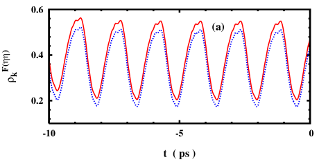
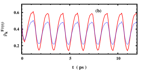
Figure 14: (Color online) Time evolution of the distribution of two Floquet states with ${\bf k}=(1.1k_{F}^{0},0)$: $\rho_{\bf k}^{F(--)}$ (solid curve) and $\rho_{\bf k}^{F(++)}$ (dotted curve). (a): initial distribution preparation without the SOC; (b): after the preparation with the SOC. $E=1.5$ kV/cm, $T=50$ K and $N_{i}=0.05N_{e}$.

It is seen from Fig. 14(a) that after only about $3$ ps, the distributions show regular oscillations. This indicates that the system reaches its steady state. Moreover, the periods of the oscillations are close to the period of the THz field $T_{0}$. As we have pointed out in Sec. II, the eigen-modes of the steady-state distributions have the general form $\hat{\tilde{\rho}}^{\alpha}_{\bf k}=e^{i\mu_{\bf k}^{\alpha}t}\sum_{n}\hat{Q}_{{\bf k}}^{\alpha,n}e^{in\Omega t}$ ($\alpha=1,2,3,4$) according to the Floquet theorem.ACReview2 The two diagonal elements of the distribution function should be governed by one of these modes while other modes are damping modes which do not appear in the steady state. When the THz field is not too large, the eigen-values of the relevant eigen-modes $\mu_{\bf k}^{\alpha}$ are close to zero. Thus the distribution functions still have good periodic behavior and the period is close to $T_{0}$.

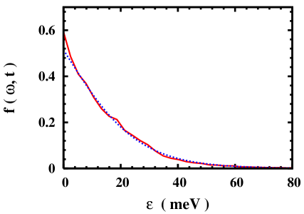
Figure 15: (Color online) The hot-electron distribution in energy space at $t=23$ ps (solid curve) and the fitting curve (dashed curve). $E=1.5$ kV/cm, $T=50$ K, and $N_{i}=0.05N_{e}$.

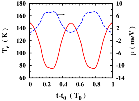
Figure 16: (Color online) The hot-electron temperature $T_{e}$ (solid curves) and the chemical potential $\mu$ (dashed curves) as function of $t$. $E=1.5$ kV/cm, $T=50$ K and $N_{i}=0.05N_{e}$. Note that the scale for the dashed curve is on the right hand side of the frame.

From Fig. 14(b) one further finds that when the SOC is included, the steady-state distributions still have good periodic behavior. The system approaches steady state within 3 ps and the period is again close to $T_{0}$. The distribution difference on the two Floquet states in Fig. 14(a) is due to the spin polarization whereas in Fig. 14(b) is caused by the spectral difference of the two Floquet states.

Appendix C Hot-electron effect and hot-electron temperature

As has been shown in Appendix B that the steady-state distribution $\hat{\tilde{\rho}}^{F}_{{\bf k}}(t)$ is a time dependent function which still exhibits good periodicity in our parameter regime. We can extract the distribution in energy space at any time $t$ via Fourier transformation:

$$\hat{F}(\omega,t)\hat{D}(\omega,t)=\sum_{{\bf k}\eta}\tilde{\rho}^{F(\eta\eta)}_{{\bf k}}(t)\hat{D}_{{\bf k}\eta}(\omega,t).$$ (44)

Here $\hat{D}(\omega,t)=\sum_{{\bf k}\eta}\hat{D}_{{\bf k}\eta}(\omega,t)$ is the generalized density of states ($2\times 2$ matrix) where $t$ is the center-of-mass time:Jauho ; Cheng ; Jiang

$$\hat{D}_{{\bf k}\eta}(\omega,t)=\int_{-\infty}^{\infty}\!\!\frac{d{\tau}}{2\pi}e^{i\omega\tau}\Psi_{{\bf k}\eta}(t+\frac{\tau}{2})\Psi_{{\bf k}\eta}^{\dagger}(t-\frac{\tau}{2}).$$ (45)

It has been found that $\hat{D}_{{\bf k}\eta}(\omega,t)$ and $\hat{D}(\omega,t)$ are periodic functions of $t$ with the same period as that of the THz field $T_{0}=2\pi/\Omega$. Therefore, the distribution $\hat{F}(\omega,t)$ is also a periodic function of $t$ with period $T_{0}$. According to the symmetry analysis, $\hat{D}(\omega,t)=D_{\uparrow\uparrow}(\omega,t)\hat{1}-\mbox{Im}\{D_{\uparrow\downarrow}(\omega,t)\}\hat{\sigma}_{y}$.Cheng As the matrices $\hat{1}$ and $\hat{\sigma}_{y}$ form a group, the distribution $\hat{F}(\omega,t)$ should also be decomposed into two parts: $\hat{F}(\omega,t)=f(\omega,t)\hat{1}+s(\omega,t)\hat{\sigma}_{y}$. Equation (44) then turns into [denoting $\hat{\zeta}(\omega,t)=\sum_{{\bf k}\eta}\tilde{\rho}^{F(\eta\eta)}_{{\bf k}}(t)\hat{D}_{{\bf k}\eta}(\omega,t)$]:

$$f(\omega,{t})D_{\uparrow\uparrow}(\omega,{t})-s(\omega,{t})\mbox{Im}\{D_{\uparrow\downarrow}(\omega,{t})\}$$

$$=\zeta^{\uparrow\uparrow}(\omega,{t}),$$ (46)

$$\mbox{}-s(\omega,{t})D_{\uparrow\uparrow}(\omega,{t})+f(\omega,{t})\mbox{Im}\{D_{\uparrow\downarrow}(\omega,{t})\}$$

$$=\mbox{Im}\{\zeta^{\uparrow\downarrow}(\omega,{t})\}.$$ (47)

The solutions of the above equations are given by

$$f = \frac{\zeta^{\uparrow\uparrow}D_{\uparrow\uparrow}-\mbox{Im}\{\zeta^{\uparrow\downarrow}\}\mbox{Im}\{D_{\uparrow\downarrow}\}}{D_{\uparrow\uparrow}^{2}-\big{[}\mbox{Im}\{D_{\uparrow\downarrow}\}\big{]}^{2}},$$ (48)

$$s = \frac{-\mbox{Im}\{\zeta^{\uparrow\downarrow}\}D_{\uparrow\uparrow}+\zeta^{\uparrow\uparrow}\mbox{Im}\{D_{\uparrow\downarrow}\}}{D_{\uparrow\uparrow}^{2}-\big{[}\mbox{Im}\{D_{\uparrow\downarrow}\}\big{]}^{2}}.$$ (49)

One notices that Eq. (C1) is a natural generalization of the distribution in energy space from thermal equilibrium to the nonequilibrium case. It is straightforward to see that in the zero THz field limit the distribution $\hat{F}(\omega,t)$ recovers the Fermi distribution as $\hat{D}_{{\bf k}\eta}(\omega,{t})=\delta(\omega-\bar{\varepsilon}_{{\bf k}\eta})|\xi_{{\bf k}\eta}\rangle\langle\xi_{{\bf k}\eta}|$ and $\tilde{\rho}^{F(\eta\eta)}_{{\bf k}}(t)=f_{F}(\bar{\varepsilon}_{{\bf k}\eta})$ in the zero-field limit ($f_{F}(x)$ is the Fermi distribution function). Therefore from Eq. (C1), $\hat{F}(\omega,t)=f_{F}(\omega)\hat{1}$.

A typical $f(\omega,t)$ is plotted in Fig. 15. We use the hot-electron temperature $T_{e}$ to measure the hot-electron effect. The hot-electron temperature is determined by fitting the tail of $f(\omega,t)$ with Fermi distribution function. We plot the fitted hot-electron temperature $T_{e}$ and the chemical potential $\mu$ in Fig. 16 ($t_{0}$ in the figure denotes the starting time which is 21.5 ps). It is seen in Fig. 16 that $T_{e}$ and $\mu$ are also periodic functions of $t$ with periodicity of $T_{0}/2$. This is because these quantities only depend on the strength of the THz field. The hot-electron temperature used in Sec. III is the largest temperature, which is sufficient in measuring the hot-electron effect.

References

- (1) Semiconductor Spintronics and Quantum Computation, ed. by D. D. Awschalom, D. Loss, and N. Samarth (Springer-Verlag, Berlin, 2002); I. Žutić, J. Fabian, and S. Das Sarma, Rev. Mod. Phys. 76, 323 (2004); J. Fabian, A. Matos-Abiague, C. Ertler, P. Stano, and I. Žutić, acta physica slovaca 57, 565 (2007); and references therein.
- (2) S. A. Wolf, D. D. Awschalom, R. A. Buhrman, J. M. Daughton, S. von Molnár, M. L. Roukes, A. Y. Chtchelkanova, and D. M. Treger, Science 294, 1488 (2001).
- (3) R. Hanson, L. P. Kouwenhoven, J. R. Petta, S. Tarucha, and L. M. K. Vandersypen, Rev. Mod. Phys. 79, 1217 (2007); and references therein.
- (4) G. Salis, Y. Kato, K. Ensslin, D. C. Driscoll, A. C. Gossard, and D. D. Awschalom, Nature 414, 619 (2001).
- (5) Y. Tokura, W. G. van der Wiel, T. Obata, and S. Tarucha, Phys. Rev. Lett. 96, 047202 (2006).
- (6) E. I. Rashba and Al. L. Efros, Phys. Rev. Lett. 91, 126405 (2003).
- (7) E. I. Rashba and Al. L. Efros, Appl. Phys. Lett. 83, 5295 (2003).
- (8) E. I. Rashba, J. Supercond.: Incorp. Noval Mechanism 18, 137 (2005).
- (9) J. L. Cheng and M. W. Wu, Appl. Phys. Lett. 86, 032107 (2005).
- (10) Al. L. Efros and E. I. Rashba, Phys. Rev. B 73, 165325 (2006).
- (11) M. Duckheim and D. Loss, Nature Phys. 2, 195 (2006); Phys. Rev. B 75, 201305(R) (2007).
- (12) Y. Zhou, Physica E 40, 2847 (2008).
- (13) M. Valín-Rodríguez, A. Puente, and L. Serra, Phys. Rev. B 66, 045317 (2002).
- (14) J. H. Jiang, M. Q. Weng, and M. W. Wu, J. Appl. Phys. 100, 063709 (2006).
- (15) V. N. Golovach, M. Borhani, and D. Loss, Phys. Rev. B 74, 165319 (2007).
- (16) P. Stano and J. Fabian, Phys. Rev. B 77, 045310 (2008).
- (17) D. V. Bulaev and D. Loss, Phys. Rev. Lett. 98, 097202 (2007).
- (18) M. Q. Weng, M. W. Wu, and Q. W. Shi, Phys. Rev. B 69, 125310 (2004); L. Jiang, M. Q. Weng, M. W. Wu, and J. L. Cheng, J. Appl. Phys. 98, 113702 (2005).
- (19) Y. V. Pershin, Phys. Rev. B 75, 165320 (2007).
- (20) Y. A. Bychkov and E. Rashba, Sov. Phys. JETP Lett. 39, 78 (1984).
- (21) G. Dresselhaus, Phys. Rev. 100, 580(1955).
- (22) F. Meier and B. P. Zakharchenya, Optical Orientation (North-Holland, Amsterdam, 1984).
- (23) Y. Kato, R. C. Myers, D. C. Driscoll, A. C. Gossard, J. Levy, D. D. Awschalom, Science 299, 1201 (2003).
- (24) Y. Kato, R. C. Myers, A. C. Gossard, and D. D. Awschalom, Nature 427, 50 (2004).
- (25) S. A. Crooker and D. L. Smith, Phys. Rev. Lett. 94, 236601 (2005).
- (26) L. Meier, G. Salis, I. Shorubalko, E. Gini, S. Schön, and K. Ensslin, Nature Phys. 3, 650 (2007).
- (27) K. C. Nowack, F. H. L. Koppens, Yu. V. Nazarov, and L. M. K. Vandersypen, Science 318, 1430 (2007).
- (28) D. Grundler, Phys. Rev. Lett. 84, 6074 (2000).
- (29) Y. Sato, T. Kita, S. Gozu, and S. Yamada, J. Appl. Phys. 89, 8017 (2001).
- (30) A. P. Jauho and K. Johnsen, Phys. Rev. Lett. 76, 4576 (1996); K. Johnsen and A. P. Jauho, Phys. Rev. B 57, 8860 (1998).
- (31) J. Kono, M. Y. Su, T. Inoshita, T. Noda, M. S. Sherwin, S. J. Allen, Jr., and H. Sakaki, Phys. Rev. Lett. 79, 1758 (1997); A. V. Maslov and D. S. Citrin, Phys. Rev. B 62, 16686 (2000).
- (32) K. B. Nordstrom, K. Johnsen, S. J. Allen, A. P. Jauho, B. Birnir, J. Kono, T. Noda, H. Akiyama, and H. Sakaki, Phys. Rev. Lett. 81, 457 (1998).
- (33) M. Grifoni and P. Hänggi, Phys. Rep. 304, 229 (1998).
- (34) S. Kohler, J. Lehmann, and P. Hänggi, Phys. Rep. 406, 379 (2005).
- (35) For review on intense THz applications to semiconductors and low-dimensional semiconductor structures, see S. D. Ganichev and W. Prettl, Intense Terahertz Excitation of Semiconductors (Oxford University Press, Oxford, 2006).
- (36) J. H. Jiang and M. W. Wu, Phys. Rev. B 75, 035307 (2007).
- (37) For brief review, see M. W. Wu, M. Q. Weng, and J. L. Cheng, in Physics, Chemistry and Application of Nanostructures: Reviews and Short Notes to Nanomeeting 2007, eds. V. E. Borisenko, V. S. Gurin, and S. V. Gaponenko (World Scientific, Singapore, 2007) pp. 14, and references therein.
- (38) M. W. Wu and H. Metiu, Phys. Rev. B 61, 2945 (2000); M. W. Wu and C. Z. Ning, Eur. Phys. J. B 18, 373 (2000); M. W. Wu, J. Phys. Soc. Jpn. 70, 2195 (2001).
- (39) M. Q. Weng and M. W. Wu, Phys. Rev. B 70, 195318 (2004); L. Jiang and M. W. Wu, ibid. 72, 033311 (2005).
- (40) C. Lü, J. L. Cheng, and M. W. Wu, Phys. Rev. B 73, 125314 (2006).
- (41) M. Q. Weng and M. W. Wu, Phys. Rev. B 68, 075312 (2003).
- (42) M. Q. Weng, M. W. Wu, and L. Jiang, Phys. Rev. B 69, 245320 (2004).
- (43) J. L. Cheng and M. W. Wu, J. Appl. Phys. 99, 083704 (2006); ibid. 102, 019901 (2007).
- (44) J. Zhou, J. L. Cheng, and M. W. Wu, Phys. Rev. B 75, 045305 (2007).
- (45) P. Zhang and M. W. Wu, Phys. Rev. B 76, 193312 (2007).
- (46) J. Zhou and M. W. Wu, Phys. Rev. B 77, 075318 (2008).
- (47) D. Stich, J. H. Jiang, T. Korn, R. Schulz, D. Schuh, W. Wegscheider, M. W. Wu, and C. Schüller, Phys. Rev. B 76, 073309 (2007).
- (48) A. W. Holleitner, V. Sih, R. C. Myers, A. C. Gossard, and D. D. Awschalom, New J. Phys. 9, 342 (2007).
- (49) D. Stich, J. Zhou, T. Korn, R. Schulz, D. Schuh, W. Wegscheider, M. W. Wu, and C. Schüller, Phys. Rev. Lett. 98, 176401 (2007); Phys. Rev. B 76, 205301 (2007).
- (50) S. Kohler, T. Dittrich, and P. Hänggi, Phys. Rev. E 55, 300 (1997).
- (51) H. Haug and A. P. Jauho, Quantum Kinetics in Transport and Optics of Semiconductors (Springer, Berlin, 1996).
- (52) J. H. Shirley, Phys. Rev. 138, B979 (1965).
- (53) C. W. Gardiner and P. Zoller, Quantum Noise (Springer, Berlin, 2000).
- (54) See, for example, Magneto-Optics, edt. by S. Sugano and N. Kojima (Springer-Verlag, Berlin, 1999).
- (55) J. J. Baumberg, D. D. Awschalom, and N. Samarth, J. Appl. Phys. 75, 6199 (1994).
- (56) G. Ramian, Nucl. Instrum. Methods Phys. Res. Sect. A 318, 225 (1992).
- (57) Semiconductors, Landolt-Börnstein, New Series, Vol. 17a, ed. by O. Madelung (Springer-Verlag, Berlin, 1987).
- (58) V. V. Bel’kov, S. D. Ganichev, E. L. Ivchenko, S. A. Tarasenko, W. Weber, S. Giglberger, M. Olteanu, H.-P. Tranitz, S. N. Danilov, P. Schneider, W. Wegscheider, D. Weiss, and W Prettl, J. Phys.: Condens. Matter 17, 3405 (2005).
- (59) S. D. Ganichev, S. N. Danilov, P. Schneider, V. V. Bel’kov, L. E. Golub, W. Wegscheider, D. Weiss, and W. Prettl, J. Magn. Magn. Mater. 300, 127 (2006).
- (60) V. V. Bel’kov and S. D. Ganichev, arXiv:0803.0949.
- (61) W. J. H. Leyland, R. T. Harley, M. Henini, A. J. Shields, I. Farrer, and D. A. Ritchie, Phys. Rev. B 76, 195305 (2007).
- (62) X. L. Lei and C. S. Ting, Phys. Rev. B 30, 4809 (1984).
- (63) X. L. Lei, J. Appl. Phys. 84, 1396 (1998); J. Phys.: Condens. Matter 10, 3201 (1998).
- (64) M. M. Glazov and E. L. Ivchenko, Zh. Éksp. Teor. Fiz. 126, 1465 (2004) [JETP 99, 1279 (2004)]; Pis’ma Zh. Éksp. Teor. Fiz. 75, 476 (2002) [JETP Lett. 75, 403 (2002)].
- (65) X. Z. Ruan, H. H. Luo, Y. Ji, Z. Y. Xu, and V. Umansky, Phys. Rev. B 77, 193307 (2008).