Collective neutrino oscillations in non-spherical geometry

Abstract

The rich phenomenology of collective neutrino oscillations has been studied only in one-dimensional or spherically symmetric systems. Motivated by the non-spherical example of coalescing neutron stars, presumably the central engines of short gamma-ray bursts, we use the Liouville equation to formulate the problem for general source geometries. Assuming the neutrino ensemble displays self-maintained coherence, the problem once more becomes effectively one-dimensional along the streamlines of the overall neutrino flux. This approach for the first time provides a formal definition of the “single-angle approximation” frequently used for supernova neutrinos and allows for a natural generalization to non-spherical geometries. We study the explicit example of a disk-shaped source as a proxy for coalescing neutron stars.

I Introduction

Flavor transformations caused by neutrino mixing depend on the matter background and on the neutrino fluxes themselves: neutrino-neutrino interactions provide a nonlinear term in the equations of motion Pantaleone:1992eq ; Sigl:1992fn that gives rise to collective flavor transformation phenomena Samuel:1993uw ; Kostelecky:1993dm ; Kostelecky:1995dt ; Samuel:1996ri ; Pastor:2001iu ; Wong:2002fa ; Abazajian:2002qx ; Pastor:2002we ; Sawyer:2004ai ; Sawyer:2005jk ; Sawyer:2008zs . The neutrino density needs to be so large that a typical neutrino-neutrino interaction energy $\mu$ is comparable to the vacuum oscillation frequency $\omega=\Delta m^{2}/2E$. Only recently has it been fully appreciated that this condition is sufficient even if a dense background of ordinary matter provides a much larger interaction energy so that naively neutrino-neutrino interactions would seem negligible Duan:2005cp ; Duan:2006an . Following this crucial insight, nonlinear oscillation phenomena in the supernova (SN) context have been studied over the past two years in a long series of papers Duan:2006an ; Hannestad:2006nj ; Duan:2007mv ; Raffelt:2007yz ; EstebanPretel:2007ec ; Raffelt:2007cb ; Raffelt:2007xt ; Duan:2007fw ; Fogli:2007bk ; Duan:2007bt ; Duan:2007sh ; Dasgupta:2008cd ; EstebanPretel:2007yq ; Dasgupta07 ; Duan:2008za ; Dasgupta:2008my ; Duan:2008eb .

One striking effect is “self-maintained coherence” Samuel:1993uw ; Kostelecky:1993dm ; Kostelecky:1995dt ; Samuel:1996ri . Different neutrino modes have different vacuum oscillation frequencies $\omega=\Delta m^{2}/2E$, but with strong neutrino-neutrino interactions they “stick together” and oscillate as a single mode characterized by the “synchronized oscillation frequency” $\omega_{\rm sync}=\langle\Delta m^{2}/2E\rangle$. This can lead to all modes going through an MSW resonance together, the “collective MSW-like transition” or “synchronized MSW effect” Wong:2002fa ; Abazajian:2002qx ; Duan:2007fw ; Duan:2007sh ; Dasgupta:2008cd .

More interesting still are collective phenomena driven by the decrease of the neutrino flux with distance from the source. The adiabatic transition from a dense to a dilute neutrino gas produces step-like spectral features where the spectrum sharply splits into parts of different flavor transformation, so-called “step-wise spectral swapping” or “spectral splits” Duan:2006an ; Raffelt:2007cb ; Raffelt:2007xt ; Duan:2007fw ; Duan:2007bt ; Fogli:2007bk ; Duan:2007sh ; Dasgupta:2008cd ; Duan:2008za . Spectral splits can result from a preceding collective MSW effect (“MSW prepared spectral split”) or from neutrino-neutrino interactions alone.

The latter case depends on an unusual form of non-equilibrium among neutrino flavors where one has an excess of flavor pairs, say $\nu_{e}\bar{\nu}_{e}$, over the other flavors. For neutrinos streaming off a SN core one indeed expects a hierarchy of number fluxes $F_{\nu_{e}}>F_{\bar{\nu}_{e}}>F_{\nu_{\mu},\nu_{\tau}}=F_{\bar{\nu}_{\mu},\bar{\nu}_{\tau}}$. Therefore, one can have collective transformations of the form $\nu_{e}\bar{\nu}_{e}\to\nu_{x}\bar{\nu}_{x}$, where $x$ stands for some suitable combination of $\mu$ and $\tau$ neutrinos. These “collective pair transformations” do not violate any conservation law and thus can be catalyzed even by a very small mixing angle. $F_{\bar{\nu}_{e}}$ can completely swap with $F_{\bar{\nu}_{x}}$ whereas the larger $F_{\nu_{e}}$ converts only to the extent allowed by flavor-lepton conservation, but in a step-like spectral form. Both the complete conversion of $F_{\bar{\nu}_{e}}$ and the split in the $\nu_{e}$ spectrum provide signatures for the inverted neutrino hierarchy even for an extremely small 13-mixing angle Duan:2007bt ; Dasgupta:2008my .

For non-isotropic enviroments, multi-angle effects may play an important role. The term “multi-angle effects” actually refers to two different issues. One is that the weak interaction potential between two relativistic particles is proportional to ($1-\cos\theta$), where $\theta$ is their relative angle of propagation. One usually considers an isotropic background of ordinary matter so that $\cos\theta$ averages to zero. The same is true in an isotropic neutrino gas for the neutrino-neutrino term. The second issue is the “multi-angle instability”. Neutrinos arriving from different points on the source belong to different angular modes, which may decohere kinematically in flavor space Sawyer:2004ai ; Sawyer:2005jk ; Sawyer:2008zs ; Raffelt:2007yz ; EstebanPretel:2007ec . This effect can be self-induced in the sense that a very small initial anisotropy is enough to trigger an exponential runaway, for example in a gas consisting of equal densities of neutrinos and antineutrinos Raffelt:2007yz . Systems consisting of very few angular modes can show a two-stream or multi-stream instability Sawyer:2004ai ; Sawyer:2005jk ; Sawyer:2008zs . On the other hand, numerical studies show that systems consisting of many angular modes and with a sufficient neutrino-antineutrino asymmetry do not show a multi-angle instability but rather show self-maintained coherence among different angular modes Duan:2006an ; EstebanPretel:2007ec ; Fogli:2007bk . The SN neutrino flux parameters seem to be such that the multi-angle instability plays no role in practice. Based on this assumption, most of the SN studies have used the “single-angle approximation”, where all angular modes are assumed to have the same behavior.

Multi-angle effects related to the ($1-\cos\theta$) structure of the neutrino-neutrino term are unavoidable for an extended source radiating neutrinos into space because the emitted neutrino flux cannot form an isotropic gas. However, these effects also occur, and are easier to study theoretically, in a homogeneous system evolving in time that has a non-isotropic angular distribution of neutrinos.

In practice, however, one usually deals with stationary systems where one asks for the spatial variation of a neutrino ensemble as a function of distance from the source. Even if the neutrino-neutrino interaction were isotropic, we still would have geometric multi-angle effects because neutrinos reaching a certain point from an extended source have traveled on different trajectories. Even the simple case of an infinite radiating plane is not trivial. Here the direction perpendicular to the plane is the only direction in which the overall neutrino ensemble can show any spatial variation. Even if all neutrinos have the same energy and thus oscillate with the same frequency along their trajectories, the projection on the direction perpendicular to the plane yields different effective oscillation frequencies and thus kinematical decoherence. Neutrino-neutrino effects can synchronize different angular modes so that a sufficiently dense neutrino gas will not show this form of multi-angle decoherence. On the contrary, all angular modes will vary with the same oscillation length as a function of distance from the plane. A similar description applies to a spherical source where one asks for the variation of all angular modes along the radial direction.

The single-angle treatment of SN neutrino oscillations amounts to the assumption of self-maintained coherence among angular modes, although it has never been explicitly expressed in this form. Some authors assumed that all angular modes oscillate as the radial one Duan:2006an . However, in this case the neutrino-neutrino interaction vanishes because of the ($1-\cos\theta$) factor, so it was necessary to assume a certain average of the neutrino-neutrino interaction strength. Other authors represented all angular modes by a single angular mode radiated at $45^{\circ}$ relative to the radial direction and then used a neutrino-neutrino interaction strength consistent with this assumption EstebanPretel:2007yq . This implementation of the single-angle approximation has the advantage that one can use the same numerical code as for multi-angle simulations, simply restricting oneself to a single angular bin. In yet other cases the system was modeled as a homogeneous and isotropic gas that evolves in time, assuming a time variation of the neutrino density that mimics the radial variation in the spherical case.

One of our goals is to show that the single-angle treatment can be formulated self-consistently. The assumption that all angular modes evolve the same in flavor space provides a unique concept of what is meant by “single-angle behavior.” This is straightforward in the systems described so far where symmetry dictates that the spatial variation is only along a certain direction, effectively reducing the problem to one dimension. We are really motivated, however, by more general geometries where no special direction is singled out by symmetry. In particular, we are interested in the case of coalescing neutron stars that may form the inner engines of short gamma-ray bursts Ruffert:1998qg .

The accretion torus or disk formed during neutron star coalescence is a neutrino source comparable to a SN core. However, the torus is less dense and not efficient at producing $\nu_{\mu}$ and $\nu_{\tau}$. Therefore, the torus is a source for a dominant $\nu_{e}\bar{\nu}_{e}$ pair flux which is thought to produce an $e^{+}e^{-}$ pair plasma, thus powering short gamma-ray bursts. The annihilation cross section for $\nu_{e}\bar{\nu}_{e}\to e^{+}e^{-}$ is much larger than that for $\nu_{x}\bar{\nu}_{x}\to e^{+}e^{-}$, so the neutrino flavor composition strongly influences the number of $e^{+}e^{-}$ pairs produced. Therefore, one may ask if collective pair conversions occur in this environment close enough to the source to modify the energy transfer to the $e^{+}e^{-}$ plasma, and hence affect the strength of the gamma ray burst.

For coalescing neutron stars one expects a flux hierarchy $F_{\bar{\nu}_{e}}>F_{\nu_{e}}\gg F_{\nu_{x}}=F_{\bar{\nu}_{x}}$, which differs from the SN case because the matter leptonizes when neutrons convert to protons, in contrast to the deleptonization of a SN core. The asymmetry between $F_{\nu_{e}}$ and $F_{\bar{\nu}_{e}}$ could be enough to prevent multi-angle decoherence so that similar collective effects as in the SN environment are conceivable. However, even granting this assumption, it is not straightforward how to implement something like a single-angle approximation in this context because it is not obvious how one should picture self-maintained coherence.

The purpose of our paper is to formulate the meaning of self-maintained coherence for general source geometries and study its implications. We find that the flavor variation reduces to a quasi one-dimensional problem along the streamlines of the total neutrino flux. The main difference between the general case and the radiating plane or sphere is that the streamlines are typically curved, at least close to the source, so that self-maintained coherence applies to flavor oscillations along these curved streamlines.

We begin in Sec. II with the general equations of motion for the neutrino matrices in flavor space. In Sec. II.2 we formulate the collective equations for neutrinos only (no antineutrinos) and consider only synchronized oscillations. Sec. II.3 shows the existence of streamlines and gives a prescription for calculating the flavor evolution along them. In Sec. III we solve the problem for several geometries. In Sec. IV we study the generalization to a mixed system of neutrinos and antineutrinos where collective pair transformations are possible. In Sec. V we consider an explicit example for a disk source with parameters inspired by numerical simulations of coalescing neutron stars. We summarize our conclusions in Sec. VI.

II Formalism for an arbitrary source geometry

II.1 General framework

A homogeneous ensemble of mixed neutrinos can be described by “matrices of density” $\varrho_{\bf p}$, which really are matrices of occupation numbers, for each momentum mode ${\bf p}$ Dolgov:1980cq ; Rudzsky:1990 ; Sigl:1992fn ; mckellar&thomson . If $a^{\dagger}_{i,{\bf p}}$ and $a_{i,{\bf p}}$ are the creation and annihilation operators of a neutrino in the mass eigenstate $i$ of momentum ${\bf p}$, we have $(\varrho_{\bf p})_{ij}\propto\langle a^{\dagger}_{j}a_{i}\rangle_{\bf p}$ so that the diagonal entries of $\varrho_{\bf p}$ are the usual occupation numbers (expectation values of number operators), whereas the off-diagonal elements encode the phase relations that allow one to follow flavor oscillations. Such a description assumes that higher-order correlations beyond field bilinears play no role, probably a good approximation for neutrinos produced from essentially thermal sources such as the early-universe plasma or a SN core.

Antineutrinos are described in an analogous way by $(\bar{\varrho}_{\bf p})_{ij}=\langle\bar{a}^{\dagger}_{i}\bar{a}_{j}\rangle_{\bf p}$. Note that we always use overbars to characterize antiparticle quantities. The order of flavor indices was deliberately interchanged on the r.h.s. so that the matrices $\varrho_{\bf p}$ and $\bar{\varrho}_{\bf p}$ transform in the same way in flavor space Sigl:1992fn . In this way one can, for example, write the overall neutrino current in the simple form $\int{\rm d}{\bf p}\,v_{\bf p}(\varrho_{\bf p}-\bar{\varrho}_{\bf p})$ where here and henceforth ${\rm d}{\bf p}$ stands for ${\rm d}^{3}{\bf p}/(2\pi)^{3}$. While some authors prefer the seemingly more intuitive equal order of flavor indices for neutrinos and antineutrinos, in that convention the current would be $\int{\rm d}{\bf p}\,v_{\bf p}(\varrho_{\bf p}-\bar{\varrho}_{\bf p}^{*})$ and generally the equations will involve both the matrices of density and their complex conjugates. (In a truly field-theoretic derivation there is no ambiguity about the relative structure of neutrino and antineutrino matrices. An analogous example for matrices of occupation numbers is provided by the kinetic treatment of the quark–gluon plasma where the quark distribution functions are $3\times 3$ matrices in color space Mrowczynski:2007hb . The matrices for quarks and the ones for antiquarks transform equally under a color gauge transformation.)

The matrices $\varrho_{\bf p}$ and $\bar{\varrho}_{\bf p}$ depend on time. Their evolution is governed by the Boltzmann collision equation

$$\partial_{t}\varrho_{\bf p}=-{\rm i}[{\sf\Omega}_{\bf p},\varrho_{\bf p}]+\dot{\varrho}_{\bf p}\big{|}_{\rm coll}$$ (1)

and a similar equation for $\bar{\varrho}_{\bf p}$. The collision term will be of no further concern in our paper because we only study freely streaming neutrinos. Further, $[\cdot,\cdot]$ is a commutator and ${\sf\Omega}_{\bf p}$ is the matrix of oscillation frequencies. In vacuum we have ${\sf\Omega}_{\rm p}={\sf M}^{2}/2|{\bf p}|$ with ${\sf M}$ the neutrino mass matrix. In general ${\sf\Omega}_{\rm p}$ also depends on the background medium and notably on the presence of other neutrinos. Here and henceforth the ultrarelativistic limit for neutrinos is assumed. In other words, it is assumed that the difference between the neutrino energy $E_{\bf p}$ and momentum $p=|{\bf p}|$ is irrelevant except for oscillations: the only relevant difference between energy and momentum is captured by the matrix of oscillation frequencies.

Up to this point we have considered a homogeneous ensemble evolving in time, largely relevant for neutrino oscillations in the early universe for which this formalism was originally developed. However, for a realistic representation of radiating objects such as supernovae or coalescing neutron stars we need to include spatial transport phenomena. To this end one introduces space-dependent occupation numbers or Wigner functions $\varrho_{\bf p,x}$. The quantum-mechanical uncertainty between location and momentum implies that this construction is only valid in the limit where spatial variations of the ensemble are weak on the microscopic length scales defined by the particles’ typical Compton wavelengths. The left hand side of the Boltzmann collision equation now turns into the usual Liouville operator Strack:2005ux

$$\partial_{t}\varrho_{\bf p,x}+{\bf v}_{\bf p}\cdot{\nabla}_{\bf x}\,\varrho_{\bf p,x}+\dot{\bf p}\cdot{\nabla}_{\bf p}\,\varrho_{\bf p,x}.$$ (2)

The transition to the Liouville operator may seem obvious, but making it conceptually precise requires a long argument Cardall:2007zw . The first term represents an explicit time dependence, the second a drift term caused by the particles’ free streaming, and the third the effect of external macroscopic forces, for example gravitational deflection. Henceforth we shall neglect external forces and only retain the drift term.

In our ultrarelativistic approximation the modulus of ${\bf v}_{\bf p}$ is the speed of light. Of course, for propagation over very large distances this may be a bad approximation when time-of-flight effects play a role. In this case the drift term would have a more complicated structure because the velocity is then also a nontrivial matrix in flavor space Sigl:1992fn .

We shall focus on stationary problems. Even neutrino emission from a SN or coalescing neutron stars fall in this category unless there are fast variations of the source. In other words, we shall ignore a possible explicit time dependence of $\varrho_{\bf p,x}$ so that finally we arrive at

$${\bf v}_{\bf p}\cdot{\bf\nabla}_{\bf x}\,\varrho_{\bf p,x}=-{\rm i}[{\sf\Omega}_{\bf p,x},\varrho_{\bf p,x}]\,,$$ (3)

where the matrix of oscillation frequencies in general also depends on space because of the influence of matter and other neutrinos.

Equation (3) could have been guessed starting from the usual treatment of neutrino oscillations. The neutrino density matrix describing a stationary beam in the $z$–direction follows $\partial_{z}\varrho_{E,z}=-{\rm i}[\Omega_{E,z},\varrho_{E,z}]$. Moreover, in our ultrarelativistic approximation $E=p$ and $|{\bf v}_{\bf p}|=1$. Equation (3) then simply amounts to a collection of many beams in different directions originating from different source points.

We finally spell out Eq. (3) explicitly under the assumption that the only nontrivial ingredients consist of neutrino-neutrino refractive effects,

$${\rm i}\,{\bf v}_{\bf p}\cdot{\bf\nabla}_{\bf x}\,\varrho_{\bf p,x} = +\frac{1}{2p}\,\bigl{[}{\sf M}^{2},\varrho_{\bf p,x}\bigr{]}+\sqrt{2}\,G_{\rm F}\int{\rm d}{\bf q}\,(1-{\bf v}_{\bf q}\cdot{\bf v}_{\bf p})\bigl{[}(\varrho_{\bf q,x}-\bar{\varrho}_{\bf q,x}),\varrho_{\bf p,x}\bigr{]}\,,$$

$${\rm i}\,{\bf v}_{\bf p}\cdot{\bf\nabla}_{\bf x}\,\bar{\varrho}_{\bf p,x} = -\frac{1}{2p}\,\bigl{[}{\sf M}^{2},\bar{\varrho}_{\bf p,x}\bigr{]}+\sqrt{2}\,G_{\rm F}\int{\rm d}{\bf q}\,(1-{\bf v}_{\bf q}\cdot{\bf v}_{\bf p})\bigl{[}(\varrho_{\bf q,x}-\bar{\varrho}_{\bf q,x}),\bar{\varrho}_{\bf p,x}\bigr{]}\,.$$ (4)

The only difference between the neutrino and antineutrino equations is the sign of the vacuum oscillation term. This structure is a consequence of defining the antineutrino matrices with reversed flavor indices.

II.2 EOMs with self-maintained coherence

The nonlinear equations of motion (EOMs) Eq. (II.1) simplify considerably if self-maintained coherence occurs in a dense neutrino gas and all modes can be assumed to evolve in the same way. For the moment we restrict ourselves to a source radiating only neutrinos (no antineutrinos). What we mean by self-maintained coherence in this case is that at a given location all neutrino modes are aligned with each other, assuming they were aligned at the source. That is,

$$\varrho_{\bf p,x}={\sf P}_{\bf x}\,f_{\bf p,x}\,.$$ (5)

Here, $f_{\bf p,x}={\rm Tr}(\varrho_{\bf p,x})$ is a scalar occupation number, summed over all flavors, while for $N$ flavors ${\sf P}_{\bf x}$ is a $N\times N$ matrix normalized as ${\rm Tr}({\sf P}_{\bf x})=1$. We also define the local neutrino density and flux as

$$n_{\bf x} = \int{\rm d}{\bf p}\,f_{\bf p,x}\,,$$

$${\bf F}_{\bf x} = \int{\rm d}{\bf p}\,{\bf v}_{\bf p}\,f_{\bf p,x}\,=\langle{\bf v}\rangle_{\bf x}n_{\bf x}\;,$$ (6)

where

$$\langle Q\rangle_{\bf x}\equiv\frac{\int{\rm d}{\bf p}\,Q_{\bf p,x}\,f_{\bf p,x}}{\int{\rm d}{\bf p}\,f_{\bf p,x}}$$ (7)

is the momentum average of a quantity $Q$ at location ${\bf x}$ with respect to the distribution function $f_{\bf p,x}$. For future convenience we also define

$$\widehat{\bf F}_{\bf x}\equiv\frac{{\bf F}_{\bf x}}{|{\bf F}_{\bf x}|}=\frac{\langle{\bf v}\rangle_{\bf x}}{|\langle{\bf v}\rangle_{\bf x}|}\;,$$ (8)

a unit vector along the direction of flux ${\bf F}_{\bf x}$, or equivalently, along the average velocity $\langle{\bf v}\rangle_{\bf x}$.

In this language, the EOM Eq. (II.1) becomes

$${\bf v}_{\bf p}\cdot{\bf\nabla}_{\bf x}\,f_{\bf p,x}{\sf P}_{\bf x}=-\frac{{\rm i}}{2p}\,\bigl{[}{\sf M}^{2},{\sf P}_{\bf x}\bigr{]}\,f_{\bf p,x}\,,$$ (9)

where the nonlinear term has disappeared because it involves the commutator $[{\sf P}_{\bf x},{\sf P}_{\bf x}]=0$. The only impact of the neutrino-neutrino term is to glue the different modes together, but afterwards it no longer appears in the equation.

The evolution now factorizes into the free streaming of the overall neutrino flux and the oscillation of the common flavor matrix ${\sf P}_{\bf x}$. The trace of Eq. (9) provides

$${\bf v}_{\bf p}\cdot{\bf\nabla}_{\bf x}\,f_{\bf p,x}=0\,,$$ (10)

allowing us to determine the overall neutrino density $n_{\bf x}$ and flux ${\bf F}_{\bf x}$ at any point, assuming it is given at the source surface. With ${\bf v}_{\bf p}\cdot{\bf\nabla}_{\bf x}\,f_{\bf p,x}={\bf\nabla}_{\bf x}\cdot{\bf v}_{\bf p}\,f_{\bf p,x}$, integrating Eq. (10) over all modes yields

$${\bf\nabla}_{\bf x}\cdot{\bf F}_{\bf x}=0\,,$$ (11)

expressing the absence of neutrino sources or sinks.

The EOM for ${\sf P}_{\bf x}$ is found by integrating Eq. (9) over all modes,

$${\bf\nabla}_{\bf x}\cdot\bigl{(}{\bf F}_{\bf x}\,{\sf P}_{\bf x}\bigr{)}=-\frac{{\rm i}}{2}\,\bigl{[}{\sf M}^{2},{\sf P}_{\bf x}\bigr{]}\,\int{\rm d}{\bf p}\,\frac{f_{\bf p,x}}{p}\,.$$ (12)

The l.h.s. expands as $\bigl{(}{\bf\nabla}_{\bf x}\cdot{\bf F}_{\bf x}\bigr{)}\,{\sf P}_{\bf x}+{\bf F}_{\bf x}\cdot\bigl{(}{\bf\nabla}_{\bf x}{\sf P}_{\bf x}\bigr{)}$ where the first term disappears because of Eq. (11) so that

$${\bf F}_{\bf x}\cdot{\bf\nabla}_{\bf x}{\sf P}_{\bf x}=-\frac{{\rm i}}{2}\,\bigl{[}{\sf M}^{2},{\sf P}_{\bf x}\bigr{]}\,\int{\rm d}{\bf p}\,\frac{f_{\bf p,x}}{p}\,.$$ (13)

Dividing both sides by $|{\bf F}_{\bf x}|$, we get

$$\widehat{\bf F}_{\bf x}\cdot{\bf\nabla}_{\bf x}{\sf P}_{\bf x}=-{\rm i}\,\bigl{[}{\sf\Omega}_{\bf x},{\sf P}_{\bf x}\bigr{]}\,,$$ (14)

where

$${\sf\Omega}_{\bf x}=\frac{{\sf M}^{2}}{2}\,\frac{\int{\rm d}{\bf p}\,p^{-1}\,f_{\bf p,x}}{\left|\int{\rm d}{\bf p}\,{\bf v}_{\bf p}\,f_{\bf p,x}\right|}=\frac{{\sf M}^{2}}{2}\,\frac{\langle p^{-1}\rangle}{|\langle{\bf v}\rangle_{\bf x}|}\,.$$ (15)

Equation (14) resembles the EOM in the single-angle approximation, with $\Omega_{\bf x}$ as the synchronized matrix of oscillation frequencies. Note that $\langle p^{-1}\rangle$ is independent of location if the energy spectrum of neutrinos is assumed to be the same everywhere.

II.3 Streamlines

Equation (14) is a partial differential equation (PDE) for the matrix ${\sf P}_{\bf x}$. It can be reduced to a set of ordinary differential equations (ODEs)

$$\frac{{\rm d}{\bf x}}{{\rm d}s} = \widehat{\bf F}_{\bf x}\;,$$ (16)

$$\frac{{\rm d}{\sf P}_{\bf x}}{{\rm d}s} = -{\rm i}\,\bigl{[}{\sf\Omega}_{\bf x},{\sf P}_{\bf x}\bigr{]}\,,$$ (17)

where $s$ is a parameter along the “characteristic line,” or “streamline,” defined by Eq. (16). Since $\widehat{\bf F}_{\bf x}$ is unique at each location, the streamlines do not intersect each other. Along each streamline, the differential equation [Eq. (17)] for the matrix ${\sf P}_{\bf x}$ is a set of coupled, but linear ODEs and hence can be solved easily and uniquely, given the boundary conditions.

As an illustration, we now specialize to a two-flavor system, where the coupled ODEs in Eq. (17) reduce to a single ODE and may be interpreted as the evolution of a single phase. As uaual, we express a Hermitian $2\times 2$ matrix ${\sf A}$ in terms of a polarization vector $\vec{\rm A}$ by virtue of ${\sf A}=\frac{1}{2}({\rm Tr}\,{\sf A}+\vec{A}\cdot\vec{\sigma})$ with $\vec{\sigma}$ the vector of Pauli matrices. The equation for synchronized oscillations then turns into the usual precession formula

$$\widehat{\bf F}_{\bf x}\cdot{\bf\nabla}_{\bf x}\vec{P}_{\bf x}=\omega_{\bf x}\,\vec{B}\times\vec{P}_{\bf x}\,,$$ (18)

where $\vec{P}_{\bf x}$ is the polarization vector corresponding to $\varrho_{\bf x}$ and $\omega_{\bf x}\vec{B}$ the one corresponding to $\sf\Omega_{\bf x}$. Here $\vec{B}$ is a unit vector by definition, which is determined by ${\sf M}^{2}$ and hence is independent of location. The effective synchronized oscillation frequency is

$$\omega_{\bf x}=\frac{\Delta m^{2}}{2}\frac{\langle p^{-1}\rangle}{|\langle{\bf v}\rangle_{\bf x}|}=\frac{\omega_{0}}{|\langle{\bf v}\rangle_{\bf x}|}\;,$$ (19)

where $\omega_{0}$ is the synchronized oscillation frequency far away from the source, where the details of the source geometry do not matter. All the effects of the source geometry are thus captured by the quantity $|\langle{\bf v}\rangle_{\bf x}|$.

The problem becomes even simpler if we observe that the magnitude of $\vec{P}_{\bf x}$ and its projection on $\vec{B}$ are conserved. We can then write $\vec{P}_{\bf x}$ in terms of its components along and perpendicular to $\vec{B}$ as

$$\vec{P}_{\bf x}=(P_{\perp}\cos a_{\bf x},P_{\perp}\sin a_{\bf x},P_{\parallel})\;.$$ (20)

Equation (18) then reduces to a scalar equation

$$\widehat{\bf F}_{\bf x}\cdot{\bf\nabla}_{\bf x}\,a_{\bf x}=\omega_{\bf x}\;.$$ (21)

In other words, $\vec{P}_{\bf x}$ is fully specified by a real scalar number $a_{\bf x}$ that tells us the phase of the revolution of the polarization vector around $\vec{B}$. Equations (16) and (17) in this case simplify to

$$\frac{{\rm d}{\bf x}}{{\rm d}s} = \widehat{\bf F}_{\bf x}=\frac{\langle{\bf v}\rangle_{\bf x}}{|\langle{\bf v}\rangle_{\bf x}|}\;,$$ (22)

$$\frac{{\rm d}a_{\bf x}}{{\rm d}s} = \omega_{\bf x}=\frac{\omega_{0}}{|\langle{\bf v}\rangle_{\bf x}|}\;.$$ (23)

As before, the streamlines are given by Eq. (22) and the evolution is obtained by solving the single ODE in Eq. (23). This has been possible because of a simple parametrization of $\vec{P}_{\bf x}$ in Eq. (20) in two flavors.

In the case of three flavors, one can express a Hermitian $3\times 3$ matrix in terms of the Gell-Mann matrices Dasgupta07 . Equation (18) then retains the same form, except that the “cross product” is now understood to be $(\vec{A}\times\vec{B})_{i}\equiv f_{ijk}A_{j}B_{k}$ with $f_{ijk}$ the structure constants for SU(3). The ODEs in Eq. (17) are coupled, but linear, and can be solved along the streamlines.

The general strategy for calculating the neutrino flavor evolution is therefore the following. $(i)$ Find the streamlines for the problem by solving Eq. (16) with the given neutrino source. $(ii)$ Solve for the phase $a_{\bf x}$ (or for the matrix ${\sf P}_{\bf x}$) by solving the ODEs [Eq. (17)] along each streamline. This leads to the determination of $\varrho_{\bf p,x}$ everywhere.

An important consequence of the existence of streamlines is that the evolution along any streamline is independent of the other streamlines. Moreover, each streamline is determined solely by the flux ${\bf F}_{\bf x}$ along it. Thus the neutrino flavor content at any point in space is determined simply by identifying the streamline that passes through that point and evolving the phase $a_{\bf x}$ along the streamline. This effectively reduces any multi-dimensional problem to one dimension.

III Flavor evolutions for various source geometries

We now calculate the flavor evolution of neutrinos in several physical situations, ranging from the trivial to the complicated. The crucial quantity to calculate in each scenario is $\langle{\bf v}\rangle_{\bf x}$, which captures the effect of the source geometry through Eq. (19).

III.1 Infinite Plane

For a homogeneous plane that radiates neutrinos isotropically, the streamlines are straight lines normal to the surface. Therefore, the oscillation phase $a$ depends only on the distance $z$ from the plane and the surfaces of equal phase are planes parallel to the radiating surface. The average velocity of all neutrinos away from the plane is half the speed of light, $\langle{\bf v}\rangle_{\bf x}=\frac{1}{2}\hat{z}$ everywhere. Therefore, $\omega_{\bf x}=2\omega_{0}$ represents the flavor oscillations along the direction perpendicular to the plane. This gives $a=2\omega_{0}\,z+a_{0}$, where $a_{0}$ may be chosen to be an arbitrary real number. This, along with the initial conditions, completely determines the flavor state of the neutrinos at any point in space.

III.2 Sphere

For a spherical source, symmetry dictates that the streamlines are straight lines following the radial distance from the center and that the surfaces of equal phase are spherical shells around the source. Therefore spherical symmetry dictates that the average velocity $\langle{\bf v}\rangle_{\bf x}=\langle v_{r}\rangle\hat{r}$ is along the radius. All that remains to be determined is $\langle v_{r}\rangle$, the average radial velocity of all neutrinos at distance $r$.

Figure 1: Synchronization frequency $\omega_{r}$ for an emitting sphere (radius $R$) as a function of distance $r$.

To this end we note that all modes that are radiated at the neutrino sphere with the same zenith angle $\vartheta_{R}$ relative to the radial direction behave identically. Their radial velocity at the neutrino sphere is $v_{R}=\cos\vartheta_{R}$, so it is useful to classify all modes by their $v_{R}$. Simple geometry tells us that $R\,\sin\vartheta_{R}=r\sin\vartheta_{r}$, where $\vartheta_{r}$ is the zenith angle of a given neutrino trajectory relative to the radial direction at a distance $r$. Therefore, the radial velocity at distance $r$ of a mode that has radial velocity $v_{R}$ at the neutrino sphere is

$$v_{r}=\cos\vartheta_{r}=\sqrt{1-\frac{R^{2}}{r^{2}}\,\left(1-v_{R}^{2}\right)}\;.$$ (24)

Given the all-flavor phase-space density $f(v_{R},R)$ of a mode $v_{R}$ at the neutrino sphere, we can determine its value $f(v_{R},r)$ at another distance from flux conservation. In spherical coordinates we have $\partial_{r}[r^{2}v_{r}f(v_{R},r)]=0$ so that $f(v_{R},r)\propto(R/r)^{2}(v_{R}/v_{r})$.

If we assume isotropic emission at the neutrino sphere, the modes are uniformly distributed in the variable $0\leq\cos\vartheta_{R}\leq 1$ or $0\leq v_{R}\leq 1$, so that

$$\langle v_{r}\rangle=\frac{\int_{0}^{1}{\rm d}v_{R}\,v_{r}\,f(v_{R},r)}{\int_{0}^{1}{\rm d}v_{R}\,f(v_{R},r)}=\frac{\int_{0}^{1}{\rm d}v_{R}\,v_{R}}{\int_{0}^{1}{\rm d}v_{R}\,v_{R}/v_{r}}\,.$$ (25)

Inserting the expression Eq. (24) for $v_{r}$ and performing the integral we find

$$\langle v_{r}\rangle=\frac{1}{2}\left[1+\sqrt{1-\left(\frac{R}{r}\right)^{2}}\,\right]\,.$$ (26)

At the neutrino sphere ($r=R$) one finds $\langle v_{R}\rangle=\frac{1}{2}$, identical to the radiating plane, whereas at large distances $r\gg R$ all modes move essentially in the radial direction and $\langle v_{r}\rangle\to 1$. Therefore, near the neutrino sphere, the neutrino flavor evolves along the radial direction with frequency $\omega_{r}=2\omega_{0}$, whereas at large distances it evolves with $\omega_{r}=\omega_{0}$. This case is represented in Fig. 1. The decrease of $\omega_{r}$ to its asymptotic value is surprisingly fast. As usual, the phase is given by $a=\int\omega_{r}dr+a_{0}$, and this along with initial conditions specifies the flavour content of neutrinos all over space.

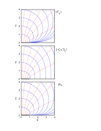
Figure 2: Streamlines for the disk source, combined with contours for various quantities: (a) Neutrino flux $|{\bf F}_{\bf x}|$. (b) Average velocity $|\langle{\bf v}\rangle_{\bf x}|$. (c) Effective neutrino-neutrino interaction strength $\mu_{\bf x}$.

Figure 3: Behavior as a function of $z$ for $\Theta=0$ (left panels) and as a function of $\Theta$ at infinite distance (right panels) of the following quantities for the disk source: (a) Neutrino flux $|{\bf F}_{\bf x}|$. (b) Average velocity $|\langle{\bf v}\rangle_{\bf x}|$. (c) Effective neutrino-neutrino interaction strength $\mu_{\bf x}$.

III.3 Disk

Perhaps the simplest example where the streamlines are curved is the case of a radiating circular disk. This model approximately mimics the accretion disk formed by two coalescing neutron stars. The disk radius is taken to be $R$, setting the geometric scale for the system. We assume that the disk radiates homogeneously a flux $F_{0}$ throughout its surface and that at each point the emission is identical to a blackbody source.

Very close to the disk the physical situation is identical to an infinite radiating plane. The streamlines are perpendicular to the disk with a flux $F_{0}$. Viewed from a large distance, on the other hand, the flux must be directed away from what looks like a point-like source, so that the streamlines are radially outward from the source. Since the source is assumed to behave like a “blackbody”, the neutrino flux coming from the source varies with $\cos\Theta$ where $\Theta$ is the zenith angle relative to the disk axis. This is simply because we are seeing a blackbody surface at an angle so that the total flux is reduced by the projected size of the source. On the other hand, the total flux passing through a spherical surface at distance $r$ is conserved. Therefore, at a distance $r\gg R$ we find

$$|{\bf F}_{\bf x}|=F_{0}(R/r)^{2}\,\cos\Theta\,.$$ (27)

Therefore, we know the flux and its direction directly at the source and at a large distance.

We calculate the flux ${\bf F}_{\bf x}$ numerically and find that the streamlines are well represented by the hyperbolae

$$\frac{x^{2}}{\sin^{2}\Theta}-\frac{z^{2}}{\cos^{2}\Theta}=R^{2}\,.$$ (28)

Here we use coordinates $x$ along the disk radius and $z$ along the disk axis. We have also calculated the magnitude of flux $|{\bf F}_{\bf x}|$, the magnitude of average velocity $|\langle{\bf v}\rangle_{\bf x}|=|{\bf F}_{\bf x}|/n_{\bf x}$, and the effective neutrino-neutrino interaction strength $\mu_{\bf x}$ defined later in Eq. (31). We show contours of these quantities in Fig. 2. Moreover, in Fig. 3 we show the behaviour of these quantities as a function of $z$ for $\Theta=0$ and their asymptotic variation as a function of $\Theta$ at a large distance from the disk. Details of the numerical calculations are given in Appendix A.

IV Neutrinos and Antineutrinos

IV.1 Single Mode Equations

We now extend the previous considerations to the more interesting situation where both neutrinos and antineutrinos stream from the source. The main difference is that we now assume that neutrinos and antineutrinos each form two separate classes of modes that oscillate together, i.e., we assume that the behavior of all neutrino modes is well represented by a single matrix ${\sf P}_{\bf x}$ and that of the antineutrino modes by a matrix $\bar{\sf P}_{\bf x}$ such that $\varrho_{\bf p,x}={\sf P}_{\bf x}f_{\bf p,x}$ and $\bar{\varrho}_{\bf p,x}=\bar{\sf P}_{\bf x}\bar{f}_{\bf p,x}$.

Integrating the EOMs of Eq. (II.1) over all modes we arrive at

$${\rm i}\,{\bf F}_{\bf x}\cdot{\bf\nabla}_{\bf x}\,{\sf P}_{\bf x} = +\bigl{[}{\sf\Omega}_{0},{\sf P}_{\bf x}\bigr{]}n_{\bf x}+\sqrt{2}\,G_{\rm F}\left([(n_{\bf x}{\sf P}_{\bf x}-\bar{n}_{\bf x}\bar{\sf P}_{\bf x}),n_{\bf x}{\sf P}_{\bf x}]-[({\bf F}_{\bf x}{\sf P}_{\bf x}-\bar{\bf F}_{\bf x}\bar{\sf P}_{\bf x}),{\bf F}_{\bf x}{\sf P}_{\bf x}]\right)\,,$$

$${\rm i}\,\bar{\bf F}_{\bf x}\cdot{\bf\nabla}_{\bf x}\,\bar{\sf P}_{\bf x} = -\bigl{[}\bar{\sf\Omega}_{0},\bar{\sf P}_{\bf x}\bigr{]}\bar{n}_{\bf x}+\sqrt{2}\,G_{\rm F}\left([(n_{\bf x}{\sf P}_{\bf x}-\bar{n}_{\bf x}\bar{\sf P}_{\bf x}),\bar{n}_{\bf x}\bar{\sf P}_{\bf x}]-[({\bf F}_{\bf x}{\sf P}_{\bf x}-\bar{\bf F}_{\bf x}\bar{\sf P}_{\bf x}),\bar{\bf F}_{\bf x}\bar{\sf P}_{\bf x}]\right)\,.$$ (29)

If it were not for the nonlinear term, of course, we would have synchronized oscillations separately for neutrinos and antineutrinos where ${\sf\Omega}_{0}$ is the oscillation matrix averaged over the neutrino spectrum whereas $\bar{\sf\Omega}_{0}$ is the one averaged over the antineutrino spectrum.

In order to consider the simplest nontrivial case we assume further that the energy spectra for neutrinos and antineutrinos are the same as well as their angular emission characteristics. This implies $\Omega_{0}=\bar{\Omega}_{0}$. Moreover, we assume that the total flux of antineutrinos is $\alpha\leq 1$ times the flux of neutrinos. It simplifies the equations if we absorb this global factor in the normalization of the matrix $\bar{\sf P}_{\bf x}$ so that ${\rm Tr}(\bar{\sf P}_{\bf x})=\alpha$ whereas ${\rm Tr}({\sf P}_{\bf x})=1$. With these assumptions we have $\bar{n}_{\bf x}=n_{\bf x}$ and $\bar{\bf F}_{\bf x}={\bf F}_{\bf x}$. With $\langle{\bf v}\rangle_{\bf x}={\bf F}_{\bf x}/n_{\bf x}=\langle\bar{\bf v}\rangle_{\bf x}$ we then find

$${\rm i}\,\widehat{\bf F}_{\bf x}\cdot{\bf\nabla}_{\bf x}\,{\sf P}_{\bf x} = +\bigl{[}{\sf\Omega}_{\bf x},{\sf P}_{\bf x}\bigr{]}+\mu_{\bf x}[({\sf P}_{\bf x}-\bar{\sf P}_{\bf x}),{\sf P}_{\bf x}]\,,$$

$${\rm i}\,\widehat{\bf F}_{\bf x}\cdot{\bf\nabla}_{\bf x}\,\bar{\sf P}_{\bf x} = -\bigl{[}{\sf\Omega}_{\bf x},\bar{\sf P}_{\bf x}\bigr{]}+\mu_{\bf x}[({\sf P}_{\bf x}-\bar{\sf P}_{\bf x}),\bar{\sf P}_{\bf x}]\,.$$ (30)

The oscillation matrix is ${\sf\Omega}_{\bf x}={\sf\Omega}_{0}/|\langle{\bf v}\rangle_{\bf x}|$ whereas $\mu_{\bf x}$ is the effective neutrino-neutrino interaction strength to be discussed below.

If neutrinos and antineutrinos have the same streamlines, we find a unique extension of the idea of self-maintained coherence to a source with general geometry. Therefore, one may expect that the solutions along given streamlines depend on the source geometry primarily through the variation of $\mu$ along the streamlines.

In the SN context, the evolution of the neutrino ensemble driven by the decrease of $\mu$ tends to be essentially adiabatic so that the exact variation of $\mu$ along a streamline should not matter much for the overall picture. This suggests that we may be allowed to borrow the insights gained in the SN context directly to more general cases.

Even if neutrinos and antineutrinos do not follow exactly the same streamlines, if the lateral variation of the solution is smooth, one may speculate that the system finds some suitable average and that the final solution could still be similar to the simple case.

IV.2 Effective Neutrino-Neutrino Interaction Strength

In the limit of self-maintained coherence discussed in the previous section, we are led to define an effective neutrino-neutrino interaction strength

$$\mu_{\bf x} = \sqrt{2}\,G_{\rm F}\,|{\bf F}_{\bf x}|\,\frac{n_{\bf x}^{2}-|{\bf F}_{\bf x}|^{2}}{|{\bf F}_{\bf x}|^{2}}$$ (31)

$$= \sqrt{2}\,G_{\rm F}\,|{\bf F}_{\bf x}|\,\left(\frac{1}{|\langle{\bf v}\rangle_{\bf x}|^{2}}-1\right)\,.$$

In principle, the same coefficient would have appeared in the neutrino-only case, but there is was accompanied by a vanishing commutator so that it did not appear explicitly. The definition of $\mu_{\bf x}$ is unique except for the normalization that depends on our choice ${\rm Tr}({\sf P}_{\bf x})=1$ and ${\rm Tr}(\bar{\sf P}_{\bf x})=\alpha$. In our normalization, $\mu_{\bf x}$ has the interpretation of the average neutrino-neutrino interaction energy and corresponds to the quantity $\sqrt{2}G_{\rm F}n_{e}$ in the ordinary matter effect.

Equation (31) implies some general features of the variation of $\mu$ at large distance $r$ from an extended but finite source. (We always consider sources that are not point like or else there would be no neutrino-neutrino effects, but that are finite, in contrast to the infinite plane mentioned earlier, or else there would be no systematic decrease of $\mu$ with distance.) The flux factor $|{\bf F}_{\bf x}|$ provides a trivial $r^{-2}$ scaling from the geometric flux dilution, as shown in Fig. 3. The “collinearity factor”

$$C_{\bf x}=\frac{1}{|\langle{\bf v}\rangle_{\bf x}|^{2}}-1$$ (32)

arises from the $1-\cos\theta$ structure of the neutrino-neutrino interaction. At a large distance all neutrinos travel essentially collinear so that $|\langle{\bf v}\rangle_{r}|\to 1$, implying an additional “collinearity suppression.” A typical transverse component of the neutrino velocity is of order $R/r$ if $R$ is the size of the source and $r$ the distance. Therefore, a typical neutrino velocity along the radial direction is $v_{r}\sim 1-(R/r)^{2}$, implying $C_{r}\propto r^{-2}$. Therefore, we find the general scaling

$$\mu_{r}\propto r^{-4}$$ (33)

that is well known for spherical sources, and is also confirmed numerically in Fig. 3.

Figure 4: Radial evolution of the antineutrino polarization vector component ${\bar{P}_{z}}$ for neutrinos emitted from a spherical source. We compare the multi-angle solution (continuous curve that shows small oscillations) with the adiabatic limit of single-angle solutions where the dashed curve corresponds to Eq. (34) and the dotted curve to Eq. (35).

For a spherical source we have derived an explicit expression for $\langle v_{r}\rangle$ in Eq. (24). In this case we find explicitly

$$C_{r} = 4\,\left[\frac{1-\sqrt{1-(R/r)^{2}}}{(R/r)^{2}}\right]^{2}-1$$ (34)

$$= \frac{1}{2}\,\left(\frac{R}{r}\right)^{2}\quad\hbox{for $r\to\infty$\,.}$$

Immediately at the source we find $\mu_{R}=3$. The asymptotic behavior for large $r$ agrees with what one finds if one uses only a single angular bin with all neutrinos being radiated at $45^{\circ}$ relative to the radial direction EstebanPretel:2007ec .

In the papers by Duan et al., beginning with Ref. Duan:2005cp , a somewhat different expression for $C_{r}$ was used because they pictured the single-angle approximation as all modes oscillating like the radial one. Considering the average neutrino-neutrino interaction they find the equivalent of

$$C_{r} = \left[\frac{1-\sqrt{1-(R/r)^{2}}}{R/r}\right]^{2}$$ (35)

$$= \frac{1}{4}\,\left(\frac{R}{r}\right)^{2}\quad\hbox{for $r\to\infty$\,.}$$

While the scaling at large radius is, of course, the same, their normalization is a factor of two smaller.

We have checked with a numerical multi-angle example that indeed our result provides the proper approximation. In Fig. 4 we show the evolution of the antineutrino total polarization vector component ${\overline{P}}_{z}$ from a multi-angle simulation (continuous curve). We compare it with the single-angle results corresponding to our approximation of $C_{r}$ of Eq. (34) as a dashed curve and with Duan et al.’s prescription of Eq. (35) as a dotted curve. In our numerical example, following Ref. Hannestad:2006nj , we have fixed the neutrino-neutrino interaction strength at the neutrino sphere (radius $R=10$ km) as $\mu_{0}=\sqrt{2}G_{F}F_{0}=0.7\times 10^{5}$ km^-1, the neutrino oscillation frequency $\omega_{0}=0.3$ km^-1, the ratio of the number fluxes $\alpha=F_{\bar{\nu}_{e}}/F_{\nu_{e}}=0.75$, and the neutrino mixing angle $\theta_{13}=2.0\times 10^{-2}$. We have assumed the inverted mass hierarchy where bipolar conversions occur. For the single-angle cases, we have used the adiabatic approximation worked out in Duan:2007mv ; Duan:2007fw ; Raffelt:2007cb ; Raffelt:2007xt , where ${\overline{P}}_{z}$ depends on radius only through $\mu_{r}$ and where therefore there are no nutation wiggles. We discuss in more details about the adiabatic approximation below in Sec. IV.3.

Of course, the difference found between Duan et al.’s approximation and ours is not crucial in that the neutrino fluxes and angular divergences assumed in previous studies had the character of toy examples. Since $\mu$ decreases with $r^{-4}$, a factor 2 modification of $\mu$ translates into a 20% radial shift of $\mu_{r}$ that is not important for a toy model. The difference close to the source is much larger, but less important. Close to the source we typically have strongly synchronized oscillations with a very small mixing angle, causing practically no difference in the overall solution.

We finally consider the variation of $\mu$ for a disk-like source. At a large distance, the variation with distance will be proportional to $r^{-4}$ as in the case of a spherical source where a factor of $r^{-2}$ comes from the trivial geometric flux dilution with distance, while another factor $r^{-2}$ arises from the increasing collinearity of the neutrino trajectories with distance. To see this more explicitly we note that a typical “radial” velocity at a large distance is $v_{r}=(1-v_{1}^{2}-v_{2}^{2})^{1/2}$ where $v_{1}$ and $v_{2}$ are typical transverse velocities in two orthogonal transverse directions. At a large distance we have $v_{1}\ll 1$ and $v_{2}\ll 1$ so that the factor $(1/|\langle{\bf v}\rangle_{\bf x}|^{2}-1)$ in Eq. (31) is $\approx(v_{1}^{2}+v_{2}^{2})$. A typical transverse velocity component of a neutrino at a distance $r$ is $R/r$ if $R$ is the geometric size of the source, confirming the $r^{-2}$ scaling of $C_{r}$ at a large distance.

Moreover, we can also derive the variation of $\mu_{\bf x}$ with zenith angle $\Theta$ at a large distance. If the source is a circular disk of radius $R$, the azimuthal component of the velocity, $v_{1}$, will typically be $v_{1}\propto(R/r)$. The polar component $v_{2}$, on the other hand, will vary as $v_{2}\propto(R/r)\cos\Theta$, since the projected area of the source in this direction is suppressed by $\cos\Theta$. This leads to $C_{r}\propto(1+\cos^{2}\Theta)(R/r)^{2}$. Since the flux itself varies as $(R/r)^{2}\cos\Theta$ we expect

$$\mu_{r}\propto r^{-4}\,\cos\Theta\,(1+\cos^{2}\Theta)\,.$$ (36)

This is numerically confirmed and agrees with the variation shown in Fig. 3.

IV.3 Adiabatic approximation

The adiabatic approximation for collective neutrino oscillations in the single-angle case has been developed in a series of papers  Duan:2007mv ; Raffelt:2007cb ; Raffelt:2007xt ; Duan:2007fw . If the neutrino flavor evolution is adiabatic, the flavor composition of neutrinos as well as antineutrinos depends only on the initial state and the value of $\omega_{\bf x}/\mu_{\bf x}$ at each ${\bf x}$, and there is no need to compute the evolution explicitly.

Here, we follow Raffelt:2007xt and consider in particular the case of a system constituted by only two polarization vectors, $\vec{P}$ for neutrinos and $\vec{\overline{P}}$ for antinuetrinos. At extremely large matter densities, the effective mixing angles are small, as a result $\vec{P}$ and $\vec{\overline{P}}$ are aligned with each other and with $\vec{B}$. In the limit of a large but slow varying neutrino interaction strength $\mu_{\bf x}$, the two polarization vectors move in a pure precession mode around ${\vec{B}}$. During the evolution, the conservation of “flavor lepton number” implies

$$P_{z}-\overline{P}_{z}=1-\alpha$$ (37)

is a conserved quantity, where $\alpha$ is the ratio of antineutrino and neutrino fluxes.

An explicit solution for the flavor evolution can be obtained simply in terms of $\alpha$ as follows. The results in Raffelt:2007xt , when calculated in the limit of vanishing effective mixing angle, give

$$\frac{\omega_{\bf x}}{\mu_{\bf x}} = \frac{1-\alpha+2\alpha\eta}{2}-\frac{\eta\sqrt{\alpha\,(2-\alpha+\alpha\eta)}}{2\sqrt{1+\eta}}$$ (38)

$$-\frac{(1-\alpha+\alpha\eta)\sqrt{\alpha\,(1+\eta)}}{2\sqrt{2-\alpha+\alpha\eta}}$$

where $\eta$ is the cosine of the angle between $\vec{\overline{P}}$ and $\vec{B}$ at any location. It equals $+1$ to begin with, and varies between $+1$ and $-1$ during the evolution. Eq. (38) can be inverted to yield $\eta$ at any location as a function of $\omega_{\bf x}/\mu_{\bf x}$. Knowing $\eta$, one may compute the directions of $\vec{P}$ and $\vec{\overline{P}}$ through

$${\overline{P}}_{z} = \alpha\eta\,\ ,$$

$$P_{z} = {\overline{P}}_{z}+(1-\alpha)\,\ .$$ (39)

The values of $P_{z}$ and $\overline{P}_{z}$ directly yield the survival probabilities $P_{ee}$ and $P_{\bar{e}\bar{e}}$ of $\nu_{e}$ and $\bar{\nu}_{e}$ respectively. $P_{ee}$ and $P_{\bar{e}\bar{e}}$ are thus direct functions of the local value of $\omega_{\bf x}/\mu_{\bf x}$.

In Fig. 4 we have shown how the analytical adiabatic approximation agrees very well with the multi-angle numerical simulation for the spherically symmetric SN case. In general, this result means that in the cases where neutrino ensembles exhibit a self-maintained coherent behaviour, the adiabatic approximation together with the single-angle limit described in Eq. (31) are sufficient to describe the collective flavor evolution.

On the other extreme, in the case of ensembles showing kinematical decoherence, the adiabatic approximation is not appropriate, and the final outcome is a complete equalization of the neutrino fluxes.

V Coalescing Neutron Stars

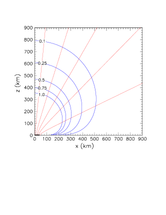
Figure 5: Streamlines and surfaces of constant $\omega_{\bf x}/\mu_{\bf x}$ for neutrinos emitted by an accretion disk with radius $R=50$ km. The surfaces are marked with the value of the $\nu_{e}$ survival probability, assuming the adiabatic limit of collective oscillations.

For purposes of illustration we now consider an explicit example for a disk-like source. Following the numerical studies of Ruffert and Janka Ruffert:1998qg for coalescing neutron stars, we use the following parameters for a disk source as an extremely schematic model. The all-species neutrino luminosity of the models shown by Ruffert and Janka varies between $(1-12)\times 10^{52}~{}{\rm erg}~{}{\rm s}^{-1}$ and the luminosity in species other than $\nu_{e}$ and $\bar{\nu}_{e}$ is always very small. Typically $\langle E_{\nu_{e}}\rangle<\langle E_{\bar{\nu}_{e}}\rangle$, a typical average being 12 MeV that we will use for both species. In contrast to the SN case, here one expects an excess of the ${\bar{\nu}}_{e}$ number flux over $\nu_{e}$, so that in this case we normalize the polarization vectors to the antineutrino flux. The ratio of number fluxes $\alpha=F_{\nu_{e}}/F_{\bar{\nu}_{e}}$ varies between about 0.65 and 0.81 if we ignore one case where the number fluxes are exactly equal and one where the $\nu_{e}$ flux practically vanishes.

Inspired by these numbers and the pictures shown by Ruffert and Janka we adopt the following parameters for our homogeneous disk-like neutrino source: Radius $R=50$ km, $L_{\bar{\nu}_{e}}=3\times 10^{52}~{}{\rm erg}~{}{\rm s}^{-1}$, $\langle E_{\nu}\rangle=12$ MeV, and $\alpha=0.75$. This implies a $\bar{\nu}_{e}$ flux at the disk of $F_{0}=2.0\times 10^{43}~{}{\rm cm}^{-2}~{}{\rm s}^{-1}$ and a scale for the neutrino-neutrino interaction strength of $\mu_{0}=\sqrt{2}G_{\rm F}F_{0}=8.4\times 10^{-5}~{}{\rm eV}=4.3\times 10^{5}~{}{\rm km}^{-1}$. We have in mind two-flavor oscillations driven by the atmospheric neutrino mass difference for which we use $\Delta m^{2}_{\rm atm}=2.4\times 10^{-3}~{}{\rm eV}^{2}$. Then the average vacuum oscillation frequency is $\omega_{0}=\langle\Delta m^{2}_{\rm atm}/2E\rangle=1.50\times 10^{-10}~{}{\rm eV}=0.76~{}{\rm km}^{-1}$. Here we have used that for an average neutrino energy $\langle E\rangle=12$ MeV and assuming a Maxwell-Boltzmann spectrum we have $\langle 1/E\rangle=1/(8~{}{\rm MeV})$.

The transition between the synchronized and the bipolar oscillation region, where the flavor pendulum begins to nutate and neutrino transformations begin in earnest, occurs at Hannestad:2006nj

$$\frac{\omega_{\bf x}}{\mu_{\bf x}}\approx\frac{(1-\sqrt{\alpha})^{2}}{2}\,,$$ (40)

which is $9\times 10^{-3}$ for $\alpha=0.75$ in this scenario.

In Fig. 5 we show the contours of constant $\omega_{\bf x}/\mu_{\bf x}$, which are the same as those of constant $P_{ee}$ under adiabatic approximation, for inverted hierarchy. The contour with $P_{ee}=1.0$ is the one where the condition of Eq. (40) occurs and the synchronized to bipolar transition takes place. Within the region enclosed by this contour, the oscillations are strongly synchronized so that macroscopically nothing much happens. This contour delineates the area where the flavor survival probability is essentially unity for both $\nu_{e}$ and $\bar{\nu}_{e}$. Outside this region, neutrino transitions begin and we show contours of the $\nu_{e}$ survival probability that indicates to which extent the initial $\nu_{e}$ and $\bar{\nu}_{e}$ fluxes have been converted to other flavors.

For our specific numerical example, we find that collective neutrino flavor conversions start at $z\gtrsim 400$ km. Since the $\nu_{e}{\bar{\nu}}_{e}$ annihilation rate per unit volume decreases very rapidly far from the source (for a spherical geometry one would expect $\sim r^{-8}$ goodman ) we do not expect that these flavor transitions affect significantly the neutrino energy deposition rate in the plasma. However, the features of neutrino fluxes emitted from coalescing neutron stars are rather model dependent. Here we speculate that if the asymmetry between the emitted neutrino species would be smaller, one could have collective flavor conversion or perhaps some sort of kinematical decoherence of the neutrino ensemble in a region close to the source, with a possible impact on the annihilation rate. We also note that the matter density in the region close to the source is expected to be $\rho\sim 10^{10-12}~{}{\rm g~{}cm}^{-3}$, thus it is so strong to prevent ordinary resonant flavor conversions Volkas:1999gb . At larger distance one expects that two resonant level crossings will occur. However, due to the uncertainties of the matter density profile in these regions, it is difficult to predict their effects on the neutrino burst.

VI Conclusions

Neutrinos streaming from powerful astrophysical sources such as SN cores or coalescing neutron stars are so dense near the source that they must show nonlinear flavor oscillations induced by the neutrino-neutrino refractive effect. Numerical simulations reveal a rich variety of phenomena, some of which have been explained with simple analytic models. However, numerical simulations thus far have been restricted to homogeneous gases evolving in time or to sources with exact spherical symmetry. More general geometries are numerically much more demanding and have not yet been studied.

Therefore, we have studied what might be expected under the assumption that the multi-angle instability plays no role and that the neutrino ensemble is largely characterized by self-maintained coherence. In this case one is led to a unique formulation of the collective equations of motion that imply that collective flavor oscillations should be thought of as a one-dimensional phenomenon along the streamlines of the underlying neutrino flux. Close to the source these streamlines are usually curved even though, of course, the underlying neutrino trajectories are straight. (We have neglected the gravitational bending of trajectories.) Therefore, even if the neutrino stream has no global symmetries, the collective oscillation problem is relatively simple.

We have used the concept of “self-maintained coherence” in the most restrictive sense that applies when the neutrino gas is dense, i.e., when a typical neutrino-neutrino interaction energy $\mu$ is large compared to a typical vacuum oscillation frequency $\omega_{0}=\langle\Delta m^{2}/2E\rangle$. The neutrino ensemble in this case evolves along a streamline as one unit that previously has been described as a gyroscopic pendulum in flavor space. All neutrino and anti-neutrino polarization vectors point essentially in the same direction in flavor space, the pendulum direction, allowing for the simplifications that lead to our collective equations. We have provided a prescription for defining the effective neutrino-neutrino interaction strength $\mu$ that works for general source geometries. Our result is somewhat different from what was used in the previous literature, but our expression for $\mu$ agrees better with numerical simulations.

There are more general forms of collective behavior. In a homogeneous isotropic system with a density that decreases adiabatically in time, the polarization vectors are at first aligned and stay in a single co-rotating plane even when $\mu$ becomes of order $\omega_{0}$ and smaller. However, they will align or anti-align themselves in the mass direction, leading to the phenomenon of spectral splits. This is a more general case of self-maintained coherence beyond our simple picture and is analytically fully understood. In the spherically symmetric case, numerical multi-angle simulations show a similar behavior. If the asymmetry between neutrinos and antineutrinos is large enough to prevent multi-angle decoherence, the neutrino and antineutrino modes evolve collectively essentially along the co-rotating plane, but with intriguing three-dimensional patterns that evolve collectively and are stable in flavor space. Once more spectral splits develop, similar to the single-angle approximation.

We speculate that these more general forms of behavior also occur for more general source geometries if we follow the neutrino stream lines. It is clear that multi-angle decoherence will occur if the asymmetry between neutrinos and anti-neutrinos is extremely small. Even a few per cent asymmetry, on the other hand, implies that close to the source we have synchronized oscillations, or, in the pendulum picture, it precesses fast without nutations. Therefore, close to the source where the streamlines are curved, our treatment should be most appropriate. If the effective mixing angle is small (as it will be because of the presence of ordinary matter), superficially no flavor oscillations happen close to the source and the “true action” begins at the synchronization radius where the inverted pendulum begins to nutate and begins to lose its initial orientation. If this point is reached at some distance, the streamlines will essentially point straight away from the source and naively one should think that henceforth the evolution is similar to the spherically symmetric case. In fact in the adiabatic approximation, one only needs to know the local value of $\omega_{0}/\mu$ in order to determine the neutrino survival probabilities, for any source geometry.

Granting these assumptions, we have briefly studied a toy model for coalescing neutron stars where the source is taken to be a homogeneously radiating disk. For our numerical example, we find that the region where collective oscillations will convert the original $\nu_{e}$ and ${\bar{\nu}_{e}}$ fluxes is quite far from the emission surface. Therefore these flavor conversions should have a negligible effect on the neutrino energy deposition in the plasma. However, due to the uncertainties of the original neutrino fluxes, we can not exclude situations with a smaller asymmetry between the original fluxes. Such tiny neutrino asymmetries may give rise to multi-angle decoherence, that could produce significant flavor conversions near the emitting disk. This question ultimately will need to be addressed numerically by means of large-scale numerical simulations of neutrino flavor evolution near a non-spherical source, in analogy to what has been done in the case of neutrinos streaming off a SN core.

Our study suggests that self-maintained coherence among different neutrino modes may well be a typical form of behavior even in non-spherical systems and notably in the interesting case of coalescing neutron stars. The final verdict on the role of collective neutrino oscillations in such systems can only come from numerical studies. At very least, our approach provides a simple limiting case against which one can measure the output of numerical simulations.

Appendix A Disk source

We here briefly describe the numerical integrations for a disk source that were used in the main text. The direction of neutrino momenta are determined by two polar angles $\theta_{p}$ and $\phi_{p}$, by which we can express the component of the neutrino velocity in $x$ and $z$ direction respectively by

$$v^{x} = \cos\phi_{p}\sin\theta_{p}\,,$$

$$v^{z} = \cos\theta_{p}\,.$$ (41)

Our first task is to determine the flux ${\bf F}_{\bf x}$, i.e., the $x$ and $z$ components $F^{x}_{x,z}$ and $F^{z}_{x,z}$, each as a function of $x$ and $z$. These are given by

$$F^{x}_{x,z} = \frac{1}{8\pi^{3}}\int{\rm d}E\,{\rm d}\cos\theta_{p}\,{\rm d}\phi_{p}v^{x}f_{x,z}(v^{x},v^{z})\,,$$

$$F^{z}_{x,z} = \frac{1}{8\pi^{3}}\int{\rm d}E\,{\rm d}\cos\theta_{p}\,{\rm d}\phi_{p}v^{z}f_{x,z}(v^{x},v^{z})\,.$$ (42)

One can also define the local neutrino density

$$n_{x,z}=\frac{1}{8\pi^{3}}\int{\rm d}E{\rm d}\cos\theta_{p}{\rm d}\phi_{p}f_{x,z}(v^{x},v^{z})\,\ .$$ (43)

In the case of synchronization, from Eq. (21) we arrive at the following EOM

$$(\langle v^{x}_{x,z}\rangle\partial_{x}+\langle v^{z}_{x,z}\rangle\partial_{z})a_{x,z}=\omega_{0}\,\ ,$$ (44)

where

$$\langle v^{x}_{x,z}\rangle = \frac{F^{x}_{x,z}}{n_{x,z}}\,\ ,$$

$$\langle v^{z}_{x,z}\rangle = \frac{F^{z}_{x,z}}{n_{x,z}}\,\ .$$ (45)

In this case, we have obtained a first order partial differential equation (PDE). Since $\langle v^{x}_{x,z}\rangle$ and $\langle v^{z}_{x,z}\rangle$ are not constant, in this case the streamlines will be curved. If the streamlines are graphs of the function $z(x)$, it follows

$$\frac{{\rm d}z}{{\rm d}x}=\frac{\langle v^{z}_{x,z}\rangle}{\langle v^{x}_{x,z}\rangle}\,\ ,$$ (46)

(i.e., the tangent line to the graph of $z(x)$ at $(x,z)$ is parallel to ${\bf v}$.) The ordinary differential equation (ODE) in Eq. (46) is the so-called characteristic equation for the associated PDE. Its solutions are the streamlines for the PDE.

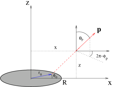
Figure 6: Relation between the momenta variables $\theta_{p}$ and $\phi_{p}$ and coordinates $r_{0}$ and $\phi_{0}$ on the disk.

The range of the previous angular integrations are determined by the coordinates $x$ and $z$. It could be convenient to express the previous integrals at a given point, writing $\theta_{p}$ and $\phi_{p}$ in terms of the coordinates $r_{0}$ and $\phi_{0}$ on the disk, by tracing back the direction of neutrino momenta on the disk, as shown in Fig. 6. Let the neutrino emitted from a point $(r_{0}\cos\phi_{0},r_{0}\sin\phi_{0},0)$ pass through the location $(x,0,z)$. The direction of the momentum of this neutrino is along the unit vector $(\sin\theta_{p}\cos\phi_{p},\sin\theta_{p}\sin\phi_{p},\cos\theta_{p})$. Therefore,

$$(x-r_{0}\cos\phi_{0},-r_{0}\sin\phi_{0},z)\propto\phantom{morespace}$$

$$\phantom{space}(\sin\theta_{p}\cos\phi_{p},\sin\theta_{p}\sin\phi_{p},\cos\theta_{p})\;.$$ (47)

We can now write down $\theta_{p}$ and $\phi_{p}$ explicitly in terms of $r_{0},\phi_{0},x,z$:

$$\tan\theta_{p}=\frac{\sqrt{r_{0}^{2}+x^{2}-2xr_{0}\cos\phi_{0}}}{z}\;,$$ (48)

so that

$$\cos\theta_{p} = \frac{z}{\sqrt{r_{0}^{2}+x^{2}-2xr_{0}\cos\phi_{0}+z^{2}}}\,\ ,$$

$$\sin\theta_{p} = \frac{\sqrt{r_{0}^{2}+x^{2}-2xr_{0}\cos\phi_{0}}}{\sqrt{r_{0}^{2}+x^{2}-2xr_{0}\cos\phi_{0}+z^{2}}}\;.$$ (49)

For the angle $\phi_{p}$, we get

$$\sin\phi_{p} = -\frac{r_{0}\sin\phi_{0}}{\sin\theta_{p}}=-\frac{r_{0}\sin\phi_{0}}{z\tan\theta_{p}}\,\ ,$$

$$\cos\phi_{p} = \frac{x-r_{0}\cos\phi_{0}}{\sin\theta_{p}}=\frac{x-r_{0}\cos\phi_{0}}{z\tan\theta_{p}}\,\ ,$$ (50)

so that

$$\phi_{p}=-\arctan\left(\frac{r_{0}\sin\phi_{0}}{x-r_{0}\cos\phi_{0}}\right)\,\ .$$ (51)

Using as variables of integration $r_{0}$ and $\phi_{0}$, we obtain

$$n_{x,z} = \int\frac{{\rm d}E}{8\pi^{3}}{\rm d}\cos\theta_{p}{\rm d}\phi_{p}f_{x,z}(v^{x},v^{z})$$ (52)

$$= \int{\rm d}r_{0}{\rm d}\phi_{0}\textrm{det}J(r_{0},\phi_{0}){\tilde{f}}_{x,z}(v^{x},v^{z})\,\ ,$$

where $J(r_{0},\phi_{0})$ is the Jacobian that relates the two coordinate systems, and $0\leq r_{0}\leq 1$ and $0\leq\phi_{0}\leq 2\pi$.

The derivatives relevant for the Jacobian are the following

$$\frac{\partial\cos\theta_{p}}{\partial r_{0}} = \frac{-z(r_{0}-x\cos\phi_{0})}{(r_{0}^{2}+x^{2}-2xr_{0}\cos\phi_{0}+z^{2})^{3/2}}\,\ ,$$

$$\frac{\partial\cos\theta_{p}}{\partial\phi_{0}} = \frac{-zxr_{0}\sin\phi_{0}}{(r_{0}^{2}+x^{2}-2xr_{0}\cos\phi_{0}+z^{2})^{3/2}}\,\ ,$$

$$\frac{\partial\phi_{p}}{\partial r_{0}} = -\frac{x\sin\phi_{0}}{r_{0}^{2}+x^{2}-2xr_{0}\cos\phi_{0}}\,\ ,$$

$$\frac{\partial\phi_{p}}{\partial\phi_{0}} = \frac{r_{0}^{2}-xr_{0}\cos\phi_{0}}{r_{0}^{2}+x^{2}-2xr_{0}\cos\phi_{0}}\,\ ,$$ (53)

so that

$$\textrm{det}J = \frac{\partial\cos\theta_{p}}{\partial r_{0}}\frac{\partial\phi_{p}}{\partial\phi_{0}}-\frac{\partial\cos\theta_{p}}{\partial\phi_{0}}\frac{\partial\phi_{p}}{\partial r_{0}}$$ (54)

$$= \frac{-zr_{0}}{(r_{0}^{2}+x^{2}-2xr_{0}\cos\phi_{0}+z^{2})^{3/2}}\;.$$

The net result is

$$F^{x}_{x,z} = \int\frac{{\rm d}E}{8\pi^{3}}{\rm d}\phi_{0}{\rm d}r_{0}\frac{-zr_{0}(x-r_{0}\cos\phi_{0})f_{x,z}(v^{x},v^{z})}{(r_{0}^{2}+x^{2}-2xr_{0}\cos\phi_{0}+z^{2})^{2}}\,\ ,$$

$$F^{z}_{x,z} = \int\frac{{\rm d}E}{8\pi^{3}}{\rm d}\phi_{0}{\rm d}r_{0}\frac{z(-zr_{0})f_{x,z}(v^{x},v^{z})}{(r_{0}^{2}+x^{2}-2xr_{0}\cos\phi_{0}+z^{2})^{2}}\,\ .$$

References

- (1) J. Pantaleone, “Neutrino oscillations at high densities,” Phys. Lett. B 287, 128 (1992).
- (2) G. Sigl and G. Raffelt, “General kinetic description of relativistic mixed neutrinos,” Nucl. Phys. B 406, 423 (1993).
- (3) S. Samuel, “Neutrino oscillations in dense neutrino gases,” Phys. Rev. D 48, 1462 (1993).
- (4) V. A. Kostelecký and S. Samuel, “Neutrino oscillations in the early universe with an inverted neutrino mass hierarchy,” Phys. Lett. B 318, 127 (1993).
- (5) V. A. Kostelecký and S. Samuel, “Self-maintained coherent oscillations in dense neutrino gases,” Phys. Rev. D 52, 621 (1995) [hep-ph/9506262].
- (6) S. Samuel, “Bimodal coherence in dense selfinteracting neutrino gases,” Phys. Rev. D 53, 5382 (1996) [hep-ph/9604341].
- (7) S. Pastor, G. G. Raffelt and D. V. Semikoz, “Physics of synchronized neutrino oscillations caused by self-interactions,” Phys. Rev. D 65, 053011 (2002) [hep-ph/0109035].
- (8) Y. Y. Y. Wong, “Analytical treatment of neutrino asymmetry equilibration from flavour oscillations in the early universe,” Phys. Rev. D 66, 025015 (2002) [hep-ph/ 0203180].
- (9) K. N. Abazajian, J. F. Beacom and N. F. Bell, “Stringent constraints on cosmological neutrino antineutrino asymmetries from synchronized flavor transformation,” Phys. Rev. D 66, 013008 (2002) [astro-ph/0203442].
- (10) S. Pastor and G. Raffelt, “Flavor oscillations in the supernova hot bubble region: Nonlinear effects of neutrino background,” Phys. Rev. Lett. 89, 191101 (2002) [astro-ph/0207281].
- (11) R. F. Sawyer, “Classical instabilities and quantum speed-up in the evolution of neutrino clouds,” hep-ph/0408265.
- (12) R. F. Sawyer, “Speed-up of neutrino transformations in a supernova environment,” Phys. Rev. D 72, 045003 (2005) [hep-ph/0503013].
- (13) R. F. Sawyer, “The multi-angle instability in dense neutrino systems,” arXiv:0803.4319 [astro-ph].
- (14) H. Duan, G. M. Fuller and Y. Z. Qian, “Collective neutrino flavor transformation in supernovae,” Phys. Rev. D 74, 123004 (2006) [astro-ph/0511275].
- (15) H. Duan, G. M. Fuller, J. Carlson and Y. Z. Qian, “Simulation of coherent non-linear neutrino flavor transformation in the supernova environment. I: Correlated neutrino trajectories,” Phys. Rev. D 74, 105014 (2006) [astro-ph/0606616].
- (16) S. Hannestad, G. G. Raffelt, G. Sigl and Y. Y. Y. Wong, “Self-induced conversion in dense neutrino gases: Pendulum in flavor space,” Phys. Rev. D 74, 105010 (2006); Erratum ibid. 76, 029901 (2007) [astro-ph/0608695].
- (17) G. G. Raffelt and G. Sigl, “Self-induced decoherence in dense neutrino gases,” Phys. Rev. D 75, 083002 (2007) [hep-ph/0701182].
- (18) H. Duan, G. M. Fuller, J. Carlson and Y. Z. Qian, “Analysis of collective neutrino flavor transformation in supernovae,” Phys. Rev. D 75, 125005 (2007) [astro-ph/0703776].
- (19) G. G. Raffelt and A. Yu. Smirnov, “Self-induced spectral splits in supernova neutrino fluxes,” Phys. Rev. D 76, 081301 (2007); Erratum ibid. 77, 029903 (2008) [arXiv:0705.1830 (hep-ph)].
- (20) G. G. Raffelt and A. Yu. Smirnov, “Adiabaticity and spectral splits in collective neutrino transformations,” Phys. Rev. D 76, 125008 (2007) [arXiv:0709.4641 (hep-ph)].
- (21) A. Esteban-Pretel, S. Pastor, R. Tomàs, G. G. Raffelt and G. Sigl, “Decoherence in supernova neutrino transformations suppressed by deleptonization,” Phys. Rev. D 76, 125018 (2007) [arXiv:0706.2498 (astro-ph)].
- (22) H. Duan, G. M. Fuller and Y. Z. Qian, “A simple picture for neutrino flavor transformation in supernovae,” Phys. Rev. D 76, 085013 (2007) [arXiv:0706.4293 (astro-ph)].
- (23) H. Duan, G. M. Fuller, J. Carlson and Y.Z. Qian, “Neutrino mass hierarchy and stepwise spectral swapping of supernova neutrino flavors,” Phys. Rev. Lett. 99, 241802 (2007) [arXiv:0707.0290 (astro-ph)].
- (24) G. L. Fogli, E. Lisi, A. Marrone and A. Mirizzi, “Collective neutrino flavor transitions in supernovae and the role of trajectory averaging,” JCAP 0712, 010 (2007) [arXiv:0707.1998 (hep-ph)].
- (25) H. Duan, G. M. Fuller, J. Carlson and Y. Z. Qian, “Flavor evolution of the neutronization neutrino burst from an O-Ne-Mg core-collapse supernova,” Phys. Rev. Lett. 100, 021101 (2008) [arXiv:0710.1271 (astro-ph)].
- (26) B. Dasgupta, A. Dighe, A. Mirizzi and G. G. Raffelt, “Spectral split in prompt supernova neutrino burst: Analytic three-flavor treatment,” arXiv:0801.1660 [hep-ph].
- (27) A. Esteban-Pretel, S. Pastor, R. Tomàs, G. G. Raffelt and G. Sigl, “Mu-tau neutrino refraction and collective three-flavor transformations in supernovae,” Phys. Rev. D 77, 065024 (2008) [arXiv:0712.1137 (astro-ph)].
- (28) B. Dasgupta and A. Dighe “Collective three-flavor oscillations of supernova neutrinos,” [arXiv:0712.3798 (hep-ph)].
- (29) H. Duan, G. M. Fuller and Y. Z. Qian, “Stepwise spectral swapping with three neutrino flavors,” Phys. Rev. D 77, 085016 (2008) [arXiv:0801.1363 (hep-ph)].
- (30) B. Dasgupta, A. Dighe and A. Mirizzi, “Identifying neutrino mass hierarchy at extremely small theta(13) through Earth matter effects in a supernova signal,” arXiv:0802.1481 [hep-ph].
- (31) H. Duan, G. M. Fuller and J. Carlson, “Simulating nonlinear neutrino flavor evolution,” arXiv:0803.3650 [astro-ph].
- (32) M. Ruffert and H.-T. Janka, “Gamma-ray bursts from accreting black holes in neutron star mergers,” Astron. Astrophys. 344, 573 (1999) [astro-ph/9809280].
- (33) A. D. Dolgov, “Neutrinos in the early universe,” Yad. Fiz. 33, 1309 (1981) [Sov. J. Nucl. Phys. 33, 700 (1981)].
- (34) M. A. Rudzsky, “Kinetic equations for neutrino spin- and type-oscillations in a medium,” Astrophys. Space Science 165, 65 (1990).
- (35) B. H. J. McKellar and M. J. Thomson, “Oscillating doublet neutrinos in the early universe,” Phys. Rev. D 49, 2710 (1994).
- (36) P. Strack and A. Burrows, “A generalized Boltzmann formalism for oscillating neutrinos,” Phys. Rev. D 71, 093004 (2005) [hep-ph/0504035].
- (37) C. Y. Cardall, “Liouville equations for neutrino distribution matrices,” arXiv:0712.1188 [astro-ph].
- (38) S. Mrowczynski and M. H. Thoma, “What do electromagnetic plasmas tell us about quark-gluon plasma?,” Ann. Rev. Nucl. Part. Sci. 57, 61 (2007) [nucl-th/0701002].
- (39) E. C. Zachmanoglou and D. W. Thoe, Introduction to Partial Differential Equations with Applications (Dover Publications, New York, 1986).
- (40) J. Goodman, A. Dar, and S. Nussinov, “Neutrino annihilation in Type II supernovae,” Astrophys. J. Lett. 314, L7 (1987).
- (41) R. R. Volkas and Y. Y. Y. Wong, “Matter-affected neutrino oscillations in ordinary and mirror stars and their implications for gamma-ray bursts,” Astropart. Phys. 13, 21 (2000) [astro-ph/9907161].