Electromagnetic energy flow lines as possible paths of photons

Abstract

Motivated by recent experiments where interference patterns behind a grating are obtained by accumulating single photon events, here we provide an electromagnetic energy flow-line description to explain the emergence of such patterns. We find and discuss an analogy between the equation describing these energy flow lines and the equation of Bohmian trajectories used to describe the motion of massive particles.

,, ,,

1 Introduction

The possibility of performing quantum interference experiments with low-intensity beams (i.e., one per one particle) of photons [1, 2, 3] and material particles [4, 5, 6] has intensified the theoretical search of the topology of the photon paths [7, 8, 9] and particle trajectories [10, 11, 12, 13, 14] that describe the process behind the interference grating. The aim of all the proposed approaches is to simulate the appearance of the interference pattern by accumulation of single-particle events.

In Bohmian mechanics one may simulate this process for material particles. Bohmian trajectories follow the streamlines associated with the quantum-mechanical probability current density and, therefore, reproduce exactly the quantum-mechanical particle space distribution in both the near and the far fields [10, 11, 12]. Alternatively, the emergence of the interference pattern in the far field has also been simulated by sets of rectilinear trajectories characterized by the momentum distribution associated with the particle wave function [13, 14]. In the far field, the distribution of momentum components along Bohmian trajectories is consistent with this distribution [14].

In this paper, we show how to determine electromagnetic energy (EME) flow lines behind an interference grating, where the components of the magnetic and electric vector fields satisfy Maxwell’s equations. These fields are expressed in terms of a function which explicitly takes into account the boundary conditions imposed by the grating. The EME flow lines are then determined after numerically solving the path equation arising from the Poynting energy flow vector. In particular, here we show EME flow lines behind gratings consisting of different number of slits. These sets of lines supplement those presented by Prosser [7] for both a semi-infinite plane and gratings with one and two slits. The EME flow lines show that the energy redistribution behind the grating until reaching the Fraunhofer regime. In particular, it is of interest the process that corresponds to multiple-slit gratings, where we can observe the smooth transition from a Talbot pattern in the near field to the characteristic Fraunhofer peaks in the far field.

It is tempting to conclude from the results obtained that the motion of an eventual photon wave packet thus represents an energy flow along a group of flow lines. This conclusion is supported also by the fact that the path equation for the EME flow lines has the same form as the equation for the quantum flow associated with material particles. This explains why there is a complete similarity in interference phenomena with photons and material particles. Experimentally, the final interference patterns as well as the processes of their emergence are analogous [1, 2, 3, 4, 5, 6].

2 The complex Poynting vector and the equation for the EME flow lines

The diffraction of electromagnetic radiation by a grating is described by the solution of Maxwell’s equations in vacuum that satisfy the grating boundary conditions [15]. We consider the simplest solutions of Maxwell’s equations: harmonic electromagnetic waves

$$\tilde{\bf H}({\bf r},t) = {\bf H}({\bf r})e^{-i\omega t},$$ (1)

$$\tilde{\bf E}({\bf r},t) = {\bf E}({\bf r})e^{-i\omega t}.$$ (2)

The physical electric and magnetic fields are obtained by taking the real parts of the corresponding complex quantities. The space-dependent parts of these fields (which are complex amplitudes) satisfy the time-independent Maxwell equations

$$\nabla\times{\bf H}({\bf r}) = -i\omega\epsilon_{0}{\bf E}({\bf r}),$$ (3)

$$\nabla\times{\bf E}({\bf r}) = i\omega\mu_{0}{\bf H}({\bf r}),$$ (4)

$$\nabla\cdot{\bf H}({\bf r}) = 0,$$ (5)

$$\nabla\cdot{\bf E}({\bf r}) = 0.$$ (6)

From these equations it follows that both fields, ${\bf E}({\bf r})$ and ${\bf H}({\bf r})$, satisfy the Helmholtz equation

$$\nabla^{2}{\bf H}({\bf r})+k^{2}{\bf H}({\bf r}) = 0,$$ (7)

$$\nabla^{2}{\bf E}({\bf r})+k^{2}{\bf E}({\bf r}) = 0,$$ (8)

where $k=\omega/c$.

The EME flow lines are now determined from the energy flux vector, which is the time-averaged flux of energy, given by the real part of the complex Poynting vector [16]

$${\bf S}({\bf r})=\frac{1}{2}\ \!{\rm Re}[{\bf E}({\bf r})\times{\bf H}^{*}({\bf r})].$$ (9)

Note that, since the flow of energy goes in the direction of the Poynting vector, the EME flow lines can then be determined from the parametric differential equation

$$\frac{d{\bf r}}{ds}=\frac{1}{c}\frac{{\bf S}({\bf r})}{U({\bf r})},$$ (10)

were $s$ is a certain arc-length along the corresponding path and $U({\bf r})$ is the time-averaged electromagnetic energy density

$$U({\bf r})=\frac{1}{4}\ \![\epsilon_{0}{\bf E}({\bf r})\cdot{\bf E}^{*}({\bf r})+\mu_{0}{\bf H}({\bf r})\cdot{\bf H}^{*}({\bf r})].$$ (11)

3 The Poynting vector in the case of two dimensional diffraction by a plane grating

To describe simple diffraction experiments, we will consider that the grating is on the $XZ$ plane at $y=0$, with the incident plane harmonic wave traveling along the $y$-direction. Moreover, we assume the problem to be completely independent of the $z$-coordinate (i.e., very long slits along this coordinate). In order to encompass all possible cases of polarization, we express the magnetic and electric fields before the grating as a superposition of two waves: $H$ polarized, for which the magnetic field is along $z$ ($A$ components), and $E$ polarized, for which the electric field is along $z$ ($B$ components) [17]. That is,

$$\tilde{\bf H}({\bf r},t) = {\bf H}({\bf r})e^{-i\omega t}=\left[Ae^{iky}{\bf e}_{z}+Be^{i\phi}e^{iky}{\bf e}_{x}\right]e^{-i\omega t},$$ (12)

$$\tilde{\bf E}({\bf r},t) = {\bf E}({\bf r})e^{-i\omega t}=\frac{k}{\epsilon_{0}\omega}\left[-Ae^{iky}{\bf e}_{x}+Be^{i\phi}e^{iky}{\bf e}_{z}\right]e^{-i\omega t}.$$ (13)

Here, $\phi$ is the phase shift between the $x$-and $z$-component of the field, and the constants $A$ and $B$ are real. For $\phi=0$ or $\pi$, the incident wave is linearly polarized, while the cases $A=B$, with $\phi=\pm\pi/2$, describe circular polarization. The cases $A\neq B$, with $\phi\neq 0,\pi$ and $\pm\pi/2$, describe elliptic polarization.

As shown by Born and Wolf [17], the $E$-polarization and $H$-polarization components satisfy two independent sets of equations since the problem is independent of the $z$-coordinate. This implies that the solution that corresponds to an incident wave, given by (12) and (13), diffracted by a grating can be expressed as

$${\bf H} = ik^{-1}Be^{i\phi}\ \!\frac{\partial\psi}{\partial y}\ \!{\bf e}_{x}-ik^{-1}Be^{i\phi}\ \!\frac{\partial\psi}{\partial x}\ \!{\bf e}_{y}+A\psi\ \!{\bf e}_{z},$$ (14)

$${\bf E} = \frac{iA}{\epsilon_{0}\omega}\frac{\partial\psi}{\partial y}\ \!{\bf e}_{x}-\frac{iA}{\epsilon_{0}\omega}\frac{\partial\psi}{\partial x}\ \!{\bf e}_{y}+\frac{kB}{\epsilon_{0}\omega}\ \!e^{i\phi}\psi\ \!{\bf e}_{z},$$ (15)

where $\psi(x,y)$ is a solution of the Helmholtz equation

$$\nabla^{2}\psi+k^{2}\psi=0,$$ (16)

which satisfies the grating boundary conditions. From (14) and (15), we can now express the components of the time-averaged Poynting vector in terms of the constants $A$, $B$ and $\phi$ and the function $\psi(x,y)$, as

$$S_{x} = \frac{i}{4\epsilon_{0}\omega}\ \!(A^{2}+B^{2})\left(\psi\frac{\partial\psi^{*}}{\partial x}-\psi^{*}\frac{\partial\psi}{\partial x}\right),$$ (17)

$$S_{y} = \frac{i}{4\epsilon_{0}\omega}\ \!(A^{2}+B^{2})\left(\psi\frac{\partial\psi^{*}}{\partial y}-\psi^{*}\frac{\partial\psi}{\partial y}\right),$$ (18)

$$S_{z} = \frac{i}{2\epsilon_{0}\omega k}\ \!AB\sin\phi\left(\frac{\partial\psi}{\partial x}\frac{\partial\psi^{*}}{\partial y}-\frac{\partial\psi^{*}}{\partial x}\frac{\partial\psi}{\partial x}\right).$$ (19)

In the case of a linearly polarized initial wave ($\phi=0$ or $\pi$), it follows from equation (19) that the $z$ component of the Poynting vector vanishes. Thus, the EME flow lines will remain confined on the $XY$ plane and, from the parametric differential equation (10), we find that the differential equation

$$\frac{dy}{dx}=\frac{S_{y}}{S_{x}}=\frac{\displaystyle\left(\psi\frac{\partial\psi^{*}}{\partial y}-\psi^{*}\frac{\partial\psi}{\partial y}\right)}{\displaystyle\left(\psi\frac{\partial\psi^{*}}{\partial x}-\psi^{*}\frac{\partial\psi}{\partial x}\right)}$$ (20)

will determine the eventual photon paths, which are obtained by numerical integration. As can be noticed, the topology of the EME flow lines in the case of linear polarization is independent of the constants $A$ and $B$, and therefore independent of the direction of polarization.

On the other hand, for circular and elliptic polarizations the $z$-component of the Poynting vector is non zero, this leading to important differences in the properties of the corresponding EME flow lines, which will not be planar, as infers from the non vanishing $z$-component in equation (10). The properties of EME flow lines in these cases are beyond the scope of the present work and will be explored in a forthcoming one.

4 Flow lines behind a specific grating

In order to plot flow lines for a specific grating we need explicit expressions for the magnetic and electric field behind a grating. Traditionally, explicit solutions have been written using the solution of the Helmholtz equation in the form of the Fresnel-Kirchhoff integral [17]. By making the appropriate approximations, the solution was then transformed into the expressions valid in the Fresnel and Fraunhofer regions, respectively. Talbot effect and Talbot-Laue effect were also explained [18] by making the appropriate approximations and transformations of the Fresnel-Kirchhoff integral.

If the $x$ component of the wave vector satisfies the relation $k\gg k_{x}$, the solution of the Helmholtz equation may also be expressed as a superposition of transverse modes (STM) of the field multiplied by an exponential function of the longitudinal coordinate [19]. As shown by Arsenović et al[20], this form is equivalent to the Fresnel-Kirchhoff integral. For an incident plane wave falling on the grating at $y=0$ and lying on the $XZ$ plane, the STM form of the solution reads as

$$\psi(x,y)=\frac{e^{iky}}{\sqrt{2\pi}}\int_{-\infty}^{\infty}c(k_{x})\ \!e^{ik_{x}x}e^{-ik_{x}^{2}y/2k}dk_{x},$$ (21)

where the function $c(k_{x})$ is determined by the incident wave and the grating boundary conditions as

$$c(k_{x})=\frac{1}{\sqrt{2\pi}}\int_{-\infty}^{\infty}\psi(x,0)\ \!e^{-ik_{x}x}dk_{x}.$$ (22)

Within the approximation $k\gg k_{x}$, one finds

$$\left\arrowvert\frac{\partial\psi}{\partial x}\right\arrowvert\ll\left\arrowvert\frac{\partial\psi}{\partial y}\right\arrowvert,\qquad\frac{\partial\psi}{\partial y}\approx ik\psi,$$ (23)

and, therefore, the EME density (11) becomes proportional to $|\psi(x,y)|^{2}$, i.e.,

$$U({\bf r})=\frac{1}{2}\ \!\mu_{0}(A^{2}+B^{2})|\psi(x,y)|^{2},$$ (24)

which is obtained from (14), (15) and (11).

Assuming that the grating is completely transparent inside the slits and completely absorbing outside them, we have that $\psi(x,0)=0$ for points outside the slit aperture and $\psi(x,0)=\psi_{in}(x,0)$ for the inside points, where $\psi_{in}(x,0)$ is the field component of the incident wave. In the case of an incident plane wave propagating along the $y$-axis, $\psi_{in}(x,0)$ is a constant. For a grating with $N$ apertures separated a distance $d$ and all with the same width $\delta$, a simple integration [19] renders

$$c(k_{x})=\frac{1}{\sqrt{2\pi}}\sqrt{\frac{\delta}{N}}\frac{\sin(k_{x}\delta/2)}{k_{x}\delta/2}\frac{\sin(Nk_{x}d/2)}{\sin(k_{x}d/2)}.$$ (25)

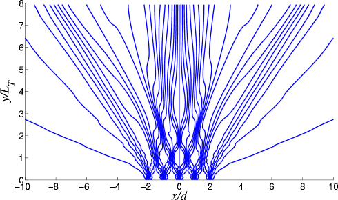
Figure 1: EME flow lines behind a Ronchi grating ($\delta=d/2$) with $N=5$ slits, $\lambda=500$ nm, $d=20\lambda=10$ $\mu$m and $L_{T}=d^{2}/\lambda=200$ $\mu$m.

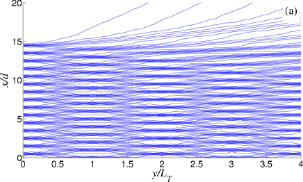
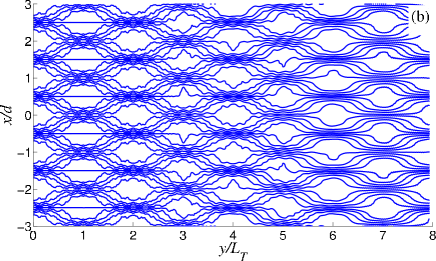
Figure 2: EME flow lines behind a Ronchi grating ($\delta=d/2$) with $N=30$ slits, $\lambda=500$ nm, $d=20\lambda=10$ $\mu$m and $L_{T}=d^{2}/\lambda=200$ $\mu$m. (a) EME lines from the upper part of the grating ($y>0$). (b) EME lines from six central slits of the grating.

In figures 1 and 2, we have represented the EME flow lines behind Ronchi gratings with 5 and 30 slits, respectively. The unit along the $y$-axis is the so-called Talbot distance, $\L_{T}=d^{2}/\lambda$, which gives the repetition period behind a grating of the diffracted wave [12]; the unit along the axis parallel to the grating ($x$-axis) is the period $d$ this grating. As seen, the topology displayed by the EME flow lines is very similar to that displayed by Bohmian trajectories for massive particles [10, 11, 12]. Note that the quantum density current

$${\bf J}=\frac{i\hbar}{2m}\ \!(\Psi\nabla\Psi^{*}-\Psi^{*}\nabla\Psi)$$ (26)

determines the particle trajectories in Bohmian mechanics through the equation of motion

$$\frac{d{\bf r}}{dt}=\frac{{\bf J}}{\rho},$$ (27)

where $\rho=\Psi^{*}\Psi$. The latter equation is analogous to equation (10), though this analogy is not totally complete: in the case of particles with a mass $m$, the relation $y=\hbar kt/m$ holds, whereas the same is not true for photons. When the wave function $\Psi$ does not depend on $z$, ${\bf J}$ has only $x$ and $y$ components,

$$J_{x}=\frac{i\hbar}{2m}\left(\Psi\frac{\partial\Psi^{*}}{\partial x}-\Psi^{*}\frac{\partial\Psi}{\partial x}\right)$$ (28)

$$J_{y}=\frac{i\hbar}{2m}\left(\Psi\frac{\partial\Psi^{*}}{\partial y}-\Psi^{*}\frac{\partial\Psi}{\partial y}\right).$$ (29)

Equations (28) and (29) have the same form as equations (17) and (18). Thus, the EME flow lines in the case of a linearly polarized incident wave are similar to the Bohmian trajectories of massive particles described by a two-dimensional wave function.

5 Emergence of the interference pattern by accumulation of single photon arrivals

In the case of massive particle the modulus square of the wave function describes the distribution of particles at a distance $y$ from the grating in the far field after (theoretically) an infinite number of particles has reached the detector (at $y$). This theoretical result has been nicely confirmed by a new generation of experiments which use low-intensity beams of particles. In these experiments, the final interference patterns are built-up after particles accumulate gradually one by one at a scanning screen [2, 3, 5, 6]. Numerical simulation of particle arrivals, assuming that they move along de Broglie-Bohm’s trajectories [10, 11, 12] and MD trajectories [13] describe theoretically this process. This means that a trajectory-based interpretation completes the standard interpretation of the wave function, where a picture in terms of single events is missing.

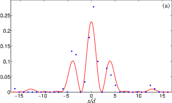
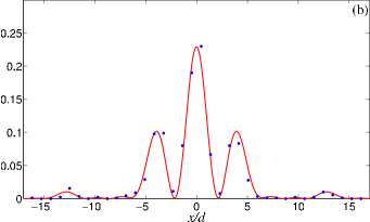
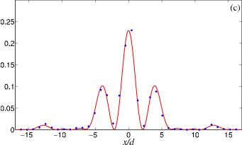
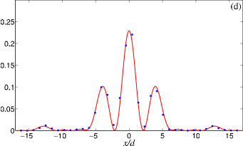
Figure 3: Histogram of the number of trajectories ending at various points along the $x$-axis at a distance $y=4.3L_{T}$ for four different values of the total number of photons: (a) 100, (b) 1000, (c) 2000 and (d) 5000. Here diffraction is produced by a two-slit grating and the initial conditions (positions along the two slits) for the photons data are chosen at random. The red line is the plot of the function $|\psi(x,y)|^{2}$. It is seen that at the chosen distance $y=4.3L_{T}$, maximum of the distribution at $x/d=8.6$, associated with $k_{x}d=4\pi$, is absent. This follows from (25) because for $N=2$, $d=2\delta$, the second interference maximum, being at $k_{x}d=4\pi$ coincides with the first diffraction minimum.

Analogously, one can proceed in the same way with photons assuming that they move along the EME flow lines described in the previous section. This is illustrated in figure 3, where we have plotted histograms (blue dots) obtained from the accumulation of photons for a two-slit diffraction experiment (with $\lambda=500$ nm, $d=20\lambda$ and $\delta=d/2$). In particular, the histograms have been made considering equally spaced bins (with a width of $0.9d$) at an observation distance $y_{ob}=4.3L_{T}$ from the plane of the grating, where the Fraunhofer pattern is already well converged (this happens when the observation distance is further away than the so-called Rayleigh distance [21], which in this case is $y_{R}\sim(2\delta+d/2)^{2}/4\pi\lambda\approx 0.2L_{T}\ll y_{ob}$). As can be seen, as we move from panel (a) to (d) the histogram data approach better and better the smooth (red) line which represents the EME density $U(x,y_{ob})$ given by equation (24) as the number of photons per time unit increases, as also seen in the experiment [2, 3]. It is interesting to note that the photons (or, equivalently, the initial positions of their paths) distribute randomly along the distance covered by each slit aperture and, therefore, their arrival positions at $y=4.3L_{T}$ will also be random. However, they will accumulate in accordance to $U({\bf r})$ because of the guidance condition given by equation (10), which can be alternatively expressed [17] as

$${\bf S}({\bf r})=U({\bf r}){\bf v},$$ (30)

where ${\bf v}$ is a sort of effective vectorial velocity field which transports the EME density through space in the form of the EME density current. The vector field ${\bf v}$ is always oriented in the direction of the wave vector ${\bf k}$. Thus, before the grating it is aligned along the $y$ direction and behind the grating will depend on the particular point $(x,y)$ where the field is evaluated, becoming almost constant along some specific direction only within the Fraunhofer regime.

References

References

-
[1]
Parker S 1971 Am. J. Phys. 39 420
Parker S 1972 Am. J. Phys. 40 1003 - [2] Dimitrova T L and Weis A 2008 Am. J. Phys. 76 137
- [3] http://ophelia.princeton.edu/page/single-photon.html
- [4] Rauch H and Werner S A 2000 Neutron Interferometry: Lessons in Experimental Quantum Mechanics (Oxford: Clarendon Press)
- [5] Tonomura A, Endo J, Matsuda T, Kawasaki T and Ezawa H 1989 Am. J. Phys. 57 117
- [6] Shimuzu F, Shimuzu K and Takuma H 1992 Phys. Rev. A 46 R17
-
[7]
Prosser R D 1976 Int. J. Theor. Phys. 15 169
Prosser R D 1976 Int. J. Theor. Phys. 15 181 - [8] Ghose P, Majumdar A S, Guha S and Sau J 2001 Phys. Lett. A 290 205
- [9] Holland P R 1993 The Quantum Theory of Motion (Cambridge: Cambridge University Press)
- [10] Sanz A S, Borondo F and Miret-Artés S 2002 J. Phys.: Condens. Matter 14 6109
- [11] Gondran M and Gondran A 2005 Am. J. Phys. 73 507
- [12] Sanz A S and Miret-Artés S 2007 J. Chem. Phys. 126 234106
- [13] Božić M and Arsenović D 2006 Acta Phys. Hung. B 26 219
- [14] Davidović M, Arsenović D, Božić M, Sanz A S and Miret-Artés S 2008 Eur. Phys. J. Spec. Top. 160 95
- [15] Sommerfeld A 1954 Lectures on Theoretical Physics vol 4 (New York: Academic Press)
- [16] Jackson J D 1998 Classical Electrodynamics 3rd ed (New York: Wiley)
- [17] Born M and Wolf E 2002 Principles of Optics 7th ed (expanded) (Oxford: Pergamon Press)
- [18] Clauser J F and Reinsch M W 1992 Appl. Phys. B 54 380
- [19] Arsenović D, Božić M and Vuškovic L 2002 J. Opt. B: Quantum Semiclass. Opt. 4 S358
- [20] Arsenović D, Božić M, Man’ko O V and Man’ko V I 2005 J. Russ. Laser Res. 26
- [21] Sanz A S, Borondo F and Miret-Artés S 2000 Phys. Rev. B 61 7743