1 Introduction

The LHC will be turned on soon. Excluding serendipitous events, it seems that signals will be seen only after complicated backgrounds have been properly subtracted out. Therefore, one must have a good account of the multi-particle processes, particularly those induced by QCD. Also, one should know the proper energy scale in a calculation to ensure stability relative to higher order effects. In other words, loops are also important, besides tree level results.

There has been much progress in perturbative evaluations [1], especially in the past few years [2, 3, 4, 5]. One would even venture to say that there is a new technology, which is applicable to all field theories. We shall confine our attention to QCD here.

If one is to follow the usual Feynman rules and diagrams to calculate a multi-gluon process, one will find that the algebra becomes horrendous very fast. For an $n$-gluon process at the tree level, if we just examine the three-point vertices, there are $n-2$ of them and each one has six terms which depend on some momenta, not to mention the internal symmetry coupling. Then one has to permute these $n$ legs over the vertices.

As we all know, a massless particle in four spacetime dimensions has at most two degrees of freedom, but a manifestly covariant formulation requires four components for a vector field. Therefore, there are tremendous amount of cancellations in the intermediate stage of a calculation to yield some simple looking final answer. The process somehow knows that the unphysical degrees of freedom should not be there and tries its best to expel them. Lots of efforts were wasted in the old ways. It will help if one eliminates all these unwanted degrees of freedom at an early stage in some way.

The new developments in non-Abelian gauge field calculations on the whole pursue two different paths, the ideas of which are not entirely new, but the executions are much improved:

(1) Using a physical gauge, such that there are explicitly only two components for each internal symmetry index.

(2) Using an extended dispersive technique, such that an $n$-point amplitude will be constructed from lower point on-shell physical amplitudes.

It turns out that these two methods can be made to complement each other and give rise to recursion relations for all the tree and some of the one-loop amplitudes [6]. For the other one-loop amplitudes with more complicated helicity composition, they are very much like the dispersion method using Cutkosky rules, but of course with much better handle and insight.

You must appreciate the possibility of having recursion relations, because one can recycle whatever hard work one has already put in to build up more complicated processes, rather than to start from the scratch all over again. This is possible, much to the credit of analytic continuation into complex momenta [5].

2 Spinors, Twistors and Complex Momenta

For a particle with zero mass, we can use two component spinors or twistors representation

$$P^{\dot{a}b}=(\tilde{\sigma}\cdot P)^{\dot{a}b}=|p]^{\dot{a}}<p|^{b},$$ (2.1)

and

$$P_{b\dot{a}}=(\sigma\cdot P)_{b\dot{a}}=|p>_{b}[p|_{\dot{a}}$$ (2.2)

where $\sigma^{\mu}=(-I,\vec{\sigma})$ and $\tilde{\sigma}^{\mu}=(-I,-\vec{\sigma})$. We use them to form scalar products of spinors

$$<p_{i}p_{j}>=<p_{i}|^{b}|p_{j}>_{b}=-<p_{j}p_{i}>,$$ (2.3)

and

$$[p_{j}p_{i}]=[p_{j}|_{\dot{a}}|p_{i}]^{\dot{a}}=-[p_{i}p_{j}],$$ (2.4)

from which the scalar product of two vectors is

$$-2P_{i}\cdot P_{j}=<p_{i}p_{j}>[p_{j}p_{i}].$$ (2.5)

Also, we use them to build polarization vectors for gauge particles of momentum $K_{i}$[7]

$$\epsilon^{h=+}(Q_{i},K_{i})^{\mu}={<q_{i}|\sigma^{\mu}|k_{i}]\over\sqrt{2}<q_{i}k_{i}>},\ \epsilon^{h=-}(Q_{i},K_{i})^{\mu}={[q_{i}|\tilde{\sigma}^{\mu}|k_{i}>\over\sqrt{2}[q_{i}k_{i}]}$$ (2.6)

in which $Q_{i}$ is a reference momentum, which can be individually assigned for each $K_{i}$. Changing $Q_{i}$ is a change of gauge.

For real momenta, we have

$$[p_{i}p_{j}]=<p_{j}p_{i}>^{\star},$$ (2.7)

which is a result we don’t like, if we want to perform on-shell calculation. Let us consider forming an amplitude for three on-shell gluons

$$P_{1}+P_{2}+P_{3}=0.$$ (2.8)

Then for real momenta

$$0=P_{1}^{2}=(P_{2}+P_{3})^{2}=2P_{2}\cdot P_{3}=-|<p_{2}p_{3}>|^{2},\ \ etc.$$ (2.9)

which means both

$$<p_{i}p_{j}>=0,\ \ {\rm and}\ \ [p_{i}p_{j}]=0,\ \ \ i,j=1,2,3.$$ (2.10)

This makes it impossible to define an on-shell tree level three-point gluon amplitude, which is the least demand to start a program.

On the other hand, for complex P’s, $[p_{j}p_{i}]$ is no longer the complex conjugate of $<p_{i}p_{j}>$ and for appropriate helicity arrangements the zero mass conditions can be satisfied by either

$$<p_{i}p_{j}>=0,$$ (2.11)

then e.g. [8]

$$A(P_{1}^{+},P_{2}^{+},P_{3}^{-})=-i{[p_{1}p_{2}]^{4}\over[p_{1}p_{2}][p_{2}p_{3}][p_{3}p_{1}]},$$ (2.12)

or

$$[p_{i}p_{j}]=0,$$ (2.13)

then e.g. [8]

$$A(P_{1}^{-},P_{2}^{-},P_{3}^{+})=i{<p_{1}p_{2}>^{4}\over<p_{1}p_{2}><p_{2}p_{3}><p_{3}p_{1}>}.$$ (2.14)

3 Space-Cone Gauge

There are many different physical gauges to get rid of the unphysical degrees of freedom, but the one which is best for our purpose is the space-cone gauge. This is because for the specific analytic continuation into complex momenta we use to arrive at recursion relations, we shall find that the vertices in this gauge are untouched. Let us be reminded that our aim is to factorize each term in an amplitude, which has both a numerator and a denominator, into something simpler, already known or done. If we don’t have to touch the numerator in our manipulation to accomplish this, it will be just that much easier. In other words, we shall find that for this gauge the factorization is like what is needed in a scalar theory, where we shall be massaging products of propagators into something we can identify with a lower point on-shell amplitude.

Although we are free to have one reference vector $(Q_{i})$ for each emitted gluon, we shall use only two reference spinors for all gluons

$$|+>,\ \ \ \ \ [-|$$ (3.1)

and normalize them to

$$<+->=[-+]=1.$$ (3.2)

Any massless four vector can be decomposed according to

$$P=p^{+}|->[-|\ +\ p^{-}|+>[+|\ +\ p|->[+|\ +\ \bar{p}|+>[-|,$$ (3.3)

and a gluon of momentum K has polarization vectors

$$\epsilon^{+}(K)={[-k]\over<+k>},\ \ \ \epsilon^{-}(K)={<+k>\over[-k]}.$$ (3.4)

They satisfy

$$\epsilon^{+}(K)\epsilon^{-}(K)=1$$ (3.5)

which makes polarization sums very simple.

The space-cone gauge [9] is defined by the condition

$$N\cdot A=0\ \ \ \ or\ \ \ a=0$$ (3.6)

for each color index of the gauge field A. Here

$$N=|+>[-|$$ (3.7)

is also a light-like vector. There is a constraint among the equations of motion, which can be used to express $\bar{a}$ in terms of $a^{\pm}$, and the resulting Lagrangian is

$$L = Tr\bigg{(}{1\over 2}a^{+}\partial_{\mu}\partial^{\mu}a^{-}-i\big{(}{\partial^{-}\over\partial}a^{+}\big{)}[a^{+},\ \partial a^{-}]$$ (3.8)

$$- i\big{(}{\partial^{+}\over\partial}a^{-}\big{)}[a^{-},\ \partial a^{+}]+[a^{+},\ \partial a^{-}]{1\over\partial^{2}}[a^{-},\ \partial a^{+}]\bigg{)}$$

What is noteworthy is that in the interaction part of $L$ we do not have the derivative component $\bar{\partial}$, which is very important for later discussion when we perform analytic continuation by shifting momenta, or derivatives. We shall find that only $\bar{\partial}$ will be affected, but this does not appear in the vertices, which means that the interaction will be unchanged. However, all components $\partial,\ \bar{\partial},\ \partial^{\pm}$ appear in the Klein-Gordon operator $\partial_{\mu}\partial^{\mu}$, and therefore propagators will change when we do analytic continuation. It is as if we have a two component scalar field theory.

The analysis is further simplified by color ordering.

4 The Largest Time Equation and Analytic Continuation

The causal nature of quantum field theory allows one to decompose a propagator into a positive frequency part and a negative frequency part. From this, identities for products of propagators and products in which some propagators are replaced by positive or negative parts can be written down. One easy way to arrive at them is to observe that if a system is driven from $t=-\infty$ to $t=+\infty$ by some external currents and then back to $t=-\infty$, the generating functional must be just unity. By equating the coefficients of various powers of external currents, one can obtain sets of identities. The physical outcome is that for every Feynman diagram in a scattering process, one can draw boundaries with inflowing energy lines on one side and outflowing energy lines on the other. The largest time equation by Veltman [10], (which is closely associated with the closed time path cycle of Schwinger [11]), is to pick two out of possibly many space-time points in a diagram and time order them. This will relate a product of propagators with cut lines. The causal ordering is enforced by a parameter z, which is an integration variable

$$\theta(-\eta\cdot(x-y))={1\over 2\pi i}\int{dz\over z-i\epsilon}e^{-iz\eta\cdot(x-y)}$$ (4.1)

with $\eta^{\mu}=(1,0,0,0).$

If there are only two external lines, the equation yields the Lehman representation, and the parameter $z$ can be rewritten as the invariant mass of an intermediate state.

For a scattering amplitude $A$, we have of course more than two external lines. It turns out that it can be analytically continued $\hat{A}(z)$ by making some of the momenta complex through complexifying z and $\eta$. One can find out the poles and cuts of $A$ in its kinematical invariants, known as Mandlestam variables, by investigating the analyticity of $\hat{A}(z)$ [12]. Furthermore, if there are only poles in $\hat{A}(z)$ , one will obtain recursion relations, expressing $A$ in terms of lower point on-shell scattering amplitudes, as a consequence of Cauchy’s theorem.

To give an example, we look at one of the diagrams for the process $P_{1}^{+}P_{2}^{+}P_{3}^{+}P_{4}^{-}P_{5}^{-}$. We first write down a largest time equation

$$\Delta(x_{1}-x_{2})\Delta(x_{2}-x_{3}) = \big{(}\theta(-\eta\cdot(x_{1}-x_{3}))\Delta^{+}(x_{1}-x_{2})$$ (4.2)

$$+ \theta(\eta\cdot(x_{1}-x_{3}))\Delta^{-}(x_{1}-x_{2})\big{)}\Delta(x_{2}-x_{3})$$

$$+ \big{(}\theta(-\eta\cdot(x_{1}-x_{3}))\Delta^{+}(x_{2}-x_{3})$$

$$+ \theta(\eta\cdot(x_{1}-x_{3}))\Delta^{-}(x_{2}-x_{3})\big{)}\Delta(x_{1}-x_{2}).$$

We let $P_{1}$ and $P_{2}$ go into $x_{1}$, $P_{3}$ into $x_{2}$, and $P_{4}$ and $P_{5}$ into $x_{3}$, put in the plane wave functions and integrate over all x’s. Taking out the delta function which enforces energy momentum conservation, we have corresponding to each term

$${1\over P_{12}^{2}}{1\over P_{45}^{2}}={1\over P_{12}^{2}}{1\over\hat{P}_{45}^{2}}\bigg{|}_{z=z_{12}}+{1\over\hat{P}_{12}^{2}}\bigg{|}_{z=z_{45}}{1\over P_{45}^{2}},$$ (4.3)

where

$$\hat{P}_{1}=P_{1}+z\eta,\ \ \ \hat{P}_{5}=P_{5}-z\eta,$$ (4.4)

$$\hat{P}_{12}=\hat{P}_{1}+P_{2},\ \ \ \hat{P}_{45}=P_{4}+\hat{P}_{5},$$ (4.5)

and the on-shell conditions

$$\hat{P}_{12}^{2}=0\to z_{12}={-P_{12}^{2}\over 2\eta\cdot P_{12}},$$ (4.6)

$$\hat{P}_{45}^{2}=0\to z_{45}={P_{45}^{2}\over 2\eta\cdot P_{45}}.$$ (4.7)

Because every term is a rational function in $\eta$, we are allowed to maintain this equation when $\eta$ is changed into $N$, the space-cone gauge vector. Let us accept the statement that the vertices do not change upon the shifts in momenta as described. We see that localizing $z$ to different zeros of the kinematical invariants $\hat{P}_{12}^{2}$ and $\hat{P}_{45}^{2}$ is to factorize the amplitude into on-shell sub-amplitudes.

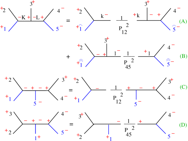
Figure 1: Factorization of the 5-point amplitude

We have thus a recursion relation, which expresses a five-point amplitude into a sum of products of three and four-point on-shell amplitudes.

Furthermore, we see that the above result is also easily obtained, if we define

$$\hat{A}(z)={1\over\hat{P}_{12}^{2}}{1\over\hat{P}_{45}^{2}},$$ (4.8)

and perform the integral

$$\oint{dz\over z}\hat{A}(z)=0$$ (4.9)

over a closed contour in the complex a-plane. The physical amplitude is $\hat{A}(z=0)$, which is the left hand side, which is one of the poles in the integral. It is also given as the sum of the residues due to the other two poles of $\hat{A}(z).$

5 Gauge Invariance

When we use the ’on-shell’ method to perform a calculation, we must be aware that the ’effective vertices’ are complexly continued lower point amplitudes. They are made on-shell, but they depend on the reference spinors $|+>,[-|.$ The final result, i. e. the physical amplitudes with real momenta, should be independent of any of such choice which is made for expediency. We also recall that fixing $N$ is a choice of gauge and therefore the independency on $N$ is tantamount to gauge invariance.

We explore this further in its infinitesimal form. Suppose we first make a choice

$$|+>,\ \ \ [-|,\ \ \ \ [-+]=1,$$ (5.1)

and then decide to make a small change

$$|+^{\prime}>=|+>,\ \ \ |-^{\prime}|=n([-|+\delta a[x|),$$ (5.2)

in which $n$ is a normalization factor and $[x|$ is at this point some spinor. However, when we normalize $[-^{\prime}+^{\prime}]=1$, we find that $[x|=[+|$ is the only solution and therefore

$$[-^{\prime}|=[-|+\delta a[+|.$$ (5.3)

The requirement of gauge invariance is that physical amplitudes with real external momenta should be independent of $\delta a$.

We learn from experience that gauge invariance imposes very stringent conditions on physical amplitudes. If there are several diagrams for a process, gauge invariance relates them in some mysterious way to cause tremendous amounts of cancellations to yield a simple result. Even though the ’on-shell’ method saves plenty of unnecessary labor, the cancellations are still incomplete.

Let us look at one example. We analyze a one loop calculation of $P_{1}^{-}P_{2}^{+}P_{3}^{+}P_{4}^{+}$, with the choice

$$|+>=|p_{1}>,\ \ \ [-|=[p_{3}|.$$ (5.4)

We would like to make a remark with regard to complexificaton by shifting momenta. In order to reveal all the poles in the kinematical invariants that we are interested in, which transcribe into poles in the $z$-plane, we must choose shifts and reference spinors properly. For this example, one set of shifts is

$$[\hat{1}|=[1|+z[24][-|,\ \ \ |\hat{1}>=|1>,$$ (5.5)

$$[\hat{2}|=[2|,\ \ \ |\hat{2}>-|2>+z[4-]||1>,$$ (5.6)

$$[\hat{3}|=[3|,\ \ \ |\hat{3}>=|3>,$$ (5.7)

$$[\hat{4}|=[4|,\ \ \ |\hat{4}>=|4>+z[-2]|1>,$$ (5.8)

which preserve overall energy momentum conservation. We find that there are three diagrams which make up this process, two of which are one particle reducible (1PR) and are easy to obtain and one is irreducible and requires some hard calculation.

Figure 2: The 4-point one-loop (+++-) amplitude

From consideration of its collinear behavior, one can show that

$$A_{4}=A^{1PR}_{4s}f_{s}+A^{1PR}_{4u}f_{u}.$$ (5.9)

When we make an infinitesimal gauge change, we have

$$0=\delta A_{4}=[(\delta A^{1PR}_{4s})f_{s}+A^{1PR}_{4s}(\delta f_{s})]+[(\delta A^{1PR}_{4u})f_{u}+A^{1PR}_{4u}(\delta f_{u})].$$ (5.10)

The pole structure in $s=-(P_{1}+P_{2})^{2}$ and $u=-(P_{1}+P_{4})^{2}$ dictates that each pair of parenthesis should vanish

$${\delta f_{s}\over f_{s}}=-{\delta A^{1PR}_{4s}\over A^{1PR}_{4s}},\ \ \ {\delta f_{u}\over f_{u}}=-{\delta A^{1PR}_{4u}\over A^{1PR}_{4u}},$$ (5.11)

The right hand sides are known and we can solve these equations to yield

$$f_{s}={-t\over u},\ \ \ f_{u}={-t\over s},\ \ \ t=-(s+u).$$ (5.12)

We have a recursion relation, which connects four-point ampitudes to three-point amplitudes. $f$’s are known as soft factors, and were postulated in Ref.[6].

This line of reasoning can be used for the evaluation of one loop amplitudes for $n$ gluons with all but one having the same helicity. Also, there are recursion relations for the one loop gluon amplitudes with all + or all - helicity. They do not need any soft factors [6, 14].

6 Concluding Remarks

There is still much to be uncovered in non-Abelian gauge theories. We have used the freedom of choice in $|+>,[-|$ and complex momentum shifts to explore the analyticity of its scattering amplitudes. The analysis is further simplified and augmented by the use of space-cone gauge. Much more can be and needs to be done.

There have been fruitful exchanges and inspiration between non-Abelian theories and higher dimensional conformal field theories and strings, particularly in calculational aspects of scattering amplitudes [2, 3, 4, 15, 16]. Through these infusions, one may even gain a better understanding of the strong coupling limit.

We have discussed those amplitudes which are rational functions of spinor products. For more complicated helicity arrangements, there is a lot of new developments, such as spinor/twistor integrations, generalized unitarity, loop integral evaluations, etc. They can only enrich the tool box.

All these are of interest to many of us, because of the relevance of non-Abelian fields to real physics, a tribute to Professor Yang’s deep insight some fifty years ago.

References

-
[1]
Z. Bern, L. J. Dixon, D. C. Dunbar and D. A. Kosower,
“Fusing gauge theory tree amplitudes into loop amplitudes,” Nucl. Phys. B 435, 59 (1995) [arXiv:hep-ph/9409265]. -
[2]
E. Witten,
“Perturbative gauge theory as a string theory in twistor space,” Commun. Math. Phys. 252, 189 (2004) [arXiv:hep-th/0312171]. -
[3]
F. Cachazo, P. Svrcek and E. Witten,
“MHV vertices and tree amplitudes in gauge theory,” JHEP 0409, 006 (2004) [arXiv:hep-th/0403047]. -
[4]
R. Britto, F. Cachazo and B. Feng,
“New recursion relations for tree amplitudes of gluons,” Nucl. Phys. B 715, 499 (2005) [arXiv:hep-th/0412308]. -
[5]
R. Britto, F. Cachazo, B. Feng and E. Witten,
“Direct proof of tree-level recursion relation in Yang-Mills theory,” Phys. Rev. Lett. 94, 181602 (2005) [arXiv:hep-th/0501052]. -
[6]
Z. Bern, L. J. Dixon and D. A. Kosower,
“On-shell recurrence relations for one-loop QCD amplitudes,” Phys. Rev. D 71, 105013 (2005) [arXiv:hep-th/0501240]. - [7] F. A. Berends, R. Kleiss, P. De Causmaecker, R. Gastmans and T. T. Wu, Phys. Lett. B103, 124 (1981). Z. Xu, D.-H. Zhang and L. Chang, Nucl. Phys. B291, 392 (1987).
- [8] S. Parke and T. Taylor, Phys. Rev. Lett. 56, 2450 (1986).
-
[9]
G. Chalmers and W. Siegel,
“Simplifying algebra in Feynman graphs. II: Spinor helicity from the spacecone,” Phys. Rev. D 59, 045013 (1999) [arXiv:hep-ph/9801220]. -
[10]
M. J. G. Veltman,
“Unitarity And Causality In A Renormalizable Field Theory With Unstable Particles,” Physica 29, 186 (1963). - [11] J. Schwinger, J. Math. Phys. 2. 407 (1961). For a more extended treatment, see e. g. K.-C. Chou, Z.-B. Su, B.-L. Hao and L. Yu, Phys. Reports 118, nos. 1 and 2, (1988).
-
[12]
R. F. Streater and A. S. Wightman,
PCT, Spin & Statics and all that, The Mathematical Physics Monograph Series, ed. W. A. Benjamin, Inc (1964). -
[13]
D. Vaman and Y. P. Yao,
“QCD recursion relations from the largest time equation,” JHEP 0604, 030 (2006) [arXiv:hep-th/0512031]. -
[14]
D. Vaman and Y. P. Yao,
“On-shell QCD recurrence relations and the space-cone gauge ,” 42d Rencontres de Moriond, La Thuile, Italy, 10-24 March 2007, QCD Electronic Proceedings: http://events.lal.in2p3.fr/Moriond/PDF_PROC_QCD/vaman%20-%20copie.pdf - [15] J. M. Maldacena, “The large N limit of superconformal field theories and supergravity,” Adv. Theor. Math. Phys. 2, 231 (1998) [Int. J. Theor. Phys. 38, 1113 (1999)] [arXiv:hep-th/9711200].
- [16] L. F. Alday and J. M. Maldacena, “Gluon scattering amplitudes at strong coupling,” JHEP 0706, 064 (2007) [arXiv:0705.0303 [hep-th]].