Journal of Physics B: At. Mol. Opt. Phys. 41 (2008) 235503

We explore and develop the mathematics of the two multi-level ions. In particular, we describe some new features of quantum entanglement in two three-level trapped ions confined in a one-dimensional harmonic potential, allowing the instantaneous position of the center-of-mass motion of the ions to be explicitly time-dependent. By solving the exact dynamics of the system, we show how survivability of the quantum entanglement is determined by a specific choice of the initial state settings.

1 Introduction

The ability to laser cool ions within the vicinity of the motional ground state is a key factor in the realization of efficient quantum communication [1]. Laser-cooled ions confined in an electromagnetic trap are good candidates for various quantum information processing processes such as quantum control and quantum computing [2]. Various interactions models and higher order non-linear models can be implemented in this system by simply choosing appropriate applied laser tunings [3, 4]. For more than one ion, as required in any realistic quantum logic schemes, individual addressing imposes small trap frequencies, whereas sideband cooling imposes high trap frequencies [5]. Experimentally, the sideband cooling of two ions to the ground state has been achieved in a Paul trap that operates in the Lamb-Dicke limit [6]. Recent advances in the dynamics of trapped ions [7]) have demonstrated that a macroscopic observer can effectively control dynamics as well as perform a complete measurement of states of microscopic quantum systems.

On the other hand, entanglement is the quintessential property of quantum mechanics that sets it apart from any classical physical theory, and it is essential to quantify it in order to assess the performance of applications of quantum information processing [8]. With the reliance in the processing of quantum information on a cold trapped ion, a long-living entanglement in the ion-field interaction with pair cat states has been observed [9]. Also, experimental preparation and measurement of the motional state of a trapped ion, which has been initially laser cooled to the zero-point of motion, has been reported in [10]. It is well known that the loss of entanglement cannot be restored by local operations and classical communications, which is one of the main obstacles to build up a quantum computer [11]. Therefore it becomes an important subject to study entanglement dynamics of qubits [12, 13, 14, 15, 16, 17]. Quite recently, it has been shown that entanglement of two-qubit systems can be terminated abruptly in a finite time in the presence of either quantum or classical noises [12, 17]. This non-smooth finite-time decay has been referred as entanglement sudden death (ESD) [12, 18, 19]. At least two experimental verifications of ESD have been reported so far [20, 21]. Interestingly, as the entanglement can suddenly disappear, it can be suddenly generated, a process called entanglement sudden birth [22].

These recent results together with the fundamental interest of the subject, are the motivation for the present work: we study here the entanglement evolution of two three-level trapped ions interacting with a laser field taking into account the time-dependent modulated function. We focus our attention on the entanglement decay and generation due to the presence of a time-dependent modulated function in the two interacting ions and intrinsic decoherence. We show that entanglement of two ions in the Lamb-Dicke regime presents some novel features with respect to single-trapped ion. In particular, we show how sudden feature in the entanglement(sudden birth and sudden death of entanglement) occurs for the two-ion system coupled to a laser field.

The paper is organized as follows. In section 2, we introduce the model and define the different parameters which will be used throughout the paper. We devote section 3 to an alternative approach to find an exact dynamics of the coupled system in the presence of the time-dependent modulated function. Section 4 is devoted to study some examples of entanglement evolutions which lead to different types of decay for entangled systems, and show how different initial state settings and time-dependent interaction affect the decay of the entanglement. Then we conclude the paper with some remarks on how the presented results could be generalized to multi-ions systems.

2 Model

A useful model of controlled entanglement evolution consists of two three-level ions that are irradiated by laser beams whose wavevectors lie in the radial plane of the trap. This laser configuration excites the vibrational motion in the radial plane only ($1D$ ionic motion) [23, 24]. Therefore, the physical system on which we focus is two three-level harmonically trapped ions with their center-of-mass motion quantized. We denote by $a$ and $a^{\dagger}$ the annihilation and creation operators and $\upsilon$ is the vibrational frequency related to the center-of-mass harmonic motion along the direction $\hat{x}.$ Without the rotating wave approximation, the trapped ions Hamiltonian for the system of interest may be written as

$$\hat{H}=\hat{H}_{cm}+\hat{H}_{ion}+\hat{H}_{int},$$ (1)

where

$$\hat{H}_{cm} = \hbar\upsilon\hat{a}^{\dagger}\hat{a},\qquad$$

$$\hat{H}_{ion} = \sum\limits_{i=1}^{2}\sum\limits_{j=a,b,c}\hbar\omega_{i}S_{jj}^{(i)},$$

$$\hat{H}_{int}(t) = \hbar\Im(\hat{x},t)\hat{S}_{ab}^{(1)}+\hbar\Im^{\ast}(\hat{x},t)\hat{S}_{ba}^{(1)}+\hbar\Im(\hat{x},t)\hat{S}_{ab}^{(2)}+\hbar\Im^{\ast}(\hat{x},t)\hat{S}_{ba}^{(2)}$$ (2)

$$+\hbar\Im(\hat{x},t)\hat{S}_{ac}^{(1)}+\hbar\Im^{\ast}(\hat{x},t)\hat{S}_{ca}^{(1)}+\hbar\Im(\hat{x},t)\hat{S}_{ac}^{(2)}+\hbar\Im^{\ast}(\hat{x},t)\hat{S}_{ca}^{(2)}.$$

We denote by $\hat{S}_{lm}^{(i)}$ the atomic flip operator for the $|m\rangle_{i}\rightarrow|l\rangle_{i}$ transition between the two electronic states, where $\hat{S}_{lm}^{(i)}=|l\rangle_{ii}\langle m|,(l,m=a,b,c)$. Suppose the ions are irradiated by a laser field of the form $\Im(\widehat{r},t)=\hbar^{-1}\epsilon\langle i|d.\wp|j\rangle\exp[-i(k\widehat{r}-\Omega t)],$ where $\epsilon$ is the amplitude of the laser field with frequency $\Omega$ and polarization vector $\wp$. The transition in the three-level ions is characterized by the dipole moment $d$ and $k$ is the wave vector of the laser field. Therefore if we express the center of mass position in terms of the creation and annihilation operators of the one-dimensional trap namely $\hat{x}=\Delta x(a^{\dagger}+a),$ where $\Delta x=(\hbar/2\upsilon m)^{1/2}=\eta/k$ is the widths of the dimensional potential ground states, in the $x$ direction ($\eta$ is called Lamb–Dicke parameter describing the localization of the spatial extension of the center-of-mass), and $m$ is the mass of the ions.

By using a special form of Baker-Hausdorff theorem [3], the operator $\exp[i\eta(a^{\dagger}+a)]$ may be written as a product of operators i.e. $\exp(i\eta(a^{\dagger}+a))=\exp\left(\frac{\eta^{2}}{2}[a^{\dagger},a]\right)\exp\left(i\eta a^{\dagger}\right)\exp\left(i\eta a\right).$ The physical processes implied by the various terms of the operator

$$\exp\left(i\eta\left(a^{\dagger}+a\right)\right)=\exp\left(\frac{-\eta^{2}}{2}\right)\sum_{n=0}^{\infty}\frac{\left(i\eta\right)^{n}a^{\dagger n}}{n!}\sum_{m=0}^{\infty}\frac{\left(i\eta\right)^{m}a^{m}}{m!},$$ (3)

may be divided into three categories (i) the terms for $n>m$ correspond to an increase in energy linked with the motional state of center of mass of the ion by ($n-m$) quanta, (ii) the terms with $n<m$ represent destruction of ($m-n$) quanta of energy thus reducing the amount of energy linked with the center of mass motion and (iii) ($n=m$), represents the diagonal contributions. When we take Lamb-Dicke limit and apply the rotating wave approximation discarding the rapidly oscillating terms, the interaction Hamiltonian (2) takes a simple form

$$\hat{H}_{int} = \sum\limits_{i=1}^{2}\left(\hbar\lambda_{1}^{(i)}(t)\mathcal{E}(a^{\dagger}a)\hat{S}_{12}^{(i)}a^{\dagger}+\hbar\lambda_{1}^{(i)\ast}(t)\mathcal{E}^{\ast}(a^{\dagger}a)\hat{S}_{21}^{(i)}a\right)$$ (4)

$$+\left(\hbar\lambda_{2}^{(i)}(t)\mathcal{E}(a^{\dagger}a)\hat{S}_{13}^{(i)}a^{\dagger}+\hbar\lambda_{2}^{(i)\ast}(t)\mathcal{E}^{\ast}(a^{\dagger}a)\hat{S}_{31}^{(i)}a\right),$$

where $\lambda_{j}^{(i)}(t)$ is a new coupling parameter adjusted to be time dependent. The other contributions which rapidly oscillate with frequency $\nu$ have been disregarded. Note that in the Lamb-Dicke regime only processes with first and second order of $\eta$ are considered, while in the general case, the nonlinear coupling function is derived by expanding the operator-valued mode function as

$$\mathcal{E}_{k}(a^{\dagger}a)=-\frac{\epsilon}{2}\exp\left(-\frac{\eta^{2}}{2}\right)\sum\limits_{n=0}^{\infty}\frac{(i\eta)^{2n+k}}{n!(n+k)!}a^{\dagger n}a^{n}.$$ (5)

Since $\mathcal{E}_{k}(a^{\dagger}a)$ depends only on the quantum number $a^{\dagger}a$, in the basis of its eigenstates, $a^{\dagger}a|n\rangle=n|n\rangle$, ($n=0,1,2,...$), these operators are diagonal, with their diagonal elements $\langle n|\mathcal{E}_{k}(a^{\dagger}a)|n\rangle$ is given by $\mathcal{E}_{k}^{(j)}(n)=-0.5\epsilon(n+k)!)^{-1}n!L_{n}^{k}(\eta^{2})\exp\left(-\eta^{2}/2\right)$ where $L_{n}^{k}(\eta^{2})$ are the associated Laguerre polynomials.

3 Solution

3.1 Master equation

To study the time evolution of the quantum entanglement, we will start by finding the general solution of the two-ion system with the Hamiltonian ( 4).  The intrinsic decoherence approach [25], is based on the assumption that on sufficiently short time scales the system does not evolve continuously under unitary evolution but rather in a stochastic sequence of identical unitary transformations. Under the Markov approximation [25], the master equation governing the time evolution for the two-ion system under the intrinsic decoherence is given by

$$\frac{d}{dt}\hat{\rho}(t)=-\frac{i}{\hbar}[\hat{H},\hat{\rho}]-\frac{\gamma}{2\hbar^{2}}[\hat{H},[\hat{H},\hat{\rho}]],$$ (6)

where $\gamma$ is the intrinsic decoherence parameter. The first term on the right-hand side of equation (6) generates a coherent unitary evolution of the density matrix, while the second term represents the decoherence effect on the system and generates an incoherent dynamics of the coupled system. In order to obtain an exact solution for the density operator $\hat{\rho}(t)$ of the master equation (6), three auxiliary superoperators $\widehat{J},\widehat{S}$ and $\widehat{L}$ can be introduced as ($\hbar=1)$

$$\exp\left(\widehat{J}\tau\right)\hat{\rho}(t) = \sum\limits_{k=0}^{\infty}\frac{\left(\gamma\tau\right)^{k}}{k!}\hat{H}^{k}\hat{\rho}(t)\hat{H}^{k},$$

$$\exp\left(\widehat{S}\tau\right)\hat{\rho}(t) = \exp\left(-i\hat{H}\tau\right)\hat{\rho}(t)\exp\left(i\hat{H}\tau\right),$$ (7)

$$\exp\left(\widehat{L}\tau\right)\hat{\rho}(t) = \exp\left(-\frac{\tau\gamma}{2}\hat{H}^{2}\right)\hat{\rho}(t)\exp\left(-\frac{\tau\gamma}{2}\hat{H}^{2}\right),$$

where $\widehat{J}\hat{\rho}(t)=\gamma\hat{H}\hat{\rho}(t)\hat{H},$ $\widehat{S}\hat{\rho}(t)=-i[\hat{H},\hat{\rho}(t)]$ and $\widehat{L}\hat{\rho}(t)=-(\gamma/2)(\hat{H}^{2}\hat{\rho}(t)+\hat{\rho}(t)\hat{H}^{2}).$ Then, it is straightforward to write down the formal solution of the master equation (6) as follows

$$\hat{\rho}(t) = \exp(\widehat{J}t)\exp(\widehat{S}t)\exp(\widehat{L}t)\hat{\rho}(0)$$ (8)

$$= \sum_{k=0}^{\infty}\hat{M}_{k}(t)\hat{\rho}(0)\hat{M}_{k}^{\dagger}(t).$$

We denote by $\hat{\rho}(0)$ the density operator of the initial state of the system and $\hat{M}_{k}=\frac{\left(\gamma t\right)^{k/2}}{\sqrt{k!}}\hat{H}^{k}\exp\left(-i\hat{H}t\right)\exp\left(-\frac{\gamma t}{2}\hat{H}^{2}\right)$, where the so-called Kraus operators $\hat{M}_{k}$ satisfy $\sum\limits_{k=0}^{\infty}\hat{M}_{k}(t)\hat{M}_{k}^{\dagger}(t)=\hat{I}$ for all $t$.

Eq. (8) can also be written as

$$\hat{\rho}(t)=e^{-i\hat{H}t}\exp\left(-\frac{\gamma t}{2}\hat{H}^{2}\right)\left\{e^{\left(\hat{S}_{M}t\right)}\hat{\rho}(0)\right\}\exp\left(-\frac{\gamma t}{2}\hat{H}^{2}\right)e^{i\hat{H}t},$$ (9)

where, we define the superoperator $\hat{S}_{M}\hat{\rho}(0)=\gamma\hat{H}\hat{\rho}(0)\hat{H}$. The reduced density matrix of the ions is given by taking the partial trace over the field system, i.e. $\rho^{a}(t)\equiv tr_{F}\rho(t)=\rho_{ij,lk}(t)|ij\rangle\langle lk|.$ We use the notation $|ij\rangle=|i_{1}\rangle\otimes|j_{2}\rangle,$ $(i,j=a,b,c),$ where $|a_{1(2)}\rangle,$ $|b_{1(2)}\rangle$ and $|c_{1(2)}\rangle$ are the basis states of the first (second) ion and $\rho_{ij,lk}(t)=\langle ij|\rho^{a}(t)|lk\rangle$ corresponds the diagonal ($ij=lk$) and off-diagonal ($ij\neq lk)$ elements of the density matrix $\rho^{a}(t).$

It is worth referring here to the fact that, Eq. (9) represents the general solution of the master equation (6) that can be used to study the effect of the intrinsic decoherence when the modulated function $\lambda_{j}^{(i)}(t)$ is taken to be time-independent. However, to study the time-dependent case as seen below, it will be much more convenient to use the exact wave function.

3.2 Wave function

At any time the state vector $\left|\Psi(t)\right\rangle$ in the interaction picture can be written as

$$\left|\Psi(t)\right\rangle=\sum\limits_{i=1}^{9}\sum\limits_{n=0}^{\infty}A_{i}(n,t)\left|\psi_{i}\right\rangle.$$ (10)

where $\left|\psi_{1}\right\rangle=\left|n;a_{1}a_{2}\right\rangle,\left|\psi_{2}\right\rangle=\left|n+1;a_{1}b_{2}\right\rangle,$ $\left|\psi_{3}\right\rangle=\left|n+1;a_{1}c_{2}\right\rangle,$ $\left|\psi_{4}\right\rangle=\left|n+1;b_{1}a_{2}\right\rangle,\left|\psi_{5}\right\rangle=\left|n+2;b_{1}b_{2}\right\rangle,$ $\left|\psi_{6}\right\rangle=\left|n+2;b_{1}c_{2}\right\rangle,$ $\left|\psi_{7}\right\rangle=\left|n+1;c_{1}a_{2}\right\rangle,$ $\left|\psi_{8}\right\rangle=\left|n+2;c_{1}b_{2}\right\rangle,$ $\left|\psi_{9}\right\rangle=\left|n+2;c_{1}c_{2}\right\rangle,$ where $\left|n\right\rangle$ corresponds to the initial state of the vibrational motion. We denote by $A_{i}(n,t)$ the probability amplitude for the ion to be in the state $\left|\psi_{i}\right\rangle$. In general, the dynamics of the probability amplitudes $A_{i}(n,t)$ is given by the Schrödinger equation,

$$i\frac{\partial A_{j}(n,t)}{\partial t}=\sum\limits_{l=1}^{9}C_{jl}A_{l}(n,t),$$ (11)

where $C_{jk}=\left\langle\psi_{j}\right|\hat{H}_{int}\left|\psi_{k}\right\rangle.$ These equations are exact for any two three-level system. In order to consider the most general case, we solve equation (11), by assuming a new variable $G(n,t)$ as $G(n,t)=\sum\limits_{i=1}^{9}x_{i}A_{i}(n,t),$where $x_{1}=1,$ which means that

$$i\frac{dG(n,t)}{dt}=\gamma(t)\beta_{1}\left(A_{1}(n,t)+\sum\limits_{i=2}^{9}\beta_{i}^{\prime}A_{i}(n,t)\right),$$ (12)

where $\lambda_{j}^{(i)}(t)=\gamma(t)\lambda_{j}$ and $\beta_{i}$ are given by $\beta_{1}=x_{2}C_{21}+x_{3}C_{31}+x_{4}C_{41}+x_{7}C_{71},$ and $\beta_{i}^{\prime}=\beta_{i}/\beta_{1},$ where $\beta_{2}=C_{11}+x_{5}C_{51}+x_{8}C_{81},$ $\beta_{3}=C_{13}+x_{6}C_{63}+x_{9}C_{93},$ $\beta_{4}=C_{14}+x_{5}C_{54}+x_{6}C_{64},$ $\beta_{5}=x_{2}C_{25}+x_{4}C_{45},$ $\beta_{6}=x_{3}C_{36}+x_{4}C_{46},$ $\beta_{7}=C_{17}+x_{8}C_{87}+x_{9}C_{97},$ $\beta_{8}=x_{2}C_{28},$ $\beta_{9}=x_{3}C_{39}+x_{7}C_{79},$

Let us emphasize that in addition to the general form of equation (12 ), the present method is also suitable for any initial conditions. It is instructive to examine the formation of a general solution of the two three-level systems. Therefore, we use equation (12) and seek $G(n,t)$ such that $i\dot{G}(n,t)=z\zeta(t)G(n,t).$ This holds if $\beta_{1}=z$ and $\beta_{i}=x_{i}.$ Some simple algebra gives rise to an equation that has nine eigenvalues such that the $z_{i}$ [26] are determined. Correspondingly, there are also nine corresponding eigenfunctions

$$G_{j}(n,t)=G_{j}(0)\exp\left(-iz_{j}\int_{0}^{t}\zeta(\tau)d\tau\right),$$ (13)

where $G_{j}(n,t)=\sum\limits_{k=1}^{9}M_{jk}A_{k}(n,t),$ and $M_{ji}=\widehat{p}^{T}\hat{e}_{xi}+\sum\limits_{i=1}^{9}\hat{x}_{i}^{T}\hat{e}_{xi}.$ We denote by $\hat{e}_{xi}$ mutually orthogonal unit vectors, given by $\hat{e}_{x_{i}}=(\delta_{i1},\delta_{i2},\delta_{i3},\delta_{i4},\delta_{i5},\delta_{i6},\delta_{i7},\delta_{i8},\delta_{i9}),$ $\delta_{ij}=1$ if $i=j$ and $\delta_{ij}=0$ if $i\neq j$ and $\widehat{p}=(1,1,1,1,1,1,1,1,1),$ $\hat{x}_{i}=(x_{i1},x_{i2},x_{i3},x_{i4},$ $x_{i5},x_{i6},$ $x_{i7},$ $x_{i8},x_{i9}).$ Then, one can express the unperturbed state amplitude $A_{i}(n,t)$ in terms of the dressed state amplitude $G_{j}(n,t)$ as follows

$$A_{i}(n,t)=\sum\limits_{j=1}^{9}M_{ij}^{-1}G_{j}(n,t)=\sum\limits_{j=1}^{9}M_{ij}^{-1}G_{j}(0)\exp\left(-iz_{j}\int_{0}^{t}\zeta(\tau)d\tau\right).$$ (14)

We have thus completely determined the exact solution of a two three-level system in the presence of the time-dependent modulated function.

4 Entanglement evolution

Good measures of entanglement are invariant under local unitary operations. They are also required to be entanglement monotones, that is, they must be non-increasing under local quantum operations combined with classical communication [27, 28, 29, 30, 31, 32]. computable entanglement measures for a generic multiple level system do not exist. For two-qubit systems, concurrence can be used to compute entanglement for both pure and mixed states [33]. Rungta et al [34] defined the so-called I-concurrence in terms of a universal-inverter which is a generalization to higher dimensions of two spin flip operation, therefore, the concurrence in arbitrary dimensions takes the form

$$I_{\psi}\left(t\right)=\sqrt{\langle\psi|S_{N_{1}}\otimes S_{N_{1}}(|\psi\rangle\langle\psi|)|\psi\rangle}.$$ (15)

Another generalization is proposed by Audenaert et al [35] by defining a concurrence vector in terms of a specific set of antilinear operators. As a complete characterization of entanglement of a bipartite state in arbitrary dimensions may require a quantity which, even for pure states, does not reduce to single number [36], Fan et al. defined the concept of a concurrence hierarchy as $N-1$ invariants of a group of local unitary for $N-$level systems [37].

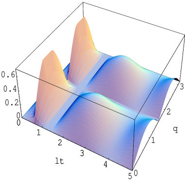
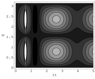
Figure 1: The evolution of the concurrence $I_{\psi}\left(t\right)$ as a function of the scaled time $\lambda_{1}t$ and $\theta.$ The parameters are $\overline{n}=5,$ $\lambda_{2}/\lambda_{1}=0.01$, and $\varphi=0.$

Now, we suppose that the initial state of the principle system is given by

$$|\psi(0)\rangle=\left(\cos\theta|a_{1},b_{2}\rangle+\sin\theta e^{i\phi}|b_{1},a_{2}\rangle\right)\otimes\sum\limits_{n=0}^{\infty}q_{n}|n\rangle,$$ (16)

where $\theta\in[0,2\pi],$ $\phi\in[0,\pi]$ and $q_{n}=\langle n|\psi(0)\rangle.$

In absence of intrinsic decoherence, the concurrence (15) will be calculated using Eq. (10), while to study the effect of $\gamma$ we use equation (9). In figures 1 and 2 the dependence on $\theta$ and the scaled time $\lambda_{1}t,$ in the Lamb-Dicke regime, of the concurrence $I_{\psi}\left(t\right)$ is illustrated. In the typical experiments at NIST [39], ${}^{9}Be^{+}$ ions are stored in a RF Paul trap with a secular frequency along $\widehat{x}$ of $\nu/2\pi\simeq 11.2$ MHz, providing a spread of the ground state wave function of $\Delta x\simeq 7$ nm, with a Lamb-Dicke parameter of $\eta\simeq 0.202$. With these data we find $\epsilon\simeq 0.01$, so they can be considered as small parameters. We see that the concurrence $I_{\psi}\left(t\right)$ exhibits some peaks whose amplitude decreases as the interaction time increases. The main consequence is that we can select a given value of the superposition parameter $\theta$, or rather a specific instant time to obtain strong entanglement or disentanglement.

The entanglement sudden birth phenomenon is observed in figure 1. Entanglement is not present at earlier times, and suddenly at some finite time an entanglement starts to build up. Also, from figure 1, it is clearly seen that the value of first local maximum significantly exceeds the second local maximum when the two ions start from a superposition state. Recall that the entanglement attains the zero value (i.e., disentanglement) when the trapped ions start from either $|a_{1},b_{2}\rangle$ or $|b_{1},a_{2}\rangle$ states, while strong entanglement occurs when the inversion is equal to zero, i.e, the two ions start from a maximum entangled state, such as $|\psi_{AB}(0)\rangle=\left(|a_{1},b_{2}\rangle+|b_{1},a_{2}\rangle\right)/\sqrt{2}$. In other words, for the initial entangled state, there are some intervals of the interaction time where the entanglement reaches its local maximum and drops to zero (entanglement sudden death).

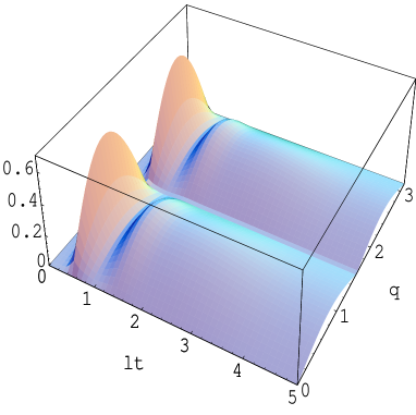
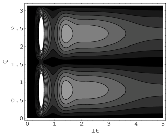
Figure 2: The same as figure 1 but $\overline{n}=15.$

To gain more insight into the general behavior of the quantum entanglement evolution, we plot in figure 2 the time evolution of the generalized concurrence $I_{\psi}\left(t\right)$ for a larger value of the field intensity, $\overline{n}$. It can be seen that the dynamics is strongly modified where a smooth decay of the entanglement is observed. In contrast to the dynamics with the small $\overline{n}$, where the sudden death of entanglement-like feature has been observed after the first local maximum of the entanglement (see figures 1 and 2), here the entanglement smoothly decays and vanishes as the time increased further. Note that the effect of the superposition parameter $\theta$ on the entanglement distributions in both figure 1 and 2 is similar and shows symmetry around $\theta=\frac{\pi}{2}$ while the local maxima correspond to $\theta=\frac{n\pi}{4},(n=1,3,5,...)$. Obviously from these figures, if $\theta=\frac{n\pi}{2},(n=0,1,2,...)$ i.e., the system starts from a separable state, the entanglement is always zero. On the other hand, if the system starts from an entangled state and because of the existence of further system parameters, the entanglement decay occurs with small or large values of $\overline{n}$. Moreover, comparison of figures 1-2 shows that the entanglement decay takes a longer time to reach zero in the case where large $\overline{n}$ is considered. We hence come to understand that considering a large intensity of the initial state of the field, can be used positively in preventing entanglement sudden death or delaying the disentanglement of the two ions. A physical explanation of why is the intensity of the field playing such a role in the disentangling process of the two ions, is that the strong field providing some sort of shielding mechanism to the decoherence effectively induced by the trace over the motional degree of freedom.

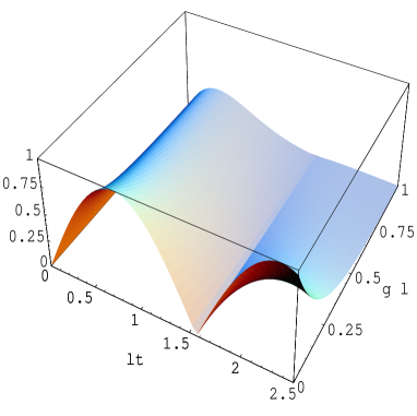
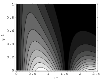
Figure 3: The concurrence as a function of the scaled time and decoherence parameter. The other parameters are the same as figure 1.

Quantum coherence and entanglement typically decay as the result of the influence of decoherence and much effort has been directed to extend the coherence time of systems of interest. However, it has been shown that under particular circumstances where there is even only a partial loss of coherence of each ion, entanglement can be suddenly and completely lost [12]. This has motivated us to consider the question of how decoherence effects the scale of entanglement in the system under consideration. Once the decoherence taken into account, i.e., $\gamma\neq 0$, it is very clear that the decoherence plays a usual role in destroying the entanglement. In this case and for different values of the decoherence parameter $\gamma,$ we can see from figure (3) that after switching on the interaction the entanglement function increases to reach its maximum showing strong entanglement. However its value decreases after a short period of the interaction time to reach its minimum. The function starts to increase its value again however with lower local maximum values showing a strong decay as time goes on. Also, from numerical results we note that with the increase of the parameter $\gamma$, a rapid decay of the entanglement (entanglement sudden death) is shown [15, 38].

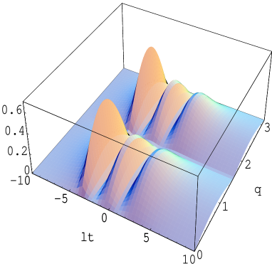
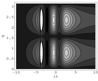
Figure 4: The same as figure 1 but the modulated function $\zeta(t)=\sec$h$\left(t/2\tau\right).$

The above results and connections are very intriguing, and naturally lead us to ask what is the role played by the modulated function in obtaining these associated phenomena of the entanglement. In order to answer this question, we consider the modulated function $\zeta(t)$ to be time-dependent of the form $\zeta(t)=\sec$h$\left(t/2\tau\right)$ [40, 41]. In this form the coupling increases from a very small value at large negative times to a peak at time $t=0$, to decrease exponentially at large times. Thus, depending on the value of $\tau$ and the initial time $t_{0}$, various limits such as adiabatically or rapidly increasing (for $t_{0}<\lambda t\leq 0$) or decreasing (for $0\leq\lambda t<t_{0}$) coupling can be conveniently studied. This allows us to investigate, analytically, the effect of transients in various different limits of the effect of switching the interaction on and off in the ion-field system. The vanishing of the interaction at large positive times leads to the leveling out of the inversion.

It should be noted that the time dependence specified in $\zeta(t)$ is one of a class of generalized interactions that may offer analytical solutions. It is evident from figure 4 that the entanglement sudden birth phenomenon is more clearly observed for the time-dependent interaction. In this case, the entanglement starts suddenly to build up at later times compared with the time-independent case. At this point the entanglement from zero evolves to its local maximum value and then oscillates with lower local maximum followed by smooth decay (see figure 4). Although increasing the field intensity leads to strong entanglement (maximum value of entanglement), however the local maximum values of the entanglement also vary and occur for some short periods of the interaction time. This indicates that in a regime where coherent state is considered, the underlying states are highly entangled. Consequently, the presence of the time-dependent modulated function increases the number of oscillations and delays the disentanglement. All these results confirm the possibility of a practical observation of time-dependence of the modulated function effects for prolonging time for the disentanglement. Our results here show the important role played by the modulated function in the entanglement dynamics which is crucial for the onset of either entanglement sudden death or sudden birth in the trapped ion systems considered in this paper. In addition, our results suggest that the analytical results presented here, could be attained for different configurations of any two trapped ions systems [42].

The remaining task is to identify and compare the results presented above for the entanglement with another accepted entanglement measure such as the quantum relative entropy. Eisert and Plenio [43] have raised the question of the ordering of entanglement measures. It has been proven that all good asymptotic entanglement measures are either identical or fail to uniformly give consistent orderings of density matrices [44]. One of the best understood cases is entanglement measure defined in terms of the quantum relative entropy. More explicitly, for the entangled states $\hat{\rho}(t)$ the quantum relative entropy is defined by the following formula as the distance between the entangled state $\hat{\rho}(t)$ and disentangled state $tr_{\mathcal{A}}\hat{\rho}(t)\otimes tr_{\mathcal{B}}\hat{\rho}(t)\in\mathfrak{S}(\mathcal{H}_{1}\otimes\mathcal{H}_{2})$ [45, 46]

$$I_{\rho}\left(\rho_{t}^{\mathcal{A}},\rho_{t}^{\mathcal{B}}\right)=tr\hat{\rho}(t)(\log\hat{\rho}(t)-\log(tr_{\mathcal{A}}\hat{\rho}(t)\otimes tr_{{}_{\mathcal{B}}}\hat{\rho}(t))),$$ (17)

where $\rho_{t}^{\mathcal{A}}=tr_{\mathcal{B}}\left(\hat{\rho}(t)\right)$ and $\rho_{t}^{\mathcal{B}}=tr_{\mathcal{A}}\left(\hat{\rho}(t)\right),$ $\mathcal{A(B)}$ refers to the first (second) ion. Note that if the entangled state $\hat{\rho}(t)$ is a pure state, $S(\hat{\rho}(t))=0$ and then $S(tr_{\mathcal{A}}\hat{\rho}(t))=S(tr_{\mathcal{B}}\hat{\rho}(t)),$ which means that we have $I_{\rho}\left(\rho_{t}^{A},\rho_{t}^{B}\right)=2S(tr_{\mathcal{B}}\hat{\rho}(t))$. One, possibly not very surprising, principal observation is that the numerical calculations corresponding to the same parameters, give nearly the same behavior with different scales. This means that the entanglement measured by either quantum relative entropy or concurrence measures gives rise to qualitatively the same results. We must stress, however, that no single measure alone is enough to quantify the entanglement in a multilevel system.

5 Conclusions

In summary, we have derived an intuitive extension of the standard quantum model of two three-level trapped ions interacting with a laser field to include the time-dependent modulated function and intrinsic decoherence. This study reveals that the time-dependent modulated function can be used for generating either entanglement sudden death or sudden birth depending on a proper manipulation of the initial state setting. We note that the existence of entanglement sudden death reveals a fact that the non-interacting and non-communicating two ions can abruptly lose their entanglement. Also, it will be very interesting to extend these results to the case of mixed states in the presence of the decoherence. We hope the presented results can be useful for the ongoing theoretical and experimental efforts in multi-levels particles interaction.

Acknowledgment

T. Y. acknowledges grant support from US National Science Foundation (PHY-0758016). We are grateful to Prof. A.-S. F. Obada for helpful discussions.

References

References

- [1] D. J. Wineland, C. Monroe, W. M. Itano, D. Leibfried, B. E. King, and D. M. Meekhof, J. Res. Natl. Stand. Tech. 103, 259 (1998).
- [2] J. I. Cirac and P. Zoller, Phys. Rev. Lett. 74, 4091 (1995).
- [3] C.A. Blockley, D.F. Walls and H. Kisken, Europhys. Lett. 17, 509 (1992).
- [4] W. Vogel and R.L.de Matos Filho, Phys. Rev. A 52, 4214 (1995); W. Vogel and D.-G. Welsch, ibid. 40, 7113 (1989); A. Steane, C.F. Roos, D. Stevens, A. Mundt, D. Leibfried, F. Schmidt-Kaler, and R. Blatt, ibid. 62, 042305 (2000); L.F. Wei, Y.-X. Liu, and F. Nori, Phys. Rev. A 70, 063801 (2004)
- [5] G. Morigi, J. Eschner, J. I. Cirac, and P. Zoller, Phys. Rev. A 59, 3797 (1999)
- [6] B. E. King, C. S. Wood, C. J. Myatt, Q. A. Turchette, D. Leibfried, W. M. Itano, C. Monroe, and D. J. Wineland, Phys. Rev. Lett. 81, 1525 (1998).
- [7] D. Leibfried, R. Blatt, C. Monroe and D. Wineland, Rev. Mod. Phys. 75, 281 (2003).
- [8] S. Hill and W. K. Wootters, Phys. Rev. Lett. 78, 5022 (1997); M. A. Nielsen, Phys. Rev. Lett. 83, 436 (1999).
- [9] M. Abdel-Aty, Appl. Phys. B: Laser and Opt. 84, 471 (2006).
- [10] D. Leibfried, D. M. Meekhof, B.E. King, C. Monroe, W.M. Itano and D.J. Wineland, J. Mod. Opt. 44, 2485 (1997).
- [11] C. H. Bennett, H. J. Bernstein, S. Popescu and B. Schumacher, Phys. Rev. A 53, 2046 (1996).
- [12] T. Yu and J. H. Eberly, Opt. Commun. 264, 393 (2006).
- [13] M. Yonac, T. Yu and J. H. Eberly, J. Phys. B: At. Mol. Opt. Phys. 39, S621(2006).
- [14] C. Pineda and T. H. Seligman, Phys. Rev. A 73, 012305 (2006).
- [15] T. Yu and J. H. Eberly, Phys. Rev. B 66, 193306 (2002).
- [16] T. Yu and J. H. Eberly, Phys. Rev. B 68, 165322 (2003).
- [17] T. Yu and J. H. Eberly, Phys. Rev. Lett. 93, 140404 (2004).
- [18] T. Yu and J. H. Eberly, Phys. Rev. Lett. 97, 140403 (2006).
- [19] T. Yu and J.H. Eberly, Quant. Inf. Comp. 7, 459 (2007).
- [20] M.P. Almeida et al, Science 316, 579 (2007). See also J.H. Eberly and T. Yu, Science 316, 555 (2007).
- [21] J. Laurat et al., Phys. Rev. Lett. 99, 180504 (2007).
- [22] Z. Ficek and R. Tanas, Phys. Rev. A 77, 054301 (2006); C. E. Lopez, G. Romero, F. Lastra, E. Solano and J. C. Retamal, Phys. Rev. Lett. 101, 080503 (2008).
- [23] A. Messina, S. Maniscalco and A. Napoli, J. Mod. Opt. 50, 1 (2003), M. Abdel-Aty, Prog. Quant. Electron., 31, 1 ( 2007).
- [24] S. S. Sharma and N. K. Sharma, J. Phys. B 35, 1643 (2002).
- [25] G.J. Milburn, Phys. Rev. A 44, 5401 (1991); S. Schneider and G.J. Milburn, Phys. Rev. A 57, 3748 (1998); S. Schneider and G.J. Milburn, Phys. Rev. A 59, 3766 (1999).
- [26] J. H. Mc-Guire, K. K. Shakov and K. Y. Rakhimov, J. Phys. B 36, 3145 (2003).
- [27] V. Vedral, M. B. Plenio and P. L. Knight, ”The Physics of Quantum Information”, edited by D Bouwmeester, A Ekert and A Zeilinger, Springer (2000); V. Vedral, M. B. Plenio, K. Jacobs, and P. L. Knight, Phys. Rev. A 56, 4452 (1997); G. Vidal, J. Mod. Opt. 47, 355 (2000).
- [28] S. J. D. Phoenix and P. L. Knight, Ann. Phys. (N. Y) 186, 381 (1988).
- [29] S. J. D. Phoenix and P. L. Knight, Phys. Rev. A 44, 6023 (1991).
- [30] S. J. D. Phoenix and P. L. Knight, Phys. Rev. Lett. 66, 2833 (1991).
- [31] D. W. Berry and B. C. Sanders, J. Phys. A 36, 12255 (2003).
- [32] S. Bose, I. Fuentes-Guridi, P. L. Knight, and V. Vedral, Phys. Rev. Lett. 87, 050401 (2001); S. Scheel, J. Eisert, P. L. Knight, M. and B. Plenio, J. Mod. Opt. 50, 881 (2003); E. Ciancio and P. Zanardi, Phys. Lett. A 360, 49 (2006).
- [33] W. K. Wootters, Phys. Rev. Lett. 80, 2245 (1998).
- [34] P. Rungta, V. Buzek, C. M. Caves, M. Hillery and G. J. Milburn, Phys. Rev. A 64, 042315 (2001); S. J. Akhtarshenas, J. Phys. A: Math. Gen. 38, 6777 (2005).
- [35] K. Audenaert, F. Verstraete and De Moor, Phys. Rev. A 64, 052304 (2001).
- [36] D. Meyer and N. Wallach, in The Mathematics of Quantum Computation, edited by R. K. Brylinski and G. Chen (CRC Press, Boca Raton, 2002), p. 77.
- [37] H. Fan, K. Matsumoto and H. Imati, J. Phys. A: Math. Gen. 36, 4151 (2003).
- [38] A.-S. F. Obada, and M. Abdel-Aty, Phys. Rev. B 75, 195310 (2007); M. Abdel-Aty, and H. Moya-Cessa, Phys. Lett. A 369, 372 (2007).
- [39] D. Leibfried, D. M. Meekhof, B. E. King, C. Monroe, W. M. Itano and D. J. Winel, Phys. Rev. Lett. 77, 4281 (1996); Q. A. Turchette, et. al., Phys. Rev. A 61, 063418 (2000).
- [40] S. V. Prants and L. S. Yacoupova, J. Mod. Opt. 39, 961 (1992); A. Joshi and S.V. Lawande, Phys. Rev. A 48, 276 (1993); A. Joshi and S.V. Lawande, Phys. Lett. A 184, 390 (1994).
- [41] A. Dasgupta, J. Opt. B: Quantum Semiclass. Opt. 1, 14 (1999).
- [42] E. Solano, R. L. de Matos Filho and N. Zagury, Phys. Rev. A 59, 2539 (1999)
- [43] J. Eisert and M. B. Plenio, J. Mod. Opt. 46, 145 (1999)
- [44] S. Virmani and M. B. Plenio, Phys. Lett. A 268, 31 (2000)
- [45] S. Furuichi and M. Abdel-Aty, J. Phys. A: Math. & Gen. 34 6851 (2001)
- [46] G. Lindblad, Commun. Math. Phys., 33, 111 (1973); E. Leib and M. B. Ruskai, Phys. Rev. Lett. 30, 434 (1973); J. Math. Phys. 14, 1938 (1973).