Stochastic time-dependent current-density functional theory: a functional theory of open quantum systems

Abstract

The dynamics of a many-body system coupled to an external environment represents a fundamentally important problem. To this class of open quantum systems pertains the study of energy transport and dissipation, dephasing, quantum measurement and quantum information theory, phase transitions driven by dissipative effects, etc. Here, we discuss in detail an extension of time-dependent current-density-functional theory (TDCDFT), we named stochastic TDCDFT [Phys. Rev. Lett. 98, 226403 (2007)], that allows the description of such problems from a microscopic point of view. We discuss the assumptions of the theory, its relation to a density matrix formalism, and the limitations of the latter in the present context. In addition, we describe a numerically convenient way to solve the corresponding equations of motion, and apply this theory to the dynamics of a 1D gas of excited bosons confined in a harmonic potential and in contact with an external bath.

I Introduction

Density functional theory (DFT) Hohenberg and Kohn (1964); Kohn and Sham (1965) has found widespread application in different fields ranging from materials science to biophysics. Its original formulation dealt with the ground-state properties of many-particle systems, but since then it has been extended to the time domain,Runge and Gross (1984); Ghosh and Dhara (1988); Vignale and Kohn (1996) giving access to relevant information about the non-equilibrium properties of many-body systems.Marques et al. (2006) According to which variable is employed as the basic physical quantity of interest, namely the density or the current density, these dynamical extensions are named time-dependent DFT (TDDFT)Runge and Gross (1984) or time-dependent current-DFT (TDCDFT).Ghosh and Dhara (1988); Vignale and Kohn (1996) The successes of these theories are impressive and are mainly due to their conceptual and practical simplicity which allows the mapping of the original interacting many-body problem into an effective single-particle problem. From a computational point of view this represents a major simplification compared to other, equally valid, but computationally more demanding many-body techniques.

Nevertheless, one needs to recognize that in its present form DFT can only deal with systems evolving under Hamiltonian dynamics. This leaves out a large class of physical problems related to the interaction of a quantum system with one or several external environments, namely the study of the dynamics of open quantum systems.Van Kampen (2001); Gardiner (1983); Breuer and Petruccione (2002) Examples of such problems include energy transport driven by a bath (e.g., thermoelectric effects), decoherence, phase transitions driven by dissipative effects, quantum information and quantum measurement theory, etc. The study of these problems from a microscopic point of view would give unprecedented insight into the dynamics of open quantum systems.

The present authors have recently extended DFT to the study of the dynamics of open quantum systems by proving that, given an initial condition and a set of operators that describe the system-bath interaction, there is a one-to-one correspondence between the ensemble-averaged current density and the external vector potential.Di Ventra and D’Agosta (2007) This theory has been named stochastic time-dependent current-DFT (S-TDCDFT).Di Ventra and D’Agosta (2007) Its starting point is a stochastic Schrödinger equation (SSE)Van Kampen (2001) which describes the time-evolution of the state vector in the presence of a set of baths, which introduce stochasticity in the system dynamics at the Markov-approximation level, or if the baths’ operators depend locally on time, it represents a form of non-Markovian dynamics, whereby the interaction of the baths with the system changes in time, but it carries information only at the time at which the state vector is evaluated, and not on its past dynamics [see Eq. (2)]. A practical application of S-TDCDFT to the decay of excited He and its connection with quantum measurement theory can be found in Ref. Bushong and Di Ventra, 2007.

If the Hamiltonian of the system does not depend on microscopic degrees of freedom, such as the density or the current density, the SSE is the stochastic unraveling of a quantum master equation for the density matrix.Ghirardi et al. (1990); Van Kampen (2001) One could thus argue that an equation of motion for the many-body density matrix is an equally valid starting point for a functional theory of open quantum systems.Burke et al. (2005) Unfortunately, this is not the case for several reasons. These are mainly related to the lack of a closed equation of motion for the density matrix when the Hamiltonian of the system depends on microscopic degrees of freedom, and the possible lack of positivity of the density matrix when the Hamiltonian and/or bath operators are time-dependent: the Kohn-Sham (KS) Hamiltonian is, by construction, always time-dependent in TDDFT. As we will discuss in this paper, these fundamental drawbacks do not pertain to the solution of the SSE, making it a solid starting point to develop a stochastic version of DFT.

The paper is organized as follows. In Sec. II we introduce the basic notation of stochastic processes and equations of motion. In Sec. III we discuss S-TDCDFT and in Sec. IV we make a connection with a density-matrix approach, showing the limitations of the latter in the present DFT context. In Sec. V we describe numerically convenient ways to solve the equations of motion of S-TDCDFT, and in Sec. VI we apply this theory to the time evolution of a gas of excited bosons confined in a harmonic potential, interacting at a mean-field level and coupled to an external time-independent environment. We finally report our conclusions and plans for future directions in Sec. VII.

II Basic notation

Let us consider a quantum-mechanical system of $N$ interacting particles of charge $e$ subject to an external deterministic perturbation. The Hamiltonian of this system is

$$\hat{H}=\sum_{i=1}^{N}\frac{\left[\hat{p}_{i}+eA_{ext}(\hat{r}_{i},t)\right]^{2}}{2m}+\sum_{i\not=j}^{N}U_{int}(\hat{r}_{i}-\hat{r}_{j})$$ (1)

where $A_{ext}(r,t)$ is the external vector potential and $U_{int}(r)$ describes the particle-particle interaction potential. We work here in a gauge in which the scalar potential is set to vanish identically.

Let us assume that this quantum-mechanical system is coupled, via given many-body operators, to one or many external environments that can exchange energy and momentum with the system. If we assume that the dynamics of each environment is described by a series of independent memory-less processes, the dynamics of the system is governed by the stochastic Schrödinger equationVan Kampen (2001) ($\hbar=1$ throughout the paper)

$$\begin{split}\partial_{t}|\Psi(t)\rangle=&-i\hat{H}|\Psi(t)\rangle-\frac{1}{2}\sum_{\alpha}\hat{U}_{\alpha}(t)|\Psi(t)\rangle\\ &+\sum_{\alpha}l_{\alpha}(t)\hat{V}_{\alpha}(t)|\Psi(t)\rangle\end{split}$$ (2)

where $\hat{U}_{\alpha}$ and $\hat{V}_{\alpha}$ describe the coupling of the system with the $\alpha$-th environment. We will see below that, if we impose that the state vector has an ensemble-averaged norm equal to one, then $\hat{U}_{\alpha}=\hat{V}^{{\dagger}}_{\alpha}\hat{V}_{\alpha}$ [Eq. (14)], which provides an intuitive interpretation of these two operators in terms of dissipation and fluctuations, respectively.

One can postulate that such stochastic equation governs the dynamics of our open quantum system,Ghirardi et al. (1990) or, if the Hamiltonian is not stochastic (i.e., it does not depend on microscopic degrees of freedom such as the density or current density), the SSE (2) can be justified a posteriori by proving that it gives the correct time evolution of the many-particle density matrix, namely it is the unraveling of a quantum master equation for the density matrix (see also Sec. IV).Van Kampen (2001) Or better yet, one can derive the SSE (2) from first principles using, e.g., the Feshbach projection-operator method to trace out (from the total Hamiltonian: system plus environment(s) and their mutual interaction) the degrees of freedom of the environment(s) with the assumption that the energy levels of the latter form a dense set.Gaspard and Nagaoka (1999) In this way, one can in fact derive an equation of motion more general than the SSE (2) which is valid also for environments that do not fulfill the memory-less approximation. In the memory-less approximation that equation of motion reduces to the SSE (2).Gaspard and Nagaoka (1999)

Here we do not restrict the theory to time-independent $\hat{U}_{\alpha}$ and $\hat{V}_{\alpha}$ operators, but we assume that the dynamics of these operators is not affected by the presence of the quantum mechanical system, i.e., we neglect possible feedback of the quantum mechanical system on the external environments. Moreover, we assume that $\hat{V}_{\alpha}$ and $\hat{U}_{\alpha}$ admit a power expansion in time at any time. For instance, a sudden switch of the system-bath coupling cannot be treated in our formalism. Finally we admit that $\hat{U}_{\alpha}$ and $\hat{V}_{\alpha}$ may vary in space. In the following the time and spatial arguments of $\hat{U}_{\alpha}$ and $\hat{V}_{\alpha}$ are suppressed to simplify the notation.

We choose $\{\hat{U}_{\alpha}\}$ to be Hermitian operators. Indeed, any anti-hermitian part of the $\hat{U}_{\alpha}$ operators is effectively an external non-dissipative potential that can be included in the Hamiltonian, and then via a gauge transformation in the vector potential. In Eq. (2), $\{l_{\alpha}(t)\}$ are a set of Markovian stochastic processes

$$\overline{l_{\alpha}(t)}=0,$$ (3)

$$\overline{l_{\alpha}(t)l_{\beta}(t^{\prime})}=\delta_{\alpha,\beta}\delta(t-t^{\prime})$$ (4)

where the symbol $\overline{\cdots}$ indicates the stochastic average over an ensemble of identical systems evolving according to the stochastic Schrödinger equation (2).

II.1 Itô calculus

Clearly, Eq. (2) does not follow the “standard” rules of calculus. Indeed, since $|\Psi(t)\rangle$ is a stochastic function of time its time derivative is not defined at any instant of time, namely, the stochastic terms, $l_{\alpha}(t)\hat{V}_{\alpha}$ and the Markov approximation, Eq. (4), make this equation non-tractable with the standard calculus techniques.Gardiner (1983) In particular, one has to assign a meaning to quantities like

$$\int_{0}^{t}f(t^{\prime})l_{\alpha}(t^{\prime})dt^{\prime}\equiv\int_{0}^{t}f(t^{\prime})dW_{\alpha}(t^{\prime})$$ (5)

where $f(t)$ is a test function and $W_{\alpha}(t)$ is a Wiener process such thatVan Kampen (2001)

$$W_{\alpha}(t)=\int_{0}^{t}l_{\alpha}(t^{\prime})dt^{\prime}.$$ (6)

There are many different ways to assign a physical and mathematical interpretation to Eq. (5). In this paper we use the Itô calculusGardiner (1983)

$$\int_{0}^{t}f(t^{\prime})dW_{\alpha}(t^{\prime})=\lim_{Q\to\infty}\sum_{i=1}^{Q-1}f(t_{i})[W_{\alpha}(t_{i+1})-W_{\alpha}(t_{i})]$$ (7)

where $\{t_{i}\}$ is a series of time steps such that $t_{1}=0$ and $t_{Q}=t$. For instance, another possible choice is (Stratonovich)

$$\begin{split}\int_{0}^{t}f(t)dW_{\alpha}(t)=\lim_{Q\to\infty}\sum_{i=1}^{Q-1}\frac{f(t_{i})+f(t_{i+1})}{2}\\ \times[W_{\alpha}(t_{i+1})-W_{\alpha}(t_{i})].\end{split}$$ (8)

In standard calculus, one can prove that the r.h.s. of Eqs. (7) and (8) are identical. However, this is not true if $W_{\alpha}$ describes a stochastic process: Eqs. (7) and (8) bear different physical interpretations, and it is then not surprising that they do not coincide.

The Wiener process $W_{\alpha}$ describes the dynamics of the fluctuations due to the environment and defines the coupling between these fluctuations and the system. In considering the cumulative effect of these fluctuations on the system we have (at least) two possible choices. On the one hand, we may assume that the only knowledge [embodied by the function $f(t)$ in (7) and (8)] on the system we have access to is that at times preceding the instant at which a fluctuation takes place, thus leading to Eq. (7). Alternatively, we can assume that the response of the system is determined by its properties “in between” the states before and after the fluctuation has occurred, and thus Eq. (8) follows. This second interpretation is correct only if the fluctuations of the environment are “regular”, i.e., if the r.h.s. of the Eq. (4) is replaced by a regular function of $t-t^{\prime}$. We will however, restrict ourselves to the case in which Eq. (4) is valid. This has some mathematical advantages, and it is always possible to transform the results from one formalism to the other by a simple mapping.Van Kampen (2001)

II.2 Stochastic Schrödinger equation

Once we have defined the rules of integration with respect to the Wiener process, the SSE (2) has to be interpreted as

$$d|\Psi\rangle=\left[-i\hat{H}\,dt-\frac{1}{2}\sum_{\alpha}\hat{U}_{\alpha}\,dt+\sum_{\alpha}\hat{V}_{\alpha}dW_{\alpha}\right]|\Psi\rangle,$$ (9)

that is as an infinitesimal difference equation.

It is important to bear in mind that if the Itô approach is used, few of the rules of the standard calculus have to be modified. The most important and relevant for our following discussion is the rule of product differentiation or chain rule. Higham (2001); Gardiner (1983) Indeed, we have that if $\Psi$ and $\Phi$ are two states evolving according to the SSE (2), then

$$d(\Psi\Phi)=\Psi d\Phi+(d\Psi)\Phi+d\Psi d\Phi.$$ (10)

When Eq. (9) is used to express Eq. (10) in terms of the Hamiltonian, the following simple rules of calculus must be kept in mind Higham (2001)

$$dtdt=0;\;\;~{}dtdW_{\alpha}=0;\;\;~{}dW_{\alpha}dW_{\beta}\equiv\delta_{\alpha,\beta}dt.$$ (11)

These relations, that we assume here valid without further discussion, can be proved exactly in the Itô approach to stochastic calculus.Higham (2001); Gardiner (1983) The first two mean that terms of order higher than $dt$ are neglected [from Eqs. (4) and (6) we see that $dW_{\alpha}\sim\sqrt{dt}$] while the third ensures that the different environments act independently on the dynamics of the quantum-mechanical system.

Eqs. (10) and (11) will be used as basic rules of calculus throughout this paper. To simplify the notation, in the following we will consider only one environment. The generalization to many independent environments is straightforward.

Having set the mathematical rules, we can now derive the equations of motion for the particle density and current density. These equations of motion will be our starting point to develop stochastic TDCDFT. By using Itô formula Eq. (10) we immediately obtain the equation of motion for the many-particle density (this is a function of $N$ coordinates, including spin)

$$d(\Psi^{*}\Psi)=\left[i(\Psi^{*}\hat{H})\Psi-i\Psi^{*}(\hat{H}\Psi)-\Psi^{*}\hat{U}\Psi+(\Psi^{*}\hat{V}^{\dagger})(\hat{V}\Psi)\right]dt+\left[(\Psi^{*}\hat{V})\Psi+\Psi^{*}(\hat{V}\Psi)\right]dW.$$ (12)

By integrating over all degrees of freedom of all particles, and taking the ensemble average of the result, we obtain the equation of motion for the ensemble-averaged total norm, $\overline{N}$

$$\frac{d\overline{N}}{dt}=\overline{\langle\hat{V}^{\dagger}\hat{V}-\hat{U}\rangle},$$ (13)

where the symbol $\langle\hat{A}\rangle$ indicates the standard quantum-mechanical expectation value of the operator $\hat{A}$. From Eq. (13) we immediately see that if we assume $\hat{V}^{\dagger}\hat{V}=\hat{U}$ we obtain that the state vector has an ensemble-averaged constant norm. In the following, we are then going to assume that

$$\hat{V}^{\dagger}\hat{V}\equiv\hat{U}.$$ (14)

This relation is reminiscent of the “fluctuations-dissipation theorem” which relates the dissipation that drives the system towards an equilibrium state [the terms $\frac{1}{2}\sum_{\alpha}\hat{U}_{\alpha}\,dt$ in Eq. (9)] with the fluctuations induced by the external environment (the terms $\sum_{\alpha}\hat{V}_{\alpha}dW_{\alpha}$ in the same equation) and which drive the system out of equilibrium. Here, however, this relation is not limited to a system close to equilibrium but it pertains also to systems far from equilibrium.

Using Eq. (14), Eqs. (9) and (12) simplify to (for one environment)

$$d|\Psi\rangle=\left[-i\hat{H}|\Psi\rangle-\frac{1}{2}\hat{V}^{\dagger}\hat{V}|\Psi\rangle\right]dt+\hat{V}|\Psi\rangle dW,$$ (15)

and

$$\begin{split}d(\Psi^{*}\Psi)=&\left[i(\Psi^{*}\hat{H})\Psi-i\Psi^{*}(\hat{H}\Psi)-\Psi^{*}\hat{V}^{\dagger}\hat{V}\Psi\right.\\ &\left.+(\Psi^{*}\hat{V}^{\dagger})\hat{V}\Psi\right]dt\\ &+\left[(\Psi^{*}\hat{V})\Psi+\Psi^{*}(\hat{V}\Psi)\right]dW,\end{split}$$ (16)

respectively. Starting from Eqs. (15) and (16) we can obtain the equation of motion for the expectation value of any observable $\hat{A}$

$$d\langle\hat{A}\rangle = (d\langle\Psi|)\hat{A}|\Psi\rangle+\langle\Psi|\hat{A}(d|\Psi\rangle)+(d\langle\Psi|)\hat{A}(d|\Psi\rangle)$$ (17)

$$= \left\langle i[\hat{A},\hat{H}]-\frac{1}{2}\left(\hat{V}^{\dagger}\hat{V}\hat{A}+\hat{A}\hat{V}^{\dagger}\hat{V}-2\hat{V}^{\dagger}\hat{A}\hat{V}\right)\right\rangle dt$$

$$+\langle\hat{V}^{\dagger}\hat{A}+\hat{A}\hat{V}\rangle dW.$$

The equation of motion for the ensemble-averaged expectation value is obtained immediately from (17),

$$\partial_{t}\overline{\langle\hat{A}\rangle} = i\overline{\langle[\hat{A},\hat{H}]\rangle}$$ (19)

$$-\frac{1}{2}\left(\overline{\langle\hat{V}^{\dagger}\hat{V}\hat{A}\rangle+\langle\hat{A}\hat{V}^{\dagger}\hat{V}\rangle-2\langle\hat{V}^{\dagger}\hat{A}\hat{V}\rangle}\right)$$

$$= i\left\langle\left[\overline{\hat{A}},\hat{H}\right]\right\rangle$$

$$-\frac{1}{2}\left(\langle\hat{V}^{\dagger}\hat{V}\overline{\hat{A}}\rangle+\langle\overline{\hat{A}}\hat{V}^{\dagger}\hat{V}\rangle-2\langle\hat{V}^{\dagger}\overline{\hat{A}}\hat{V}\rangle\right),$$

where we have used $\overline{dW}=0$.

In the last step we have also assumed that $\overline{\langle[\hat{A},\hat{H}]\rangle}=\langle[\overline{\hat{A}},\hat{H}]\rangle$. This relation is valid only if $\hat{H}$ does not depend on any stochastic field, i.e., it is not a stochastic Hamiltonian which is different for the different elements of the statistical ensemble (see Fig. 1). If, for example, the particle-particle interaction in $\hat{H}$ is treated in the Hartree approximation, then the last step in (19) is not justified, and the equation of motion for the expectation value of any operator $\hat{A}$ will not be given by Eq. (19) but by the more complex Eq. (19).

II.3 Quantum master equation

For the simpler case in which the Hamiltonian is not stochastic one can easily obtain a closed equation of motion for the density matrix from the SSE. Quite generally we define

$$\hat{\rho}(t)\dot{=}\overline{|\Psi(t)\rangle\langle\Psi(t)|}\equiv\sum_{i}\,p_{i}(t)\,|\Psi_{i}(t)\rangle\langle\Psi_{i}(t)|,$$ (20)

where $|\Psi_{i}(t)\rangle$ is a pure state vector in the Hilbert space of the system occurring in the ensemble with probability $p_{i}(t)$, with $\sum_{i}\,p_{i}(t)=1$. Definition (20) is valid when the initial state of the system is pure. If the initial state of the system is mixed with macro-state $\{|\Psi_{0}^{n}\rangle,p^{0}_{n}\}$, then definition (20) of statistical operator must include an extra summation

$$\hat{\rho}(t)\dot{=}\sum_{n}\,p^{0}_{n}\,\overline{|\Psi^{n}(t)\rangle\langle\Psi^{n}(t)|},$$ (21)

where $|\Psi^{n}(t)\rangle\equiv\{|\Psi^{n}_{i}(t)\rangle\}$ is the ensemble of state vectors corresponding to the initial condition $|\Psi_{0}^{n}\rangle$. Equation (21) reduces to (20) for a pure initial state $\{p^{0}_{n}\}=\{1,0,\ldots,0\}$.

Using the definition (21) of density matrix we can define the ensemble average of any observable $\hat{A}$ as

$$\overline{\langle\hat{A}\rangle}=\textrm{Tr}\{\hat{\rho}(t)\hat{A}\}.$$ (22)

By using Eq. (19) which is valid for any observable, the many-particle density matrix operator follows the equation of motion

$$\partial_{t}\hat{\rho}=-i\left[\hat{\rho},\hat{H}\right]-\frac{1}{2}\left(\hat{V}^{\dagger}\hat{V}\hat{\rho}+\hat{\rho}\hat{V}^{\dagger}\hat{V}-2\hat{V}\hat{\rho}\hat{V}^{\dagger}\right)$$ (23)

which is the well-known quantum master equation (or Lindblad equation if all operators, including the Hamiltonian, do not depend on time).Lindblad (1976); Gardiner (1983); Breuer and Petruccione (2002)

We stress once more that, in order to derive this quantum master equation, we have assumed that the Hamiltonian does not depend on any stochastic field. Otherwise, our starting point would have been Eq. (19) and no closed equation of motion for the density matrix could have been obtained.

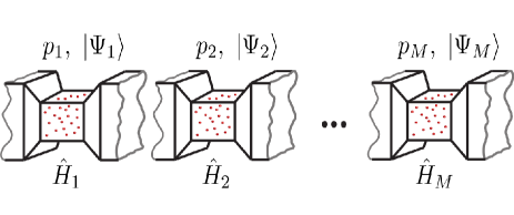
Figure 1: (Color online) If the Hamiltonian depends on microscopic degrees of freedom such as the particle or current density, it is different for each element of the statistical ensemble represented by the probabilities $p_{i}$ that the system is found in the state vector $|\Psi_{i}\rangle$ of $M$ accessible states. A stochastic Hamiltonian precludes the derivation of a closed equation of motion for the density matrix [see discussion following Eq. (19)].

Note that this is true even if the system does not interact with an external environment but its state is mixed. A stochastic Hamiltonian prevents us from writing a closed equation of motion for the density matrix while the SSE (15) contains this case quite naturally: one simply evolves the system dynamics over the ensemble of stochastic Hamiltonians and then averages the resulting dynamics. This point is particularly relevant in DFT where the KS Hamiltonian does depend on microscopic degrees of freedom, and it is thus generally stochastic. Di Ventra and D’Agosta (2007)

There is another important reason for not using the quantum master equation (23) in a DFT approach. In fact, it is only when the Hamiltonian of the system and the bath operators are time-independent that one can prove that the density matrix solution of Eq. (23) fulfills the usual requirements of a “good” statistical operator, i.e., that at any instance of time its trace is conserved, the operator is hermitian and that it remains a definite-positive operator, namely for any state $\Phi$ in the Hilbert space

$$\langle\Phi|\hat{\rho}(t)|\Phi\rangle\geq 0.$$ (24)

The reason for these restrictions is because a dynamical semi-group (in the exact mathematical sense) can only be defined for time-independent Hamiltonians. Lindblad (1976); Maniscalco et al. (2004a, b); Whitney (2008)

It is important to realize that an approach based on the SSE (15) does not suffer from this drawback: the density matrix (21) constructed from the SSE is by definition positive at any time.

All of this points once more to the fact that Eq. (23) is not a good starting point to build a stochastic version of DFT. We will expand a bit more on these issues in Sec. IV. In Sec. VI we will provide an explicit example that shows that Eq. (23) leads to the wrong dynamics in the presence of interactions among particles.

II.4 Continuity equation

We can use the general result Eq. (19) to derive the equation of motion for the ensemble-averaged particle density. Let us define the ensemble-averaged density

$$\overline{n(r,t)}=\langle\overline{{\hat{n}}(r,t)}\rangle,$$ (25)

and current density

$$\overline{j(r,t)}=\langle\overline{\hat{j}(r,t)}\rangle,$$ (26)

where the current operator is defined as

$$\hat{j}(r,t)=\frac{1}{2}\sum_{i}\left\{\delta(r-\hat{r}_{i}),\hat{v}_{i}\right\}$$ (27)

with

$$\hat{v}_{i}=\frac{\hat{p}_{i}+eA_{ext}(\hat{r}_{i},t)}{m},$$ (28)

the velocity operator of particle $i$, and the symbol $\{\hat{A},\hat{B}\}\equiv(\hat{A}\hat{B}+\hat{B}\hat{A})$ is the anti-commutator of any two operators $\hat{A}$ and $\hat{B}$. From Eq. (19) we then get

$$\begin{split}\frac{\partial\overline{n(r,t)}}{\partial t}=&-\nabla\cdot\overline{j(r,t)}\\ &+\frac{1}{2}\overline{\left\langle 2\hat{V}^{\dagger}\hat{n}(r,t)\hat{V}-\hat{V}^{\dagger}\hat{V}\hat{n}(r,t)-\hat{n}(r,t)\hat{V}^{\dagger}\hat{V}\right\rangle}.\end{split}$$ (29)

The last term on the right-hand side of Eq. (29) is identically zero for bath operators that are local in space, Frensley (1990) namely

$$\overline{\left\langle 2\hat{V}^{\dagger}\hat{n}(r,t)\hat{V}-\hat{V}^{\dagger}\hat{V}\hat{n}(r,t)-\hat{n}(r,t)\hat{V}^{\dagger}\hat{V}\right\rangle}\equiv 0.$$ (30)

Most transport theories satisfy this requirement since the action that a true bath does on the system is derived from microscopic mechanisms (e.g., inelastic processes) which are generally local. Frensley (1990) If this were not the case, then this term would represent instantaneous transfer of charge between disconnected – and possibly macroscopically far away – regions of the system without the need of mechanical motion, represented by the first term on the right-hand side of Eq. (29). This instantaneous “action at a distance” is reminiscent of the postulate of wave-packet reduction whereby the system may change its state in a non-unitary way upon measurement.

Here, it is the result of the memory-less approximation that underlies the stochastic Schrödinger equation (15). By assuming that the bath correlation times are much shorter than the times associated with the dynamics of the system (in fact, in the Markov approximation these correlation times are assumed zero), we have lost information on the microscopic interaction mechanisms at time scales on the order of the correlation times of the bath. In other words, we have coarse-grained the time evolution of our system, and we are therefore unable to follow its dynamics on time scales smaller than this time resolution. Gebauer and Car (2004)

In the following, we will assume that the condition (30) is identically satisfied or, if it is not, at any given time, given a physical ensemble-averaged current density, a unique solution for the ensemble-averaged density can be found from Eq. (29).

II.5 Equation of motion for the current density

Similarly, we can derive the equation of motion for the ensemble-averaged current density Di Ventra and D’Agosta (2007)

$$\partial_{t}\overline{j(r,t)} = \frac{\overline{n(r,t)}}{m}\partial_{t}{A_{ext}}({r},t)-\frac{\overline{{j}({r},t)}}{m}\times\left[\nabla\times{A_{ext}}({r},t)\right]$$ (31)

$$+\frac{\langle\overline{\hat{\mathcal{F}}({r},t)}\rangle}{m}+\langle\overline{\hat{\mathcal{G}}({r},t)}\rangle$$

where we have defined

$$\begin{split}\hat{\mathcal{G}}({r},t)&=\hat{V}^{\dagger}\hat{j}({r},t)\hat{V}-\frac{1}{2}\hat{j}({r},t)\hat{V}^{\dagger}\hat{V}-\frac{1}{2}\hat{V}^{\dagger}\hat{V}\hat{j}({r},t),\\ \hat{\mathcal{F}}({r},t)&=-\sum_{i\not=j}\delta({r}-\hat{r}_{i})\nabla_{j}U\left(\hat{r}_{i}-\hat{r}_{j}\right)+m\nabla\cdot\hat{\stackrel{{\scriptstyle\leftrightarrow}}{{\sigma}}}({r},t)\end{split}$$ (32)

with the stress tensor $\hat{\stackrel{{\scriptstyle\leftrightarrow}}{{\sigma}}}({r},t)$ given by

$$\hat{\sigma}_{i,j}({r},t)=-\frac{1}{4}\sum_{k}\{\hat{v}_{i},\{\hat{v}_{j},\delta({r}-\hat{r}_{k})\}\}.$$ (33)

The first two terms on the rhs of Eq. (31) describe the effect of the applied electromagnetic field on the dynamics of the many-particle system; the third is due to particle-particle interactions while the last one is the “force” density exerted by the bath on the system. This last term is responsible for the momentum transfer between the quantum-mechanical system and the environment.

III Stochastic Time-Dependent Current-Density Functional Theory

Having discussed the physical and mathematical requirements for the problem we are interested in, we can now state the following theorem of stochastic time-dependent current-DFT. Di Ventra and D’Agosta (2007)

Theorem: Consider a many-particle system described by the dynamics in Eq. (2) with the many-body Hamiltonian given by Eq. (1). Let $\overline{n({r},t)}$ and $\overline{{j}({r},t)}$ be the ensemble-averaged single-particle density and current density, respectively, with dynamics determined by the external vector potential ${A_{ext}}({r},t)$ and bath operators $\{\hat{V}_{\alpha}\}$. Under reasonable physical assumptions, given an initial condition $|\Psi_{0}\rangle$, and the bath operators $\{\hat{V}_{\alpha}\}$, another external potential $A^{\prime}_{ext}({r},t)$ which gives the same ensemble-averaged current density, must necessarily coincide, up to a gauge transformation, with $A_{ext}({r},t)$.

The details of the proof of this theorem can be found in Ref.  Di Ventra and D’Agosta, 2007. Here, we just mention that the initial condition need not be a pure state for the theorem to be valid, but may include also the case of mixed initial states.

The general idea of the proof, following similar ones proposed by van Leeuwenvan Leeuwen (1999) and VignaleVignale (2004), is to show that the external potential $A^{\prime}_{ext}$ is completely determined, via a power-series expansion in time, by $A_{ext}$, the ensemble-averaged current density, the initial condition, and the bath operators.

A lemma of the theorem states that any ensemble-averaged current density that is interacting $A-$representable is also non-interacting $A-$representable. (A current density is $A-$representable if and only if it can be generated by the application of an external potential $A$.) This implies that if an ensemble-averaged current density can be generated in an interacting system by a given vector potential, then it exists a non-interacting system (the KS system) in which we can obtain the same current density by applying another suitable vector potential, we will call from now on $A_{eff}$.

This is opposed to the general result that an interacting $V-$representable current density (namely one that is generated by a scalar potential $V$) is not necessarily non-interacting $V-$representable. D’Agosta and Vignale (2005) In particular, it has been shown that the mapping between the current density and the scalar potential is not invertible. D’Agosta and Vignale (2005) This result shows that time-dependent DFT does not necessarily provide the exact current density, even if the exact exchange-correlation potential is known (albeit it provides the exact total current for a finite and closed system Di Ventra and Todorov (2004)). With some hindsight this is not surprising since there is clearly no one-to-one correspondence between a scalar and a vector.

III.1 The stochastic Kohn-Sham equations

Let us now assume that we know exactly the vector potential $A_{eff}$ that generates the exact current density in the non-interacting system. By construction, the system follows the dynamics induced by the SSE (for a single bath operator)

$$d|\Psi_{KS}\rangle=\left(-i\hat{H}_{KS}-\frac{1}{2}\hat{V}^{\dagger}\hat{V}\right)|\Psi_{KS}\rangle dt+\hat{V}|\Psi_{KS}\rangle dW$$ (34)

where $|\Psi_{KS}\rangle$ is a Slater determinant of single-particle wave-functions and

$$\hat{H}_{KS}=\sum_{i=1}^{N}\frac{\left[\hat{p}_{i}+eA_{eff}(r_{i},t)\right]^{2}}{2m}$$ (35)

is the Hamiltonian of non-interacting particles.

Note that for a general bath operator acting on many-body wave-functions one cannot reduce Eq. (34) to a set of independent single-particle equations. The reason is that our theorem guarantees that one can decouple the quantum correlations due to the direct interaction among particles, but one cannot generally decouple the statistical correlations induced by the presence of the environment. These affect the population of the single-particle states of the quantum-mechanical system, while the quantum correlations are taken into account to all orders by the external potential $A_{eff}$ acting on the KS system. It is only when the bath operators act on single-particles or on the density that one can write Eq. (34) as a set of equations of motion, one for every KS single-particle state. Bushong and Di Ventra (2007)

III.2 Initial conditions

The initial condition for the time evolution of the KS system has to be chosen such that the ensemble-averaged particle and current densities coincide with those of the many-body interacting system. Again, it is important to stress that in going from the interacting system to its non-interacting doppelgänger, the bath operator is not modified. On the other hand, the bath operator $\hat{V}$ generally induces transitions between many-body states of the interacting Hamiltonian (1). Therefore, when represented in the non-interacting basis of the KS Hamiltonian it may connect many different single-particle KS states. It has been argued that this way the KS system will never reach a stationary state even if the coupling with the environment is purely dissipative. Burke et al. (2005) It would be thus tempting to modify the bath operator to force the KS system into an equilibrium with the external environment. Burke et al. (2005) This procedure, however, breaks the theorem we have proved, and contains approximations of unknown physical meaning.

In reality, if the true many-body system reaches equilibrium with the environment, then the ensemble-average current and particle density would attain a stationary limit. Since, these are the only two physical quantities that the KS system needs to reproduce, the question of whether the latter is in equilibrium with the environment or not has no physical relevance.

III.3 The exchange-correlation vector potential

The vector potential $A_{eff}(r,t)$, acting on the KS system is generally written as the sum of two contributions

$$A_{eff}(r,t)=A_{ext}(r,t)+A_{h-xc}(r,t),$$ (36)

where $A_{ext}(r,t)$ is the vector potential applied to the true many-body system, and $A_{h-xc}(r,t)$ is the vector potential whose scope is to mimic the correct dynamics of the ensemble-averaged current density. From the theorem we have proven, $A_{h-xc}(r,t)$ is a functional of the average current density $\overline{j(r,t^{\prime})}$, for $t^{\prime}\leq t$ (namely, it is history-dependent), the initial condition and the bath operator $\hat{V}$. Di Ventra and D’Agosta (2007)

A common expression would isolate from $A_{h-xc}(r,t)$ the Hartree interaction contribution from the “rest” due to the particle exchange and correlation, namely one makes the ansatz

$$A_{h-xc}(r,t)=A_{h}(r,t)+A_{xc}(r,t)$$ (37)

where $A_{h}(r,t)$ is the Hartree contribution to the vector potential ($t_{0}$ is the initial time)

$$A_{h}(r,t)=\int_{t_{0}}^{t}dt^{\prime}\nabla\int dr^{\prime}\frac{\overline{n(r^{\prime},t^{\prime})}}{|r-r^{\prime}|}.$$ (38)

The other contribution, $A_{xc}(r,t)$ is again a functional of the average current density $\overline{j(r,t^{\prime})}$, for $t^{\prime}\leq t$, the initial condition, and the bath operator $\hat{V}$,Di Ventra and D’Agosta (2007)

$$A_{xc}(r,t)=A_{xc}\left[\overline{j(r,t^{\prime})},|\Psi_{0}\rangle,\hat{V}\right].$$ (39)

In the present case, however, particular care needs to be applied to the above ansatz. We have written the Hartree contribution in terms of the ensemble-averaged density. This choice, however, requires that the exchange-correlation vector potential included also the statistical correlations of the direct Coulomb interaction at different points in space. These correlations may be very large, and possibly much larger than the Coulomb interaction between the average densities. The ambiguity here, compared to the pure-state case, is because in a mixed state, quite generally the ensemble-average of the direct Coulomb interaction energy contains statistical correlations between densities at different points in space, namely

$$\int dr\int dr^{\prime}\frac{\overline{\langle\hat{n}(r)\rangle\,\langle\hat{n}(r^{\prime})\rangle}}{|r-r^{\prime}|}\neq\int dr\int dr^{\prime}\frac{\langle\overline{\hat{n}(r)}\rangle\;\langle\overline{\hat{n}(r^{\prime})}\rangle}{|r-r^{\prime}|}.$$ (40)

In actual calculations, one would instead use the form of the Hartree potential in terms of the density per element of the ensemble. This choice (38) makes the KS Hamiltonian (35) stochastic, and therefore, as discussed in Sec. II, no closed equation of motion for the many-particle KS density matrix can be obtained.

Finally, in view of the fact that one can derive a Markovian dynamics only on the basis of a weak interaction with the environment,Van Kampen (2001); Gardiner (1983) as a first approximation, one may neglect the dependence of the exchange-correlation vector potential on the bath operator, and use the standard functionals of TD-DFT and TD-CDFT.Marques et al. (2006); Vignale and Kohn (1996) [Like the Hartree term, these functionals would also contribute to the stochasticity of the KS Hamiltonian (35).] This seems quite reasonable, but only comparison with experiments and the analysis of specific cases can eventually support it. We thus believe that more work in this direction will be necessary.

IV Connection with a density-matrix approach

From the KS Slater determinants $|\Psi^{i}_{KS}\rangle$, solutions of the KS equation (34) occurring with weight $p_{i}(t)$ ($\sum_{i}p_{i}(t)=1$) in the ensemble, we can construct the many-particle KS density matrix [from Eq. (20)]

$$\hat{\rho}_{KS}(t)=\overline{|\Psi^{i}_{KS}(t)\rangle\langle\Psi^{i}_{KS}(t)|}\equiv\sum_{i}\,p_{i}(t)\,|\Psi^{i}_{KS}(t)\rangle\langle\Psi^{i}_{KS}(t)|.$$ (41)

This density matrix is, by construction, always positive-definite, despite the fact that the KS Hamiltonian and possibly the $\hat{V}$ operator are time dependent. Since in general the bath operator acts on many-particle states, this many-particle KS density matrix cannot be reduced to a set of single-particle density matrices (see Sec. V for a numerical ansatz suggested in Ref. Pershin et al., 2008 to simplify the calculations).

We note first that, in principle, if we knew the exact functional $A_{h-xc}$ as a functional of the averaged current density, then the KS Hamiltonian (35) would not be stochastic and we could derive the equation of motion of the many-particle KS density matrix (41). This equation of motion would be Eq. (23) with $\hat{H}$ replaced by $\hat{H}_{KS}$.

It is important to point out, however, that it is only when we start from the stochastic KS equation (34) to construct the density matrix (41) that we are guaranteed that the solution of Eq. (23) for the KS density matrix maintains positivity at any time. The reverse is not necessarily true: the equation of motion (23) for the KS density matrix may, for an arbitrary bath operator $\hat{V}$ or initial conditions, provide non-physical solutions. In other words, Eq. (23) admits more solutions than physically allowed, while the SSE always provides a physical state of the system dynamics.

We also stress once more that any approximation to $A_{h-xc}$, makes the KS Hamiltonian stochastic, namely one Hamiltonian for each element of the ensemble, thus making the density-matrix formalism of limited value. In fact, by insisting on using Eq. (23) with these approximations would amount to introducing uncontrollable approximations in the system dynamics which entail neglecting important statistical correlations induced by the bath (see also discussion in Sec. VI).

To see this point explicitly, let us consider the equation of motion for an arbitrary operator acting on the KS system that evolves according to Eq. (17) with $\hat{H}_{KS}$ replacing $\hat{H}$

$$\begin{split}d\langle\hat{A}\rangle=&\left\langle i[\hat{A},\hat{H}_{KS}]-\frac{1}{2}\left(\hat{V}^{\dagger}\hat{V}\hat{A}+\hat{A}\hat{V}^{\dagger}\hat{V}-2\hat{V}\hat{A}\hat{V}^{\dagger}\right)\right\rangle dt\\ &+\langle\hat{V}^{\dagger}\hat{A}+\hat{A}\hat{V}\rangle dW.\end{split}$$ (42)

Now we take the ensemble average of this equation in order to obtain the equation of motion for the ensemble-averaged quantities. However, since now $H_{KS}$ is a stochastic Hamiltonian, then the ensemble average and the commutator between $\hat{A}$ and $\hat{H}_{KS}$ do not commute, i.e., in general we expect that

$$\overline{[\hat{A},\hat{H}_{KS}]}\not\equiv[\overline{\hat{A}},\hat{H}_{KS}],$$ (43)

which implies that

$$\begin{split}\partial_{t}\hat{\rho}_{KS}\neq&-i\left[\hat{\rho}_{KS},\hat{H}_{KS}\right]\\ &-\frac{1}{2}\left(\hat{V}^{\dagger}\hat{V}\hat{\rho}_{KS}+\hat{\rho}_{KS}\hat{V}^{\dagger}\hat{V}-2\hat{V}\hat{\rho}_{KS}\hat{V}^{\dagger}\right),\end{split}$$ (44)

namely there is no closed equation of motion for the KS density matrix.

In fact, the correct procedure is to evolve the system for every realization of Hamiltonians, and then average over these realizations, which is what a solution of the SSE (34) would provide.

V Numerical solution of the SSE

V.1 Finite difference equation

We now discuss practical implementations of the SSE (34). First of all we realize that, in going from the differential equation (34) to a finite difference equation that can be solved on a computer, one has to bear in mind that $dW$ is on the order of $\sqrt{dt}$. Then one has to expand the equation for the finite differences and keep terms of second order in $dW$ that correspond to first order in $dt$.

Here we write down the correct finite difference equation starting from (34). In the following we assume that the state vector $\Psi_{KS}$ is a regular function of time, position, and the Wiener process $W$, i.e., we assume that the derivatives

$$\frac{\partial\Psi_{KS}}{\partial W},~{}~{}\frac{\partial^{2}\Psi_{KS}}{\partial W\partial W},~{}\ldots$$ (45)

exist and are regular.

Let us define $dt=t-t^{\prime}$ a small time interval over which we integrate the equation of motion for $\Psi_{KS}$. If we expand in series the increment $d\Psi_{KS}=\Psi_{KS}(t)-\Psi_{KS}(t^{\prime})$ we have,

$$d\Psi_{KS} = \frac{\partial\Psi_{KS}}{\partial t}dt+\frac{\partial\Psi_{KS}}{\partial W}dW+\frac{1}{2}\frac{\partial^{2}\Psi_{KS}}{\partial W\partial W}dWdW+\ldots$$ (46)

$$= \left(\frac{\partial\Psi_{KS}}{\partial t}+\frac{1}{2}\frac{\partial^{2}\Psi_{KS}}{\partial W\partial W}\right)dt+\frac{\partial\Psi_{KS}}{\partial W}dW.$$

A direct term-by–term comparison with Eq. (34) tells us that there is a correspondence between $\partial/{\partial W}$ and $\hat{V}$ so that a finite difference scheme can now be implemented such that the equation of motion

$$\Delta\Psi_{KS} = \left(\frac{\partial\Psi_{KS}}{\partial t}\right)\Delta t+\left(\frac{\partial\Psi_{KS}}{\partial W}\right)\Delta W$$ (47)

$$= \left(-iH_{KS}-\frac{1}{2}V^{\dagger}V-\frac{1}{2}\hat{V}^{2}\right)\Psi_{KS}\Delta t$$

$$+\hat{V}\Psi_{KS}\Delta W,$$

is the correct first-order equation in $\Delta t$. Eq. (47) can now be solved by a variety of different numerical techniques, and we refer the reader to other work for a discussion of such methods.Kloeden et al. (1997); Breuer and Petruccione (2002); Wilkie (2004); Wilkie and Cetinbas (2005)

The important point is that one evolves these equations in time for every realization of the stochastic process and then averages over the different realizations (in Sec. VI we give an explicit example of such calculation showing the convergence of the results with the number of realizations).

V.2 The non-linear SSE

The norm of the state vector solution of the SSE (34) is preserved on average but not for every realization of the stochastic process.Van Kampen (2001); Di Ventra and D’Agosta (2007) This may slow down the convergence of the results as a function of the number of realizations of the stochastic process. It is thus more convenient to solve a non-linear SSE which gives an equivalent solution as the linear SSE (34). This can be easily done by first calculating the differential [in the Itô sense (7)] of the square modulus of $|\Psi_{KS}\rangle$

$$d||\Psi_{KS}||^{2} = \langle\Psi_{KS}|(\hat{V}^{{\dagger}}+\hat{V})|\Psi_{KS}\rangle dW$$ (48)

$$\equiv 2R\,||\Psi_{KS}||^{2}dW,$$

where we have defined

$$R=\frac{1}{2}\frac{\langle\Psi_{KS}|(\hat{V}^{{\dagger}}+\hat{V})|\Psi_{KS}\rangle}{||\Psi_{KS}||^{2}}.$$ (49)

By using the power expansion

$$d||\Psi_{KS}|| = d\sqrt{||\Psi_{KS}||^{2}}$$ (50)

$$= \frac{1}{2\sqrt{||\Psi_{KS}||^{2}}}d||\Psi_{KS}||^{2}$$

$$-\frac{1}{8(\sqrt{||\Psi_{KS}||^{2}})^{3}}d||\Psi_{KS}||^{2}d||\Psi_{KS}||^{2},$$

we can derive the equation of motion for the state vector normalized at every realization of the stochastic process:

$$|\Phi_{KS}\rangle=\frac{|\Psi_{KS}\rangle}{||\Psi_{KS}||}$$ (51)

which is (see also Ref. Ghirardi et al., 1990)

$$d|\Phi_{KS}\rangle = \left[-i\hat{H}_{KS}-\frac{1}{2}\hat{V}^{{\dagger}}\hat{V}+R\hat{V}-\frac{1}{2}R^{2}\hat{1}\right]|\Phi_{KS}\rangle dt$$ (52)

$$+(\hat{V}-R\hat{1})|\Phi_{KS}\rangle dW.$$

This non-linear equation of motion, by construction, is equivalent to the linear SSE (34).

The finite-difference equation for this case is

$$\Delta\Phi_{KS} = \left(\frac{\partial\Phi_{KS}}{\partial t}\right)\Delta t+\left(\frac{\partial\Phi_{KS}}{\partial W}\right)\Delta W$$ (53)

$$= \left(-iH_{KS}-\frac{1}{2}V^{\dagger}V-\frac{1}{2}\hat{V}^{2}+R\hat{V}-\frac{1}{2}R^{2}\hat{1}\right)\Phi_{KS}\Delta t+(\hat{V}-R\hat{1})\Phi_{KS}\Delta W.$$

V.3 Single-particle order-$N$ scheme

Due to the presence of the environment, it is still a formidable task to solve the equations of motion of S-TDCDFT for arbitrary bath operators. In fact, as we have already discussed, the bath operators generally act on Slater determinants and not on single-particle states. If we have $N$ particles and retain $M$ single-particle states, this requires the solution of $C_{N}^{M}-1$ elements of the state vector (with $C_{N}^{M}=M!/N!(M-N)!$ and the $-1$ comes from the normalization condition). In addition, one has to average over an amount, call it $m$, of different realizations of the stochastic process.  The problem thus scales exponentially with the number of particles.

However, it was recently suggested in Ref. Pershin et al., 2008 that for operators of the type $\hat{A}=\sum_{j}\hat{A}_{j}$, sum over single-particle operators (like, e.g., the density or current density), the expectation value of $\hat{A}$ over a many-particle non-interacting state with dissipation can be approximated as a sum of single-particle expectation values of $\hat{A}_{j}$ over an ensemble of $N$ single-particle systems with specific single-particle dissipation operators. In particular, the agreement between the exact many-body calculation and the approximate single-particle scheme has been found to be excellent for the current density. Pershin et al. (2008) We refer the reader to Ref. Pershin et al., 2008 for the numerical demonstration of this scheme and its analytical justification. The physical reason behind it is that, due to the coupling between the system and the environment, highly-correlated states are unlikely to form.

Here, for numerical convenience, we will adopt the same ansatz which in the present case reads,

$$\overline{\langle\Psi_{KS}|\hat{A}|\Psi_{KS}\rangle}\simeq\sum_{j=1}^{N}\overline{\langle\phi^{j}_{KS}|\hat{A}_{j}|\phi^{j}_{KS}\rangle},$$ (54)

with $|\phi^{j}_{KS}\rangle$ single-particle KS states solutions of

$$d|\phi^{j}_{KS}\rangle = \left[-i\frac{\left(\hat{p}+eA_{eff}(r,t)\right)^{2}}{2m}-\frac{1}{2}\hat{V}_{sp}^{\dagger}\hat{V}_{sp}\right]|\phi^{j}_{KS}\rangle dt$$ (55)

$$+\hat{V}_{sp}|\phi^{j}_{KS}\rangle dW(t),$$

with $\hat{V}_{sp}$ an operator acting on single particle states (see Refs. Pershin et al., 2008 and Bushong and Di Ventra, 2007 and next section for explicit examples of such operator). 

For convenience, also in the present case we can normalize the single-particle KS states for every realization of the stochastic process by defining

$$|\tilde{\phi}^{j}_{KS}\rangle=\frac{|\phi^{j}_{KS}\rangle}{||\phi^{j}_{KS}||}$$ (56)

and thus solve the non-linear SSE

$$d|\tilde{\phi}^{j}_{KS}\rangle = \left[-i\frac{\left(\hat{p}+eA_{eff}(r,t)\right)^{2}}{2m}-\frac{1}{2}\hat{V}_{sp}^{\dagger}\hat{V}_{sp}\right.$$ (57)

$$\left.+R_{j}\hat{V}_{sp}-\frac{1}{2}R_{j}^{2}\hat{1}\right]|\tilde{\phi}^{j}_{KS}\rangle dt$$

$$+(\hat{V}_{sp}-R_{j}\hat{1})|\tilde{\phi}^{j}_{KS}\rangle dW(t),$$

where

$$R_{j}=\frac{1}{2}\frac{\langle\phi^{j}_{KS}|(\hat{V}_{sp}^{{\dagger}}+\hat{V}_{sp})|\phi^{j}_{KS}\rangle}{||\phi^{j}_{KS}||^{2}}.$$ (58)

The discretization of these equations is then done similarly to what we have explained in the previous section.

VI An example: A gas of linear harmonic oscillators

Stochastic-TDCDFT has been applied to the study of decay of exited He atoms and its connection to quantum-measurement theory.Bushong and Di Ventra (2007) It can describe the dynamics of bosons as well. In this section, we apply it to the analysis of the dynamics of an interacting 1D Bose gas confined in a harmonic potential and coupled to a uniform external environment that forces the gas towards some steady state. Since neither the external potential nor the bath are time-dependent, we expect that the boson gas reaches a steady state configuration when coupled with the uniform external bath. Finally, we assume that the bath forces the system towards certain eigenstates of the instantaneous interacting boson Hamiltonian. The bosons are interacting via a two-body contact potential, i.e., $U_{int}(x,x^{\prime})\propto\delta(x-x^{\prime})$. This potential correctly describes the important case of Alkali gases in which the Bose-Einstein condensation has been experimentally observed. Davis et al. (1995); Anderson et al. (1995); Dalfovo et al. (1999)

The purpose of this section is to compare the dynamics of the boson gas obtained from the SSE [Eq.(15)] and the quantum master equation [Eq. (23)]. For this reason the value of the physical parameters (the strengths of the confining potential, the particle-particle interaction, and the system-bath coupling) is arbitrary and chosen only for the sake of this comparison. We will report elsewhere a more realistic study of the dynamics of this important physical system. When no interaction between particles is included both approaches are clearly equivalent. However, when interactions are included, the Hamiltonian of the system becomes stochastic and, as previously discussed, the quantum master equation does not take into account correctly the statistical correlations induced by the bath, while the SSE naturally accounts for the the stochasticity introduced in the Hamiltonian by the interaction potential. In fact, we find that when both the initial and final state are pure, both approaches provide the same equilibrium state. However, the corresponding dynamics are different. In particular, the relaxation time obtained from the evolution of the density matrix is shorter than the relaxation time obtained from the average over many realizations of the dynamics obtained from the SSE.

The differences between the two approaches are even more striking when we consider the evolution towards a state that contains at least two major contributions coming from different states. In this case, also the final steady states obtained from the density matrix and the SSE are different.

These cases exemplify what we have discussed all along: if one insists on using a closed equation of motion for the density matrix of the type (23) with stochastic Hamiltonians, uncontrolled approximations are introduced which lead to an incorrect dynamics.

VI.1 Macroscopic occupation of the ground state

We begin with the study of the dynamics of the macroscopic occupation of the ground state induced by energy dissipation towards the degrees of freedom of an external bath. The external bath forces the system to reach a state of zero temperature or minimal free energy, i.e., the ground state of the Hamiltonian. One possible form of this bath operator is, in a basis set that makes the Hamiltonian diagonal at each instance of time, Bushong and Di Ventra (2007)

$$\hat{V}\equiv\delta\left(\begin{array}[]{ccccc}0&1&1&1&\ldots\\ 0&0&0&0&\ldots\\ \vdots&\vdots&\vdots&\vdots&\vdots\\ 0&0&0&0&\ldots\end{array}\right),$$ (59)

where $\delta$ is a coupling constant with dimensions of the square root of a frequency [we set $\delta=\sqrt{\omega_{0}}$ in what follows, with $\omega_{0}$ the frequency of the harmonic confining potential – see Eq. (63)]. We do not expect that this operator fulfills Eq.(30) since in a real-space representation it would allow for the localization of the particles without an effective current between two distinct points in space. In this section, however, we are more interested in the kind of dynamics this operator generates in our quantum system, and the comparison with the dynamics obtained from the quantum master equation. We expect, indeed, that the condition Eq.(30) is violated both in the SSE and in the quantum master dynamics.

The operator (59) mimics the energy dissipation in the system, with the external bath absorbing the bosons’ excess energy and cooling down the boson gas. One could argue that this is the generalization to the many-state system of the bath considered in Ref. (Van Kampen, 2001). We can thus conclude that the effective temperature of the bath we consider here is zero.

The Hamiltonian of the boson system (in second quantization) when the bath is not present reads

$$\hat{H} = \int dx~{}\psi^{\dagger}(x)\left(-\frac{1}{2m}\frac{d^{2}}{dx^{2}}+V_{ext}(x)\right)\psi(x)$$ (60)

$$+\int dxdx^{\prime}~{}\psi^{\dagger}(x)\psi^{\dagger}(x^{\prime})U_{int}(x-x^{\prime})\psi(x^{\prime})\psi(x),$$

where $\psi(x)$ destroys a boson at position $x$, $V_{ext}(x)$ is a confining potential, and $U_{int}(x-x^{\prime})$ is the boson-boson interaction potential. For dilute boson atomic gases the interaction potential can be substituted with the contact potential, i.e.,

$$U_{int}(x-x^{\prime})=g_{0}(N-1)\delta(x-x^{\prime})=\tilde{g}\delta(x-x^{\prime})$$ (61)

where $g_{0}$ is determined by the scattering length of the boson-boson collision in the dilute gas, and $N$ is the total number of bosons in the trap, so that $||\psi||$=1.Dalfovo et al. (1999)

With standard techniques, and in the Hartree approximation, we can go from the equation of motion for the annihilation operators to the equation of motion for the state of the system $\Psi(x,t)$, when the external bath is not coupled to the boson gas,

$$i\partial_{t}\Psi(x,t)=\left[-\frac{1}{2m}\frac{d^{2}}{dx^{2}}+V_{ext}(x)\right]\Psi(x,t)+\tilde{g}n(x,t)\Psi(x,t)$$ (62)

where $n(x,t)=|\Psi(x,t)|^{2}$ is the single-particle density of the boson gas.Gross (1963); Ginzburg and Pitaevskii (1958)

Equation (62) (and its generalization to 2 and 3 dimensions) has received a lot of attention since it correctly describes the dynamics of a Bose-Einstein condensate.Davis et al. (1995); Anderson et al. (1995); Dalfovo et al. (1999)

In the following we will focus on the case of a 1D harmonic confining potential, i.e.,

$$V_{ext}(x)=\frac{1}{2}m\omega_{0}^{2}x^{2}.$$ (63)

A harmonic confinement is created, e.g., in the magneto-optical traps used in the experimental realization of the Bose-Einstein condensation of dilute boson Alkali gases.Davis et al. (1995); Anderson et al. (1995); Dalfovo et al. (1999)

When the boson system is coupled to the external environment, we assume that the Hamiltonian is not affected by the coupling and the state of the system $\Psi(x,t)$, that is now stochastic, evolves according to the SSE

$$d\Psi(x,t)=-i\left(-\frac{1}{2m}\frac{d^{2}}{dx^{2}}+\frac{1}{2}m\omega_{0}^{2}x^{2}+gn(x,t)\right)\Psi(x,t)dt-\frac{1}{2}\hat{V}^{\dagger}\hat{V}\Psi(x,t)dt+\hat{V}\Psi(x,t)dW$$ (64)

where this equation of motion has to be interpreted in accordance to the discussion of the previous Sections. For numerical convenience, we rescale this equation in terms of the physical quantities $\omega_{0}$, $x_{0}=1/\sqrt{m\omega_{0}}$, and $g=\tilde{g}/x_{0}$ to arrive at

$$d\Psi(x,t)=-i\omega_{0}\left(-\frac{x_{0}^{2}}{2}\frac{d^{2}}{dx^{2}}+\frac{x^{2}}{2x_{0}^{2}}+\frac{g}{\omega_{0}}n(x,t)x_{0}\right)\Psi(x,t)dt-\frac{1}{2}\hat{V}^{\dagger}\hat{V}\Psi(x,t)dt+\hat{V}\Psi(x,t)dW.$$ (65)

We begin by considering the case of non-interacting bosons, i.e., we set $g=0$. In this case, the Hamiltonian admits a natural complete basis, the set of Hermite-Gauss wave-functions

$$\varphi_{j}(x)=\frac{1}{\sqrt{x_{0}2^{j}j!\sqrt{\pi}}}H_{j}(x/x_{0})e^{-x^{2}/2x_{0}^{2}}$$ (66)

where the polynomials $\{H_{j}\}$ satisfy the recursion relation

$$H_{j+1}(x)=2xH_{j}(x)-H_{j-1}$$ (67)

and $H_{0}(x)=1$, $H_{1}(x)=2x$. If we expand the wave-function $\Psi(x,t)=\sum_{j}a_{j}(t)\varphi_{j}(x)$, and make use of the orthonormality properties of the Hermite-Gauss wave-functions, we obtain the (stochastic) dynamical equation for the coefficients $a_{j}$,

$$da_{i}=\sum_{j}\left(H_{ij}a_{j}+\frac{1}{2}(\hat{V}^{\dagger}\hat{V})_{ij}a_{j}\right)dt+dW\sum_{j}\hat{V}_{ij}a_{j}$$ (68)

where $H_{ij}=(j+1/2)\omega_{0}\delta_{ij}$ and $\hat{V}$ is given by Eq. (59).

Together with Eq. (68) we can study the dynamics of the density matrix via the quantum master equation Eq. (23), which in the same spatial representation as Eq. (68) reads

$$\partial_{t}\rho_{ij}=-i\sum_{k}\left(H_{ik}\rho_{kj}-\rho_{ik}H_{kj}\right)+\sum_{k,k^{\prime}}\left(\hat{V}_{ik}\rho_{kk^{\prime}}\hat{V}^{\dagger}_{k^{\prime}j}-\frac{1}{2}\hat{V}^{\dagger}_{ik}\hat{V}_{kk^{\prime}}\rho_{k^{\prime}j}-\frac{1}{2}\rho_{ik}\hat{V}^{\dagger}_{kk^{\prime}}\hat{V}_{k^{\prime}j}\right),$$ (69)

The connection between Eq. (68) and Eq. (69) is established by the identity $\rho_{ij}=a^{*}_{i}a_{j}$ valid for any pair of indexes $i$ and $j$. We solve Eq. (68) numerically with a 4th order Runge-Kutta evolution scheme, after we have mapped the dynamics to its norm-preserving equivalent form (see Sec. V and the discussion therein).Ghirardi et al. (1990); Breuer and Petruccione (2002) For consistency we solve the master equation with a 2nd order Runge-Kutta evolution scheme (in fact with the more refined Heun’s scheme).Press et al. (1992)

We report in Fig. (2) the dynamics of the probability of occupation of the ground state, $p_{0}=|a_{0}|^{2}=\rho_{00}$ for various realizations of the stochastic field in Eq. (68) together with the dynamics obtained from the evolution of the density matrix (69). Here, we have included the first 20 levels of the free Hamiltonian, and we have chosen as initial condition $a_{20}(0)=1$ and set the other coefficients to zero.

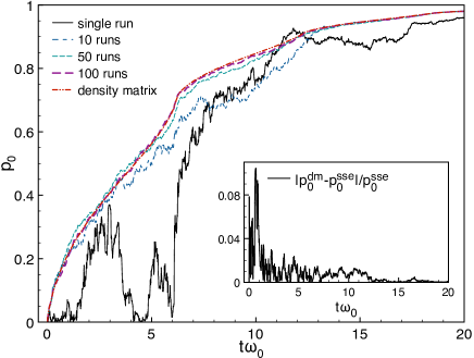
Figure 2: (Color online) Non-interacting bosons – Occupation probability of the ground state versus time calculated from the evolution of the state via the SSE averaged over different runs (1, 10, 50 and 100) and via the equation of motion for the density matrix for the non-interacting boson case. It is evident that with only 50 realizations the agreement between the SSE and the density matrix equation is excellent. In the inset we show the relative difference between the two dynamics for 100 realizations of the stochastic process.

We have set the mass of the particles to $1$, and used a time step $\omega_{0}\Delta t=20/2^{15}=6\times 10^{-4}$. A further decrease of this time step does not affect the results significantly. From Fig. 2, it is evident that when we collect a large enough statistics the results of the SSE and the master equation coincide for the non-interacting boson case: Already for 50 runs of the SSE the difference between the two dynamics almost vanishes. In the inset of Fig. 2 we report the relative difference between the occupation number of the ground state with the two dynamics, $|p_{0}^{dm}-p_{0}^{sse}|/p_{0}^{sse}$. We see that this difference, for 100 runs, is generally lower than $5\%$, a quite satisfactory result.

In Fig. 3, we report the density profile for the system at different instances of time obtained from the SSE. Starting from a pure state, where the highest energy state is occupied (panel $c$), the system relaxes towards the ground state. As it is clear from panel $a)$ in Fig. 3 the system, at $t\omega_{0}=20$, still occupies certain high energy states [see, e.g., the tail at $x<0$ of panel $a)$].

Figure 3: Non-interacting bosons – Plot of the averaged density profile, $n(x)\times x_{0}^{2}$, for various instances of time calculated from the SSE. The system evolves from the maximum occupation of the highest excited state (panel c), to the maximum occupation of the ground state. We have averaged over 100 realizations of the stochastic process.

We now turn on the particle-particle interaction $U_{int}$. This corresponds to adding to the free Hamiltonian $H_{i,j}$ an interaction part, $H^{int}$ that in the basis representation of the Gauss-Hermite polynomials reads

$$H^{int}_{i,j}=\sum_{k,q}F_{i,j;k,q}a_{k}^{*}a_{q}$$ (70)

where $F_{i,j;k,q}$ is the 4th-rank tensor defined as

$$F_{i,j;k,q}=g\int_{-\infty}^{\infty}dx~{}H_{i}(x)H_{j}(x)H_{k}(x)H_{q}(x)e^{-2x^{2}}.$$ (71)

A long but straightforward calculation brings us to an explicit expression of $F_{i,j;k,q}$ in terms of Euler gamma functions and a hypergeometric function.Lord (1949); Abramowitz and Stegun (1964) It can be shown that the hypergeometric function reduces to the summation of a few – at most $\min(i,j)$ – terms. In the case of the density matrix approach the interaction Hamiltonian is immediately written as

$$H^{int}_{i,j}=\sum_{k,q}F_{i,j;k,q}\rho_{k,q}.$$ (72)

In solving the dynamics of the system described either by the SSE (65) or the master equation (69), we have assumed that at any instance of time the bath operator brings the system towards the instantaneous ground state of the interacting Hamiltonian $H_{i,j}+H_{i,j}^{int}$.

In Fig. 4 we plot the occupation probability $p_{j}(t)$ of the state $j$ for the first 3 levels of the free Hamiltonian ($p_{j}(t)=|a_{j}(t)|^{2}$ from the SSE or $p_{j}(t)=\rho_{j,j}(t)$ from the density matrix). We have assumed an interaction of strength $g/\omega_{0}=5$, and a time step $\omega_{0}\Delta t=60/2^{17}$ and we have performed 100 independent runs of the SSE. While it evident that the system reaches the same steady state according to the two equations,  it is also clear that the state calculated with the SSE relaxes slower than the state obtained from the density matrix equation. This is a spurious effect in the density matrix dynamics where the average density defines the interaction potential. This does not take into account the fluctuations of the state, and hence of the stochastic Hamiltonian.

We have also tested that the steady state reached during the dynamics is consistent with the theory of the eigenstates of the Gross-Pitaevskii equation. D’Agosta and Presilla (2000); Dalfovo et al. (1999) In particular, the ground state of the interacting system, when the interaction is strong, can be obtained by neglecting the kinetic contribution to the Hamiltonian. In this case, a good approximation to the ground state density reads

$$|\Psi_{0}(x)|^{2} = \frac{\mu-1/2m\omega_{0}^{2}x^{2}}{gx_{0}}\theta\left(\mu-1/2m\omega_{0}^{2}x^{2}\right)$$ (73)

$$+\mathrm{terms~{}proportional~{}to}~{}1/g^{2}$$

where $\mu$, the chemical potential, is determined by the normalization condition, and $\theta(x)=0$ if $x<0$ and $\theta(x)=1$ if $x>0$.

In the inset of Fig. 4 we plot the density obtained at $t\omega_{0}=60$ from the SSE (black, dashed line) and the density obtained from the approximation (73) (orange, solid line). Notice that the value of the parameters $g$ and $\mu$ have been obtained from the best fit with the numerics: indeed one can show that the approximation (73) is exact in the limit of very large interaction,D’Agosta and Presilla (2000); Dalfovo et al. (1999) which is not reached in our calculations.

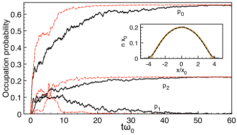
Figure 4: (Color online) Interacting bosons – Occupation probability of the first 3 lowest energy levels of the non-interacting Hamiltonian versus time calculated via the SSE (black, solid lines) averaged over 100 independent runs, and via the equation of motion for the density matrix (red, dashed lines). The time it takes the system to reach steady state is different for the density matrix approach and the SSE, with the former underestimating the relaxation time. This is due to the inclusion in the master equation of the average density in the interaction potential, thus neglecting important fluctuations that can slow down the relaxation dynamics. In the inset we compare the equilibrium density (black, dashed line) with the one obtained from the Thomas-Fermi approximation to the ground state (orange, solid line).

In Fig. 5 we report the value of the ground state energy of the interacting Hamiltonian versus time as calculated from the SSE and the master equation. Again the difference between the relaxation times calculated from the two dynamics is evident. In the inset of Fig. 5 we report the energy of the first excited state.

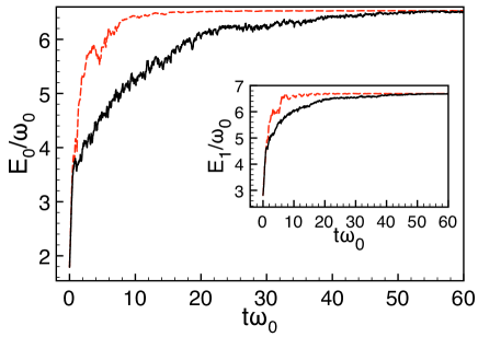
Figure 5: (Color online) Interacting bosons – Time evolution of the energy of the ground state of the Gross-Pitaevskii Hamiltonian as calculated from the SSE (black, solid line) and master equation (red, dashed line). The final value of the energy is the same, but the relaxation dynamics is different in the two formalisms with the master equation considerably underestimating the relaxation time. In the inset we report the dynamics of the first excited state of the Gross-Pitaevskii Hamiltonian obtained from the SSE (black, solid line) and the master equation (red, dashed line).

To summarize this section, we have described the dynamics of the relaxation of a confined 1D boson system towards the ground state induced by a given external bath. The final state we have obtained is consistent with the eigenstate of the 1D Gross-Pitaevskii equation. Our main result is that, although the SSE and the master equation reach the same final state, the dynamics described by these equations show important differences, and physical quantities, like, e.g., the relaxation time, differ. In particular, the density matrix approach, which at any instant of time employs the average density to construct the interaction Hamiltonian, underestimates the fluctuations induced by the bath on the stochastic Hamiltonian. These fluctuations are correctly taken into account in the SSE.

VI.2 Competition between states

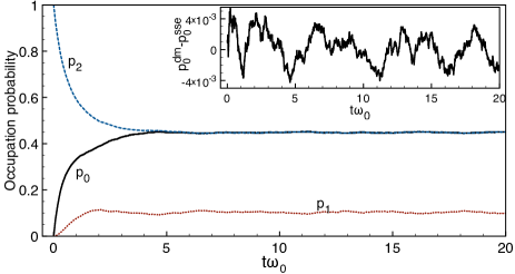
Figure 6: (Color online) Non-interacting bosons – The occupation probabilities for a three level system calculated via the SSE (65) for non-interacting bosons ($g=0$). The results obtained via the master equation for the density matrix are indistinguishable on this scale from those obtained with the SSE. In the inset we show the difference between the occupation probabilities of the lowest energy level calculated from the SSE and the master equation. This difference is in modulus lower than $5\times 10^{-3}$ at any instant of time.

Let us now consider the more common case in which the environment drives the system toward a mixed steady state. To simplify the discussion we consider only three single-particle levels and the bath operator forces the system towards two different states. We choose, in a basis in which the Hamiltonian is diagonal, the operator

$$V=\delta\left(\begin{array}[]{ccccc}0&1&1\\ 0&0&0\\ 1&1&0\end{array}\right),$$ (74)

i.e., the operator drives the system, with equal strength, towards the lowest and highest energy levels of the interacting Hamiltonian. As we will see, the final state is a superposition of these two states with a significant contribution coming from the middle level. At first glance this might seem surprising. However, we have to remember that, e.g., in the quantum master equation, the equilibrium states are determined by the kernel of the super-operator. This super-operator contains powers of the operator $V$, that in turn contains a finite contribution from the middle level. A similar reasoning applies to the SSE.

To begin with our analysis of this system, we consider the non-interacting case $g=0$; we set as before $\delta=\sqrt{\omega_{0}}$; and we start from the fully occupied highest energy level, i.e., $a_{3}(0)=1$. In Fig. 6 we plot the occupation probabilities for the 3 levels calculated via the SSE (65). In this case, to reduce the stochastic noise even further, we have performed 1000 independent runs of the SSE and used, in both dynamics, $\omega_{0}\Delta t=20/2^{14}$. As we can see from Fig. 6, at steady state the bath operator forces the system to occupy the lowest and the highest energy levels with equal probability, while a finite occupation probability of the middle level appears. This mixing prevents the system to reach a pure steady state and some finite correlation between the energy levels, that appears for example in the finite off-diagonal elements of the density matrix, persists in the long-time regime.

Again, for this non-interacting case the dynamics obtained from the SSE and master equation are indistinguishable on the scale of the plot of Fig. 6. In the inset of Fig. (6), we report the difference between the ground state occupation probability as calculated from the SSE and from the density matrix approach. This difference is, in amplitude, smaller than $5\times 10^{-3}$, and by increasing the number of independent runs, it decreases. To test our numerical code, we have also compared the numerical solution with the exact dynamics obtained from the analytical solution of the master equation (which is feasible because we have only three states). Since the numerical and analytical solutions are essentially the same, we do not find necessary to report the analytical solution here.

Figure 7: (Color online) Interacting bosons – Plot of the dynamics of the occupation numbers of the lowest and highest energy level, $p_{0}$ and $p_{2}$, respectively, calculated from the SSE (65) (black, solid line) and the master equation for the density matrix (23) (red, dashed line). Panel a), $g/\omega_{0}=0.1$: for small interaction the two dynamics show small differences. Panel b), $g\omega_{0}=0.5$: for intermediate interaction strength the differences between the two dynamics is a large fraction of the occupation number. Panel c), for large interaction $g/\omega_{0}=1$ the difference between the two dynamics for the lower level decreases. In this particular case, this is due to the presence of the second energy level (not shown in the figure) that is little affected by the interaction.

We now turn on the particle-particle interaction (61). Fig. 7 reports the time evolution of the occupation number of the lowest and highest energy levels of the free Hamiltonian for different strengths of the particle-particle interaction. As expected, the interaction opens a gap in the occupation numbers between the highest and lowest energy levels. Most importantly, we see that for intermediate values of the interaction the steady states calculated with the SSE and the master equation differ. This difference is not monotonic with the interaction, and it is state-dependent. We see indeed that for relatively strong interaction $g/\omega_{0}\geq 1$, this difference is smaller than for $g/\omega_{0}=0.5$; more so for the lowest state than the highest one. This is due to the fact that the middle energy level (not shown in the figure), which is almost unaffected by the variation of the interaction strength and whose dynamics is almost the same for the SSE and the master equation, “blocks” the transformation of the highest energy level to low occupation numbers. For very strong interaction $g/\omega_{0}=5$ (not shown in the figure), the occupation numbers calculates via the SSE and the density matrix approach, almost coincide.

The above example shows that when the bath drives the system towards a mixed state, also the final states (not just the dynamics) obtained from the density matrix according to the master equation (23) and the SSE may be different. In the particular case considered here, this is due to the fact that the final state is sensitive to the frequency of the confining potential (as can be shown with the exact analytical solution of the non-interacting system). The SSE and the master equation create different effective interaction potentials that renormalize the frequency of the confining harmonic potential. This different renormalization shows up in the different steady states. This important difference is again due to the fact that in the master equation the interactions are included using the average particle density, thus neglecting the true stochasticity of the Hamiltonian. Small differences in the effective potential (confining plus interaction) thus results in macroscopic differences in the steady states. The fact that the dynamics of the interacting system described by the master equation (23) is so sensitive to the interaction potential and does not reproduce correctly the dynamics and/or the steady states of the system undermines the applicability of an equation of motion for the density matrix to the stochastic extension of TDDFT and TDCDFT.

VII Conclusions

In this paper, we have discussed in detail a functional theory of open quantum systems we have named stochastic TDCDFT. This theory, based on a theorem we have previously proved in Ref. Di Ventra and D’Agosta, 2007, extends DFT to the dynamical interaction of quantum systems open to external environments, when the latter satisfy a memory-less dynamics. The starting point of the theory is a stochastic Schrödinger equation for the $N-$particle state vector, which provides a conceptually transparent way of describing open quantum systems.

We have discussed the mathematical assumptions of the theory, the numerical solution of the corresponding equations of motion, and compared it to a possible formulation in terms of a density-matrix approach based on quantum master equations. We have shown that due to the dependence of the KS Hamiltonian on microscopic degrees of freedom, and its time-dependence, a density-matrix approach to a stochastic DFT is not a solid alternative to this problem. In fact, due to these conditions, there is not necessarily a closed equation of motion for the density matrix, and if one insists on using a quantum master equation, the solutions of such an equation may not be physical for all cases.

As an example of application, we have used the theory to study the dynamics of a 1D gas of excited bosons confined in a harmonic potential and in contact with an external bath. This is a problem previously inaccessible by standard DFT. Along similar lines, we expect this theory to find application in a wide range of problems where DFT methods could not be applied, such as energy transport and dissipation, dephasing induced by an environment, quantum measurement and quantum information theory, phase transitions driven by dissipative effects, etc.

From here, an interesting (and non-trivial) extension of stochastic TDCDFT would be to environments with finite auto-correlation times. This leads to non-Markovian dynamics with memory kernels and more complex stochastic Schrödinger equations. Gaspard and Nagaoka (1999); Maniscalco et al. (2004a) If a similar theorem as that we have demonstrated here can be proved for these cases as well, we could study an even larger class of open quantum system problems, where memory effects in the bath dynamics are of particular importance.

Another possible extension of the theory would be to investigate the noise properties of the quantum system. This would provide even more information on the system dynamics. An extension of S-TDCDFT to this problem seems possible but not trivial. The reason is because the noise is an $n$-time correlation function (where $n$ indicates the moments of the observable), and as such it cannot be written simply in terms of the expectation value of an observable. It is thus not obvious what is the physical variable conjugated to the noise of given moment. One could clearly calculate the moments of the current using the present form of S-TDCDFT. How good this approximation is compared to the exact noise (even if one knows the exact functional of S-TDCDFT) is an issue that, like other applications of DFT beyond its basic theorems (e.g., the assignment of a physical meaning to the KS states), must be addressed at an “empirical” level by comparing with experiments or available analytical results.

Finally, another important direction of study would be the development of functionals in the presence of baths. Clearly, this cannot be done for arbitrary baths, and specific cases, such as a bath of harmonic oscillators, would be a good starting point. It would be interesting to know if an approximate functional with a clear physical interpretation can be obtained, and how different it is from the functionals in the absence of bath interaction. Until then, the best we can do is to apply the available functionals, justify their use on the basis of the weak interaction between the system and the environment, and compare the results with available experimental data or analytical results.