Phase diagram for quantum Hall states in graphene

Abstract

We investigate integer and half-integer filling states (uniform and unidimensional stripe states respectively) for graphene using the Hartree-Fock approximation. For fixed filling factor, the ratio between the scales of the Coulomb interaction and Landau level spacing $g=(e^{2}/\epsilon\ell)/(\hbar v_{F}/\ell)$, with $\ell$ the magnetic length, is a field-independent constant. However, when $B$ decreases, the number of filled negative Landau levels increases, which surprisingly turns out to decrease the amount of Landau level mixing. The resulting states at fixed filling factor $\nu$ (for $\nu$ not too big) have very little Landau level mixing even at arbitrarily weak magnetic fields. Thus in the density-field phase diagram, many different phases may persist down to the origin, in contrast to the more standard two dimensional electron gas, in which the origin is surrounded by Wigner crystal states. We demonstrate that the stripe amplitudes scale roughly as $B$, so that the density waves “evaporate” continuously as $B\rightarrow 0$. Tight-binding calculations give the same scaling for stripe amplitude and demonstrate that the effect is not an artifact of the cutoff procedure used in the continuum calculations.

I INTRODUCTION

Graphene, a two-dimensional honeycomb lattice of carbon atoms, has attracted intense attention in the past few years.Net Its properties bear some similarities with, and some striking differences from, conventional 2D electron gas (2DEG) systems found in semiconductor heterostructures. It is well-known that the latter has a rich phase diagram in the quantum Hall regime. When $r_{s}$, the average inter-electron distance measured in units of Bohr radius, is not very big, there are integer and fractional quantum Hall liquid states, as well as charge density waves (CDWs) of various forms, including Wigner crystals of quasi-electrons, bubbles and stripes at fillings around these liquid states, and analogous particle-hole conjugates of these states Fradkin and Kivelson (1999); Yi et al. (2000); Cote et al. (2004). In high magnetic fields, the particular state is essentially determined by the filling factor $\nu$, defined as the ratio of the electron density to the density of magnetic flux quanta penetrating the plane. When $r_{s}$ is increased, these quantum Hall phases undergo transitions to Wigner crystal (WC) states with a single electron per unit cell. (For very small $\nu$, there may also be Wigner crystals of composite fermions Yi and Fertig (1998); Mandal et al. (2003).) If the phase diagram is plotted in the $n$ (density) - $B$ (magnetic field) plane, away from the origin, there is a fan of quantum Hall phases, but the origin is expected to be completely surrounded by Wigner crystal states Csathy et al. (2005) [see Fig. 1(a)].

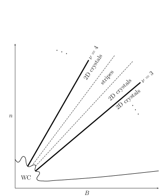
(a) 2DEG

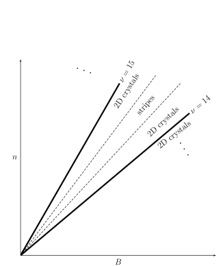
(b) graphene

Figure 1: Schematic phase diagrams for conventional 2DEG and graphene in the integer quantum Hall regime. Here $n$ is the electron density. “2D crystals” referred to in diagrams include bubble, quasiparticle and quasihole states, whose lattice constants are determined by the filling factor and magnetic length. These differ qualitatively from the Wigner crystal state where the lattice constant is set by the electron density. Fractional quantum Hall states, expected to appear at low filling factors in both diagrams, are not shown. The major difference between the two phase diagrams is that for the conventional 2DEG, the origin is completely surrounded by the Wigner crystal state, while in the graphene case, many different phases persist down to the origin.

The integer quantized Hall effect has been observed in graphene Novoselov et al. (2005); Zhang et al. (2005, 2006); Abanin et al. (2007), and, except for a well-understood shift in the precise values of the plateaus Ando (2005); Gusynin and Sharapov (2005), the Hall conductance appears rather similar to that found in the conventional 2DEG. Nevertheless, the behavior of clean and cold graphene in the low doping limit is likely to be different than that of the conventional 2DEG. Unlike the latter, non-interacting electrons in graphene to a good approximation obey a massless Dirac equation Ando (2005); Gusynin et al. (2007); Cas , with two inequivalent Dirac points in two different valleys (denoted as ${\bf K}$ and ${\bf K^{\prime}}$) in the Brillouin zone. When the system is undoped the Fermi energy passes directly through these Dirac points. With interactions, continuum Dahal et al. (2006) and tight-binding Dah studies of the this system in mean-field theory indicate that the system remains in a liquid state in zero magnetic field even at arbitrarily low doping. On the other hand, Hartree-Fock calculations Zhang and Joglekar (2007) and exact diagonalization studies Wan suggest that CDWs are possible in a large magnetic field – where states are restricted to a single or two Zha Landau levels (LLs) – and that the phase diagram is similar to that of the conventional 2DEG. In this paper we address the question of how the system passes from these strong-field states into the liquid state as the field and density are lowered to small values.

For the conventional 2DEG, the quantum Hall states give way to the WC in the low-field, low density limit due to Landau level mixing (LLM). This allows the electrons to form wavepackets that are more localized than is possible within a single Landau level, thereby lowering the interaction energy Zhu and Louie (1993). The degree of LLM is determined by a coupling constant $g$, the ratio of the typical Coulomb interaction energy $E_{C}$ to the scale of the LL separation. For both graphene and the conventional 2DEG, $E_{C}$ is given by $e^{2}/(\epsilon\ell)$, where $\ell=\sqrt{\hbar c/eB}$ is the magnetic length. However, the LL separations are different in the two cases. In the conventional 2DEG, it is given by $\hbar\omega_{c}=\hbar eB/mc$, so that $g\propto 1/\sqrt{B}$ and in the large $B$ limit where $g$ is small, LLM is negligible. In graphene, the LLs are not equally spaced Ando (2005), so we instead characterize it by the gap between the $n=0$ and $n=1$ LLs divided by $\sqrt{2}$, $\hbar v_{F}/\ell$, where $v_{F}$ is the Fermi velocity. Then $g=(e^{2}/\epsilon)/(\hbar v_{F})$ is a field-independent constant Dahal et al. (2006), typically estimated to be of order 1 or smaller. Nevertheless, even though $g$ is field-independent, the degree of LLM can change with $B$ even for fixed filling factor, and we shall see below that it in fact does, albeit by a small amount. This is because in addition to positive energy levels, the Dirac equation in a magnetic field supports negative energy Landau level states, as well as a zero energy LL, for each spin, provided the Zeeman energy is neglected. Moreover, the low energy theory of graphene involves two such Dirac points (${\bf K}$ and ${\bf K^{\prime}}$ valleys), so there are two copies of these energy levels in the spectrum. When undoped, all the negative energy states are filled, as well as one of the two zero-energy states Ando (2005). Added electrons interact with the electrons in these filled levels, which changes the effective energy of the higher LLs. Because the Landau level structure of these filled levels varies with field, the splitting between the $n=0$ and $n=1$ energy levels does not precisely the follow the $\sqrt{B}$ behavior discussed above.

In a continuum description, the filling of the negative levels is characterized by a (negative) integer $n_{c}$, which denotes the lowest LL which must be filled to accommodate one electron per atom, the density of mobile electrons of undoped graphene com ; Iyengar et al. (2007). An extra field dependence thus enters the problem through $n_{c}$, and is given by

$$-n_{c}=\frac{2S/(\sqrt{3}a^{2}/2)}{4S/2\pi\ell^{2}}\propto\frac{1}{B},$$ (1)

where $S$ is the area of the sample, $a=0.246\,\text{nm}$ is the lattice constant of the triangular (Bravais) lattice and the factor of 4 in the denominator comes from the spin and valley degeneracies. The interaction of electrons with those in the negative levels is most easily described in the Hartree-Fock (HF) approximation, where it appears as a contribution to the exchange self-energy. For uniform liquid states, we find that the Coulomb energy decreases faster with decreasing B than the difference in effective energy between the highest occupied level and the lowest unoccupied level, so that the ratio between kinetic and potential energy actually increases with decreasing $B$, because $|n_{c}|$ increases. We will demonstrate a similar effect for stripe states, and believe it should be ubiquitous for charge-ordered and liquid quantum Hall states.

Because this effect is a result of filling $|n_{c}|$ negative LLs, it is a concern that it may be an artifact of the cutoff procedure used in our HF calculations. To check this, we performed an analogous calculation for interacting electrons in a tight-binding model, where no artificial cutoff needs to be introduced. We obtain results from this model that are very similar to those of the continuum model.

The consequence of this is that, for states where LLM is small at large values of $B$, we expect it remain small, and even decrease, with decreasing $B$. While it is not immediately obvious that with $g\sim 1$ one should find weak LLM in these quantum Hall states, this does appear to be the case for WC and bubble states Zha , and as we demonstrate below, for stripe and uniform liquid states. The surprising result is that, within the Hartree-Fock approach, one expects these states to persist to arbitrarily small field. Thus, many different states persist down to the origin of the phase diagram in $n$ - $B$ plane [see Fig. 1(b)]. Because these states follow trajectories of fixed $\nu$ in the plane, the density of electrons participating these CDW states decreases with $B$, such that their amplitude scales roughly as $B$, and the wavelength as $1/\sqrt{B}$. The stripe states, and by analogy other CDW states, disappear continuously as $B\rightarrow 0$, eventually becoming indistinguishable from a uniform liquid state in the low field limit. Nevertheless, in principle, for a clean, undeformed graphene system, this implies that in principle many states emanate from the $B=n=0$ point in the phase diagram.

We note that this behavior is very specific to the $1/r$ form for Coulomb interactions that is natural in this system. For shorter range interactions, where a length scale other than the magnetic length is involved in the interaction range, the effective value of $g$ will increase with decreasing field as in the standard 2DEG, at low densities and fields LLM should destabilize the high field states, and a WC state should result. Such a situation could arise if a metallic gate is sufficiently close to the graphene plane to effectively screen the long-range component of the Coulomb interaction.

More generally, the behavior discussed here may be understood as being a consequence of the marginal nature of the $1/r$ Coulomb interaction in undoped graphene. As has been shown by us elsewhere Iyengar et al. (2007), the energy difference between Landau levels near the Fermi energy is increased by the filled Fermi sea, by an amount proportional to $\log|n_{c}|$. This logarithmic increase of the LL spacing with increasing $|n_{c}|$ can be reinterpreted as the Fermi velocity being renormalized upwards as the high-energy cutoff of the theory is increased Gonzalez et al. (1994). That the LL spacing increases slightly with increasing $|n_{c}|$ as the doping is decreased is consistent with interactions being marginally irrelevant in this system Gonzalez et al. (1994). Had it decreased instead, the interactions would be marginally relevant, one would expect to find a WC state near the origin of the $n-B$ phase diagram.

This paper is organized as follows. In Section II, we describe the continuum limit Hamiltonian, and the Hartree-Fock approximation used to study quantum Hall states in the presence of LLM. In Section III, we discuss the results of these continuum calculations. In Section IV, we introduce a tight-binding model with Hubbard interactions, and demonstrate that the suppression of LLM found in the continuum calculations is not an artifact of our cutoff procedure. Finally, we conclude with a summary in Section V.

II Hartree-Fock for Continuum Model

In standard 2DEG’s, it is known that the Hartree-Fock approximation is quite reliable for electronic states in high Landau levels Koulakov et al. (1996); Moessner and Chalker (1996). The situation should be similar for graphene, particularly if one can show that LLM is small for states in high LLs, as we will indeed find self-consistently below. We thus adopt the Hartree-Fock approximation for the states we study.

More specifically, our Hartree-Fock approach to the Dirac equation description of uniform and stripe quantum Hall phases in graphene is adapted from a procedure developed for electrons in a standard 2DEG Côté and MacDonald (1991); in what follows we briefly outline the method, and highlight the (largely technical) differences. The Hamiltonian for the system in a magnetic field is

$$\hat{H}=\sum_{1}\varepsilon_{1}\hat{c}_{1}^{\dagger}\hat{c}_{1}+\frac{1}{2}\sum_{1234}v_{1234}\hat{c}_{1}^{\dagger}\hat{c}_{2}^{\dagger}\hat{c}_{3}\hat{c}_{4},$$ (2)

where the numbers denote composite indices for the different quantum numbers specifying the states [e.g., $1\equiv(n_{1},\,X_{1},\,s_{1},\,t_{1})=$ (LL index, guiding center coordinate, spin, pseudospin (valley) index)],

$$\varepsilon_{1}=\varepsilon_{n_{1}}^{s_{1}}=\text{sgn}(n_{1})\frac{\hbar v_{F}}{\ell}\sqrt{2|n_{1}|}-s_{1}g^{\star}\mu_{B}B$$ (3)

is the LL spectrum plus the Zeeman energy, and

$$v_{1234}=\frac{1}{4}W_{1234}\delta_{s_{1}s_{4}}\delta_{t_{1}t_{4}}\delta_{s_{2}s_{3}}\delta_{t_{2}t_{3}}\prod_{i=1}^{4}(\sqrt{2})^{\delta_{n_{i},0}}$$ (4)

are matrix elements for the Coulomb interaction. $W_{1234}$ is related to standard matrix elements Côté and MacDonald (1991)

$$\tilde{V}_{n_{1},n_{2},n_{3},n_{4}} = \frac{1}{S}\sum_{\bm{q}}V(\bm{q})\left<n_{1},X_{1}|e^{i\bm{q}\cdot\bm{r}}|n_{4},X_{4}\right>$$

$$\times\left<n_{2},X_{2}|e^{-i\bm{q}\cdot\bm{r}}|n_{3},X_{3}\right>,$$

with $V(\bm{q})=2\pi e^{2}/q$ and

$$\left<n_{1},X_{1}|e^{i\bm{q}\cdot\bm{r}}|n_{4},X_{4}\right>$$

$$= \exp[i\frac{1}{2}q_{x}(X_{1}+X_{4})]F_{n_{1},n_{4}}(\bm{q})\delta_{X_{1},X_{4}+q_{y}\ell^{2}},$$

where

$$F_{n_{1},n_{4}}(\bm{q}) = \left(\frac{n_{4}!}{n_{1}!}\right)^{1/2}\left(\frac{(-q_{y}+iq_{x})\ell}{\sqrt{2}}\right)^{n_{1}-n_{4}}$$

$$\times\exp\left(\frac{-q^{2}\ell^{2}}{4}\right)L^{n_{1}-n_{4}}_{n_{4}}\left(\frac{q^{2}\ell^{2}}{2}\right)$$

for $n_{4}\leq n_{1}$, where $L^{\alpha}_{n}(x)$ is the generalized Laguerre polynomial. Note that $F_{n_{4},n_{1}}(\bm{q})=[F_{n_{1},n_{4}}(-\bm{q})]^{\ast}$.

In terms of $\tilde{V}$, $W$ takes the form

$$W_{1234} = (-i)^{|n_{1}|+|n_{2}|}i^{|n_{3}|+|n_{4}|}[\tilde{V}_{|n_{1}|,|n_{2}|,|n_{3}|,|n_{4}|}$$

$$+\text{sgn}(n_{1}n_{4})\tilde{V}_{|n_{1}|-1,|n_{2}|,|n_{3}|,|n_{4}|-1}$$

$$+\text{sgn}(n_{2}n_{3})\tilde{V}_{|n_{1}|,|n_{2}|-1,|n_{3}|-1,|n_{4}|}$$

$$+\text{sgn}(n_{1}n_{2}n_{3}n_{4})\tilde{V}_{|n_{1}|-1,|n_{2}|-1,|n_{3}|-1,|n_{4}|-1}].$$

Note that the guiding center coordinates ($X$) have been suppressed in the subscripts in Eqs. (II) and (II). The density matrix operators are defined as

$$\hat{\rho}^{nst}_{n^{\prime}s^{\prime}t^{\prime}}(\bm{q}) \equiv \frac{2\pi\ell^{2}}{S}\sum_{X}\exp(-iq_{x}X-\frac{1}{2}iq_{x}q_{y}\ell^{2})$$

$$\times\hat{c}^{\dagger}_{nXst}\hat{c}_{n^{\prime}\,X+q_{y}\ell^{2}\,s^{\prime}t^{\prime}}.$$

This relation may be inverted to obtain the expectation value of an arbitrary single-particle operator in terms of density operator expectation values,

$$\left<\hat{c}^{\dagger}_{nXst}\hat{c}_{n^{\prime}X^{\prime}s^{\prime}t^{\prime}}\right> = \sum_{\bm{p}}\left<\hat{\rho}^{nst}_{n^{\prime}s^{\prime}t^{\prime}}(\bm{p})\right>$$

$$\times\exp[\frac{1}{2}ip_{x}(X+X^{\prime})]\delta_{X,X^{\prime}-p_{y}\ell^{2}}.$$

For states with discrete translational symmetry, the sum over ${\bf p}$ is restricted to reciprocal lattice vectors $\left\{{\bf G}\right\}$. The interaction part of the HF Hamiltonian $\hat{H}_{HF}$ may now be written as

$$\hat{H}_{e-e}=\frac{S}{2\pi\ell^{2}}\sum_{n_{2},n_{3}}\sum_{\bm{G}}\sum_{s_{2},t_{2}}[U_{H}(n_{2},n_{3};\bm{G})\hat{\rho}^{n_{2}s_{2}t_{2}}_{n_{3}s_{2}t_{2}}(\bm{G})-\sum_{s_{1},t_{1}}U_{X}(s_{1},s_{2},t_{1},t_{2},n_{2},n_{3};\bm{G})\hat{\rho}^{n_{2}s_{2}t_{2}}_{n_{3}s_{1}t_{1}}(\bm{G})],$$ (9)

where

$$U_{H}(n_{2},n_{3};\bm{G}) \equiv \frac{e^{2}}{4\ell}\sum_{n_{1},n_{4}}\sum_{s_{1},t_{1}}H_{g}(n_{1},n_{2},n_{3},n_{4};\bm{G})\left<\hat{\rho}^{n_{1}s_{1}t_{1}}_{n_{4}s_{1}t_{1}}(-\bm{G})\right>,$$ (10)

$$U_{X}(s_{1},s_{2},t_{1},t_{2},n_{2},n_{3};\bm{G}) \equiv \frac{e^{2}}{4\ell}\sum_{n_{1},n_{4}}X_{g}(n_{1},n_{2},n_{3},n_{4};\bm{G})\left<\hat{\rho}^{n_{1}s_{1}t_{1}}_{n_{4}s_{2}t_{2}}(-\bm{G})\right>,$$ (11)

with

$$H_{g}(n_{1},n_{2},n_{3},n_{4};\bm{G})$$

$$\equiv (-i)^{|n_{1}|+|n_{2}|}i^{|n_{3}|+|n_{4}|}\prod_{i=1}^{4}(\sqrt{2})^{\delta_{n_{i},0}}[H(|n_{1}|,|n_{4}|,|n_{2}|,|n_{3}|;\bm{G})+\text{sgn}(n_{1}n_{4})H(|n_{1}|-1,|n_{4}|-1,|n_{2}|,|n_{3}|;\bm{G})$$

$$+\text{sgn}(n_{2}n_{3})H(|n_{1}|,|n_{4}|,|n_{2}|-1,|n_{3}|-1;\bm{G})+\text{sgn}(n_{1}n_{2}n_{3}n_{4})H(|n_{1}|-1,|n_{4}|-1,|n_{2}|-1,|n_{3}|-1;\bm{G})],$$

$$X_{g}(n_{1},n_{2},n_{3},n_{4};\bm{G})$$

$$\equiv (-i)^{|n_{1}|+|n_{2}|}i^{|n_{3}|+|n_{4}|}\prod_{i=1}^{4}(\sqrt{2})^{\delta_{n_{i},0}}[X(|n_{1}|,|n_{3}|,|n_{2}|,|n_{4}|;\bm{G})+\text{sgn}(n_{1}n_{3})X(|n_{1}|-1,|n_{3}|-1,|n_{2}|,|n_{4}|;\bm{G})$$

$$+\text{sgn}(n_{2}n_{4})X(|n_{1}|,|n_{3}|,|n_{2}|-1,|n_{4}|-1;\bm{G})+\text{sgn}(n_{1}n_{2}n_{3}n_{4})X(|n_{1}|-1,|n_{3}|-1,|n_{2}|-1,|n_{4}|-1;\bm{G})],$$

where

$$H(n_{1},n_{2},n_{3},n_{4};\bm{G})=\frac{1}{2\pi e^{2}\ell}V(\bm{G})F_{n_{1},n_{2}}(\bm{G})F_{n_{3},n_{4}}(-\bm{G}),$$ (12)

$$X(n_{1},n_{2},n_{3},n_{4};\bm{G})=\frac{\ell}{e^{2}S}\sum_{\bm{q}}V(\bm{q})F_{n_{1},n_{2}}(\bm{q})F_{n_{3},n_{4}}(-\bm{q})\exp(-i\bm{q}\times\bm{G}\ell^{2}).$$ (13)

The single-particle Green’s function is defined by

$$G^{nst}_{n^{\prime}s^{\prime}t^{\prime}}=-\left<T\hat{c}_{nXst}(\tau)\hat{c}^{\dagger}_{n^{\prime}X^{\prime}s^{\prime}t^{\prime}}(0)\right>,$$ (14)

and its Fourier-transform by

$$G^{nst}_{n^{\prime}s^{\prime}t^{\prime}}(\bm{G},\tau)=\frac{2\pi\ell^{2}}{S}\sum_{X}G^{nst}_{n^{\prime}s^{\prime}t^{\prime}}(X,X-G_{y}\ell^{2},\tau)\exp(-iG_{x}X+\frac{1}{2}G_{x}G_{y}\ell^{2}).$$ (15)

Within the HF approximation, the equation of motion (EOM) for $G^{nst}_{n^{\prime}s^{\prime}t^{\prime}}(\bm{G},\omega_{m})$ is given by

$$(i\omega_{m}+\mu/\hbar)G^{nst}_{n^{\prime}s^{\prime}t^{\prime}}(\bm{G},\omega_{m})-\frac{1}{\hbar}\sum_{t_{1},s_{1},n_{3},\bm{G^{\prime}}}A_{g}(s,t,n,s_{1},t_{1},n_{3};\bm{G},\bm{G^{\prime}})G^{n_{3}s_{1}t_{1}}_{n^{\prime}s^{\prime}t^{\prime}}(\bm{G^{\prime}},\omega_{m})=\delta_{nn^{\prime}}\delta_{ss^{\prime}}\delta_{tt^{\prime}}\delta_{\bm{G},0},$$ (16)

where

$$A_{g}(s,t,n,s_{1},t_{1},n_{3};\bm{G},\bm{G^{\prime}}) = \varepsilon^{s}_{n}\delta_{n_{3}n}\delta_{t_{1}t}\delta_{s_{1}s}\delta_{\bm{G^{\prime}}\bm{G}}$$

$$+[U_{H}(n,n_{3};\bm{G^{\prime}-G})\delta_{t_{1}t}\delta_{s_{1}s}-U_{X}(s_{1},s,t_{1},t,n,n_{3};\bm{G^{\prime}-G})]e^{i\bm{G}\times\bm{G^{\prime}}\ell^{2}/2}.$$

Because LLM could be important, we retain several “active” LLs (with LL indices between $n_{lower}$ and $n_{upper}$) around the chemical potential (see Fig. 2); i.e., we solve the EOM explicitly for the Green’s function matrix allowing off-diagonal elements in the LL index for values $n$ satisfying $n_{lower}\leq n\leq n_{upper}$. However, it would be incorrect to completely neglect the filled LLs below the active LLs ($n_{c}\leq n<n_{lower}$). These levels can enter the calculations through $U_{H}$ and $U_{X}$. However if sufficiently below the chemical potential, we expect LL mixing to be negligible for these states. We thus treat these levels as “inactive”, and fix their density matrix elements to be $\left<\hat{\rho}^{nst}_{n^{\prime}s^{\prime}t^{\prime}}(\bm{G})\right>=\delta_{nn^{\prime}}\delta_{ss^{\prime}}\delta_{tt^{\prime}}\delta_{\bm{G},0}$. (For self-consistency, we verify numerically that LL mixing for the lowest active level is very small, justifying the dividing point between active and inactive levels.) With this form the inactive levels do not contribute to $U_{H}$ due to the $(1-\delta_{\bm{G},0})$ in the Hartree term; i.e., it is precisely cancelled by an interaction with a uniform neutralizing background.Côté and MacDonald (1991) However, these levels do contribute a non-vanishing exchange energy $U_{X}$,

$$U_{X}^{inact}(s_{1},s_{2},t_{1},t_{2},n_{2},n_{3};\bm{G})=$$

$$\frac{e^{2}}{4\ell}\Sigma_{X}(n_{2},n_{3})\delta_{s_{1}s_{2}}\delta_{t_{1}t_{2}}\delta_{\bm{G},0},$$

where $inact$ stands for “inactive” and

$$\Sigma_{X}(n_{2},n_{3})=\sum_{n_{1}=n_{c}}^{n_{lower}-1}X_{g}(n_{1},n_{2},n_{3},n_{1};0).$$ (18)

We can rewrite Eq. (II) as

$$A_{g}(s,t,n,s_{1},t_{1},n_{3};\bm{G},\bm{G^{\prime}})$$

$$= [\varepsilon^{s}_{n}\delta_{n_{3}n}-\frac{e^{2}}{4\ell}\Sigma_{X}(n,n_{3})]\delta_{t_{1}t}\delta_{s_{1}s}\delta_{\bm{G^{\prime}}\bm{G}}$$

$$+[U_{H}^{act}(n,n_{3};\bm{G^{\prime}-G})\delta_{t_{1}t}\delta_{s_{1}s}$$

$$-U_{X}^{act}(s_{1},s,t_{1},t,n,n_{3};\bm{G^{\prime}-G})]e^{i\bm{G}\times\bm{G^{\prime}}\ell^{2}/2},$$

where the superscripts $act$ means now the summations in $U_{H}$ and $U_{X}$ are restricted to the active LLs.

\psfrag{m}{$\mu$}\psfrag{E}{$E$}\psfrag{act}{active}\psfrag{ina}{inactive}\psfrag{ngltd}{neglected}\psfrag{nc}{$n=n_{c}$}\psfrag{nn1}{$n=-1$}\psfrag{n0}{$n=0$}\psfrag{n1}{$n=1$}\psfrag{n2}{$n=2$}\psfrag{n3}{$n=3$}\psfrag{n4}{$n=4$}\psfrag{n5}{$n=5$}\psfrag{6}{$n=6$}\psfrag{7}{$n=7$}\includegraphics[scale={1.0}]{fig2}

Figure 2: Division of LLs into active and inactive LLs. In this example, $n_{lower}=1$ and $n_{upper}=5$. The upper and lower cutoffs of the active LLs are determined by the self-consistency conditions $1-\left<\hat{\rho}^{n_{lower}st}_{n_{lower}st}(0)\right>\,\ll 1$ and $\left<\hat{\rho}^{n_{upper}st}_{n_{upper}st}(0)\right>\,\ll 1$. Chemical potential $\mu$ for the case of filling $\nu=14$ is indicated as an example. In general several active levels are retained both above and below $\mu$ for all calculations reported here.

The calculations involve solving Eq. (16) to obtain the Green’s function, from which we obtain the density operator matrix elements. Finally, the Hartree-Fock energy is given by

$$E_{HF}$$

$$= \frac{S}{2\pi\ell^{2}}\sum_{{n_{2},n_{3}}\atop{(active)}}\sum_{s,t}\{[\varepsilon_{n_{2}}^{s}\delta_{n_{2}n_{3}}-\frac{e^{2}}{4\ell}\Sigma_{X}(n_{2},n_{3})]\left<\hat{\rho}^{n_{2}st}_{n_{3}st}(0)\right>$$

$$\quad+\frac{1}{2}\sum_{\bm{G}}[U_{H}^{act}(n_{2},n_{3};\bm{G})\left<\hat{\rho}^{n_{2}st}_{n_{3}st}(\bm{G})\right>$$

$$\quad-\sum_{s_{1},t_{1}}U_{X}^{act}(s_{1},s_{2},t_{1},t_{2},n_{2},n_{3};\bm{G})\left<\hat{\rho}^{n_{2}st}_{n_{3}s_{1}t_{1}}(\bm{G})\right>]\}$$

$$+\frac{S}{\pi\ell^{2}}\sum_{n\atop{(inact)}}[\sum_{s}\varepsilon_{n}^{s}-\frac{e^{2}}{4\ell}\Sigma_{X}(n,n)],$$

where the last line is a constant for given $B$ and $n_{lower}$.

III results of the continuum limit model

Table 1 details some typical results for the occupations of the various Landau levels near the Fermi energy. In this example $\nu=14.5$; i.e., the LL with $(nst)=(4\uparrow\Uparrow)$ is half-filled. Note that in this notation we denote the valley index as a pseudospin, with two values $\Uparrow$ and $\Downarrow$ denoting the ${\bf K}$ and ${\bf K^{\prime}}$ valleys respectively. We present results for different coupling constants in the range $0.5\lesssim g\leq 1$, consistent with previous estimates of its appropriate value Dah ; Iyengar et al. (2007). Our qualitative results are very similar for different values of $g$, even for (unphysical) values well above 1. We can see that the occupations immediately become very small above the half-filled LL, and very close to 1 below it, indicating that LLM is indeed small. This small level of mixing, in spite of the small non-interacting energy gap between LLs where the Fermi energy is located, may be understood as being a consequence of the large exchange enhancement of the gap due to the filled LLs. Furthermore, for smaller $B$, deviations of the occupations from a step function decreases (albeit just slightly), which means for decreasing field LLM becomes even less important. This unintuitive result occurs because of the large sea of negative energy LL states. With smaller field the degeneracy of each of these decreases, and so that more inert LLs need to be filled to obtain the correct density of electrons [see Eq. (1)]. In units of $e^{2}/\epsilon\ell$, the exchange interaction increases with increasing $|n_{c}|$, and the LLs effectively become slightly more separated.

Table 1: The diagonal density matrix elements $\left<\hat{\rho}^{nst}_{nst}(0)\right>$, indicating the occupation of the spin and pseudospin split LL with quantum numbers $(nst)$. The occupations are very close to a step function, indicating that LLM is weak. The deviation from a step function decreases as $B$ decreases, indicating that LLM becomes less important. Here $g$ is set to 1.

$n$	$st$	$\left<\hat{\rho}^{nst}_{nst}(0)\right>$
		$n_{c}=1872$	$n_{c}=12000$	$n_{c}=24000$
		($B=20T$)	($B=3.12T$)	($B=1.56T$)
$5$	$(\downarrow\Downarrow),(\downarrow\Uparrow),(\uparrow\Downarrow)$	$0.0000697757$	$0.000059254$	$0.0000559402$
$5$	$(\uparrow\Uparrow)$	$0.000520925$	$0.000425574$	$0.000396389$
$4$	$(\downarrow\Downarrow),(\downarrow\Uparrow),(\uparrow\Downarrow)$	$0.00078437$	$0.000651856$	$0.000611152$
$4$	$(\uparrow\Uparrow)$	$0.499997$	$0.50002$	$0.500026$
$3$	$(\downarrow\Downarrow),(\downarrow\Uparrow),(\uparrow\Downarrow)$	$0.999181$	$0.999318$	$0.999361$
$3$	$(\uparrow\Uparrow)$	$0.999567$	$0.999627$	$0.999647$

Fig. 3 illustrates the LLM for two integer fillings where the system is in a uniform liquid state. Here we measure the LLM by the quantity

$$M=\sum_{(nst)\neq(n^{\prime}s^{\prime}t^{\prime})}\left<\hat{\rho}^{nst}_{n^{\prime}s^{\prime}t^{\prime}}\right>^{2},$$

where the sum is over active LLs only ($n_{lower}=-5$ and $n_{upper}=5$). We again see that LLM is small and decreases as $B$ decreases for fixed filling factor.

Figure 3: LLM for integer fillings. Note $n_{c}\propto 1/B$, indicating the LLM decreases with decreasing field.

Previous studies of crystal and stripe states in graphene in which a single Dah ; Zhang and Joglekar (2007); Wan or small number Zha of Landau levels is retained find that such states can be stable in the presence of a magnetic field. Our study suggests that inclusion of the large number of LLs intrinsic to graphene not only does not change such results, but even increases their validity in weak fields. The result of this is that, within a zero-temperature mean-field description, one expects that in a very clean system many different states will persist down to the origin in a phase diagram plotted in the $n$ vs. $B$ plane [see Fig. 1(b))]. The state is determined only by the filling factor. This is in sharp contrast to the situation for conventional 2DEG’s, where LLM always destabilizes such states as the origin is approached.

One seeming paradox associated with this behavior is how the system approaches the uniform state which is believed, at least within a mean-field approach, to occupy the origin of the $n$ vs. $B$ phase diagram for graphene. The answer lies in noting that since LL mixing is negligible, the relevant length scale for the charge-ordered states of a partially filled LL is the magnetic length, which diverges as $B\rightarrow 0$. Fig. 4 illustrates the consequence of this for stripe states. One sees that the wavelength and amplitude of the density modulation are basically constants when measured in appropriate units ($\ell$ and $1/2\pi\ell^{2}$, respectively). Thus, these quantities should, up to logarithmic corrections, follow simple scaling relations,

$$\text{wavelength}\propto \ell \propto\frac{1}{\sqrt{B}},$$ (19)

$$\text{amplitude}\propto 1/\ell^{2} \propto B.$$ (20)

As $B$ decreases, the stripes, and we believe CDWs in general, “evaporate”, and thus approach the expected uniform density state at the origin.

Figure 4: Wavelength and amplitude for stripe with $\nu=14.5$, $n_{lower}=1$ and $n_{upper}=5$, as functions of the cutoff $n_{c}$ (and alternatively of the field $B$). The insets are density profiles for different $g$’s, with the arrows indicating the quantities plotted.

\psfrag{1}[cc]{1}\psfrag{2}[cc]{2}\psfrag{3}[cc]{3}\psfrag{4}[cl]{4}\psfrag{5}[cc]{5}\psfrag{6}[cc]{6}\psfrag{7}[cc]{7}\psfrag{8}[cl]{8}\psfrag{10}[cl]{$1^{\prime}$}\psfrag{20}[cl]{$2^{\prime}$}\psfrag{30}[cl]{$3^{\prime}$}\psfrag{40}[cl]{$4^{\prime}$}\psfrag{50}[cl]{$5^{\prime}$}\psfrag{60}[cl]{$6^{\prime}$}\psfrag{70}[cl]{$7^{\prime}$}\psfrag{80}[cl]{$8^{\prime}$}\psfrag{x}{x}\psfrag{y}{y}\includegraphics[scale={0.65}]{fig5}

Figure 5: Geometry of the tight binding problem. The unit cell corresponds to the area between the two armchair chains, including one of the bounding chains. In this example the unit cell contains 8 sites and 4 plaquettes. In our calculations, there are $n_{y}$ unit cells in the y direction, but only one in the x direction. We apply periodic boundary conditions to both x and y directions, so that site 8 is connected to site 1 by the bond to its right, etc..

IV hubbard model

The continuum limit forces one to adopt a cutoff in the occupied states, which in the previous section was accomplished by adopting an appropriate choice of the minimum occupied LL index, $n_{c}$. Since the increase of $n_{c}$ with decreasing field tends to suppress LLM, one may wish to consider whether a more physical cutoff scheme would give similar results. Towards this end we re-examine this question within a tight-binding Hubbard model. As in the continuum case, we look for states of this system within the Hartree-Fock approximation. For a simple on-site interaction $U$, the HF Hamiltonian for spin up electrons is

$$\hat{H}_{HF}(\uparrow)=\sum_{<ij>}t_{ij}\hat{a}^{\dagger}_{i\uparrow}\hat{a}_{j\uparrow}+U\sum_{i}\left<\hat{n}_{i\downarrow}\right>\hat{a}_{i\uparrow}^{\dagger}\hat{a}_{i\uparrow},$$ (21)

where $<ij>$ indicates nearest neighbors. For spin down electrons the Hamiltonian is analogous, with $\uparrow$ and $\downarrow$ interchanged.

We choose the unit cell to be the area between two adjacent armchair chains (see Fig. 5). We apply periodic boundary conditions to both x and y directions and study stripes oriented along the y directions. We can Fourier transform along the y direction, then we only need to define the phases of $t_{ij}$ along one armchair chain (e.g., the chain $12345678$ in Fig. 5), i.e., $t_{ij}\rightarrow t_{i,i+1}$, where $i=1,2,\ldots,n_{x}$ labels the sites in the unit cell ($n_{x}=8$ for the example in Fig. 5 and in general can be any integer multiple of 4). One possible choice is

$$\arg t_{i,i+1}=\left\{\begin{array}[]{l l}0&\quad\mbox{if $i$ is even}\\ (-1)^{(i-1)/2}(i-1)\pi\alpha&\quad\mbox{if $i$ is odd}\\ \end{array}\right.,$$

where $\alpha=2\Phi_{m}/n_{x}$ with $\Phi_{m}$ being the total number of flux quanta in the unit cell. (See Table 2.) Since $\Phi_{m}$ must be an integer, the magnetic fields for computationally tractable system sizes are actually very large compared to experiments. Nevertheless, we can deduce the qualitative behavior from these calculations.

Table 2: Nonzero $\arg t_{i,i+1}$ for hopping from site $i$ to $i+1$ on the chain $12345678$ in Fig. 5.

i	3	5	7
$\arg t_{i,i+1}$	$-2\pi\alpha$	$4\pi\alpha$	$-6\pi\alpha$

The coupling constant in this model is $g=U\ell/ta$, where $t\approx 2.7\,\text{eV}$ is the hopping amplitude of the tight-binding approximation. The situation that $g$ is field-independent does not arise naturally here; we introduce it by adjusting $U$ with field according to the relation

$$U\propto 1/\ell\propto\sqrt{B}\propto\sqrt{\frac{\Phi_{m}}{n_{x}}}.$$

For real Coulomb interactions, the effective HF potential includes a short-range exchange potential and a long-range Hartree potential, both proportional to $\sqrt{B}$. Stripe and bubble states result from the competition of these Koulakov et al. (1996); Moessner and Chalker (1996). Because of the highly local nature of the interaction in the Hubbard model, neither this scaling nor the effective long-range part of the interaction emerge: one only finds a local repulsion between electrons of different spins. Thus, the charge-ordered bubble and stripe states are not eigenstates of Eq. (21): one generically finds uniform density states. To obtain the former states, one needs to include longer-range interactions in the Hamiltonian. Obtaining full solutions of the HF approximation in this situation is possible but challenging, and is unnecessary for our more modest goal of testing the effect of using a real lattice rather than an energy cutoff. Thus, rather than fully solving for states of a system with long-range interactions, we include a slowly varying external potential which models the effect of the long range (non-contact) part of the potential. For simplicity we take this to have the form

$$\Delta\hat{H}(\uparrow)=A\sum_{i}\cos(2\pi x_{i}/L_{x})\hat{a}_{i\uparrow}^{\dagger}\hat{a}_{i\uparrow},$$

where $A$ must scale with field in the same way as $U$, and $L_{x}$ is the length of the unit cell along the x direction.

Figure 6: Stripe amplitude for Hubbard model calculation for a fixed ratio of unit cell width to magnetic length, as a function of $\Phi_{m}/n_{x}$, which is proportional to the field. $U/t=76.2\sqrt{\Phi_{m}/n_{x}}$, $A/U=0.1$. A straight line through the data points extrapolates rather accurately through the origin.

Our goal is to study how the density of a CDW state varies if the field is allowed to change, keeping the effective $g$ fixed. In order to make a fair comparison between states at different field strengths, we also fix the ratio $\frac{n_{x}}{\ell}\propto\sqrt{n_{x}\Phi_{m}}$ so that the width of the stripes and their spacing relative to the unit cell size does not change. This restricts the number of systems we can examine. However, the data we do get are in excellent agreement with the continuum model, i.e., the stripe amplitude (defined as the difference in maximum and minimum densities) is roughly proportional to the magnetic field (see Table 3 and Fig. 6). Note that in these calculations the amplitude decreases slightly faster than linearly with the field, consistent with a decreasing role for Landau level mixing. This effect is larger for larger values of $A/U$, as illustrated for example in Table 3.

Table 3: Change in stripe amplitude, defined as the difference between the maximum and minimum densities within a unit cell, when the magnetic field is changed by varying $\Phi_{m}$ and $n_{x}$. For first row of data, $A/U=0.2$; for second row, $A/U=0.15$. For all data, $U/t=76.2\sqrt{\Phi_{m}/n_{x}}$.

$(\Phi_{m},\,n_{x})$	$(\Phi_{m}^{\prime},\,n_{x}^{\prime})$	$B^{\prime}/B$	$\text{amplitude}^{\prime}/\text{amplitude}$
(1 , 600)	(2 , 300)	4	4.1941
(1 , 800)	(2 , 400)	4	4.1509

In Fig. 6 we illustrate the stripe amplitude for states generated for three values of $(\Phi_{m},\,n_{x})$, corresponding to three different magnetic fields, but with the ratios of the unit cell sizes and magnetic length the same, and with a relatively small value of $A/U$ (0.1). In this case one may fit a straight line through these points, and find that it extrapolates to the origin rather accurately. This is consistent with the stripe amplitude continuously vanishing in the $B\rightarrow 0$ limit, as was found in the continuum approach.

V summary

We have examined the stability of liquid and charge-ordered states for graphene (focusing on stripes as a paradigm for the latter) in the quantum Hall regime against the effects of Landau level mixing. Because the coupling constant $g$ is independent of field, we find the LLM does not increase with decreasing field, and that, counterintuitively, it decreases, albeit by a small amount. This latter effect is due to a large exchange enhancement of the LL gaps from the filled negative energy LLs, which increase in number as the field decreases. Within mean-field theory, this implies that clean and cold graphene at small fields and densities should support many different phases, determined solely by the filling factor. This contrasts with the conventional 2DEG, where a Wigner crystal state is believed to reside throughout this regime. In graphene, the liquid phase thought to exist in the absence of doping is reached in the $B\rightarrow 0$ limit at fixed filling factor by an “evaporation” of the CDW, in which the amplitude vanishes linearly with $B$.

- (1) See, e.g., A. H. Castro Neto and F. Guinea and N. M. R. Peres and K. S. Novoselov and A. K. Geim, cond-mat/0709.1163 (unpublished), and references therein.
- Fradkin and Kivelson (1999) E. Fradkin and S. A. Kivelson, Phys. Rev. B 59, 8065 (1999).
- Yi et al. (2000) H. M. Yi, H. A. Fertig, and R. Cote, Phys. Rev. Lett. 85, 4156 (2000).
- Cote et al. (2004) R. Cote, M. R. Li, H. A. Fertig, A. Faribault, and H. M. Yi, Int. J. Mod. Phys. B 18, 3527 (2004).
- Yi and Fertig (1998) H. M. Yi and H. A. Fertig, Phys. Rev. B 58, 4019 (1998).
- Mandal et al. (2003) S. S. Mandal, M. R. Peterson, and J. K. Jain, Phys. Rev. Lett. 90, 106403 (2003).
- Csathy et al. (2005) G. A. Csathy, H. Noh, D. C. Tsui, L. N. Pfeiffer, and K. W. West, Phys. Rev. Lett. 94, 226802 (2005).
- Novoselov et al. (2005) K. S. Novoselov, A. K. Geim, S. V. Morozov, D. Jiang, M. I. Katsnelson, I. V. Grigorieva, S. V. Dubonos, and A. A. Firsov, Nature 438, 197 (2005).
- Zhang et al. (2005) Y. B. Zhang, Y. W. Tan, H. L. Stormer, and P. Kim, Nature 438, 201 (2005).
- Zhang et al. (2006) Y. Zhang, Z. Jiang, J. P. Small, M. S. Purewal, Y. W. Tan, M. Fazlollahi, J. D. Chudow, J. A. Jaszczak, H. L. Stormer, and P. Kim, Phys. Rev. Lett. 96, 136806 (2006).
- Abanin et al. (2007) D. A. Abanin, K. S. Novoselov, U. Zeitler, P. A. Lee, A. K. Geim, and L. S. Levitov, Phys. Rev. Lett. 98, 196806 (2007).
- Ando (2005) T. Ando, J. Phys. Soc. Jpn. 74, 777 (2005).
- Gusynin and Sharapov (2005) V. P. Gusynin and S. G. Sharapov, Phys. Rev. Lett. 95, 146801 (2005).
- Gusynin et al. (2007) V. P. Gusynin, S. G. Sharapov, and J. Carbotte, Int. J. of Mod. Phys. B 21, 4611 (2007).
- (15) A.H. Castro Neto et al., cond-mat/0709.1163 (unpublished).
- Dahal et al. (2006) H. P. Dahal, Y. N. Joglekar, K. S. Bedell, and A. V. Balatsky, Phys. Rev. B 74, 233405 (2006).
- (17) H. P. Dahal and T. O. Wehling and K. S. Bedell and Jian-Xin Zhu and A. V. Balatsky, cond-mat/0706.1689 (unpublished).
- Zhang and Joglekar (2007) C.-H. Zhang and Y. N. Joglekar, Phys. Rev. B 75, 245414 (2007).
- (19) Hao Wang and D. N. Sheng and L. Sheng and F. D. M. Haldane, cond-mat/0708.0382 (unpublished).
- (20) C.-H. Zhang and Yogesh N. Joglekar, cond-mat/0802.4102 (unpublished) considered the influence of LLM on Wigner crystallization in graphene by retaining two Landau levels in the calculations. The sea of completely filled levels and the resulting effects of exchange with this sea on LLM were neglected. See discussion in text.
- Zhu and Louie (1993) X. Zhu and S. Louie, Phys. Rev. Lett. 70, 335 (1993).
- (22) We assume that the electrons in the negative levels can be described as filling an integral number of LLs. Although not precisely true, the discreteness of has little effect because in realistic situations is very large.
- Iyengar et al. (2007) A. Iyengar, J. Wang, H. A. Fertig, and L. Brey, Phys. Rev. B 75, 125430 (2007).
- Gonzalez et al. (1994) J. Gonzalez, F. Guinea, and M. A. H. Vozmediano, Nuc. Phys. B 424, 595 (1994).
- Koulakov et al. (1996) A. A. Koulakov, M. M. Fogler, and B. I. Shklovskii, Phys. Rev. Lett. 76, 499 (1996).
- Moessner and Chalker (1996) R. Moessner and J. T. Chalker, Phys. Rev. B 54, 5006 (1996).
- Côté and MacDonald (1991) R. Côté and A. H. MacDonald, Phys. Rev. B 44, 8759 (1991).