X-ray flares. Active late-type dwarfs

Abstract

We present temporal and spectral characteristics of X-ray flares observed from six late-type G-K active dwarfs (V368 Cep, XI Boo, IM Vir, V471 Tau, CC Eri and EP Eri) using data from observations with the XMM-Newton observatory. All the stars were found to be flaring frequently and altogether a total of seventeen flares were detected above the “quiescent” state X-ray emission which varied from 0.5 to 8.3 $\times 10^{29}$ $\rm{ergs}~{}\rm{s}^{-1}$. The largest flare was observed in a low activity dwarf XI Boo with a decay time of 10 ks and ratio of peak flare luminosity to “quiescent” state luminosity of 2. We have studied the spectral changes during the flares by using colour-colour diagram and by detailed spectral analysis during the temporal evolution of the flares. The exponential decay of the X-ray light curves, and time evolution of the plasma temperature and emission measure are similar to those observed in compact solar flares. We have derived the semiloop lengths of flares based on the hydrodynamic flare model. The size of the flaring loops is found to be less than the stellar radius. The hydrodynamic flare decay analysis indicates the presence of sustained heating during the decay of most flares.

1 Introduction

Flares are events in which a large amount of energy is released in a short interval of time. Such events take place at almost all frequencies of the electromagnetic spectrum and have been observed in the Sun as well as in many types of cool stars (Garcia-Alvarez, et al. 2002). These stellar flares could be radiating several orders of magnitude more energy than a solar flare. Optical flares in UV Cet (dMe) type stars are a common phenomenon. The flares produced by other stellar sources (e.g. RS CVn and BY Dra) are usually detected only in the UV or X-rays. These UV and X-ray flares show extreme luminosities and very hot temperatures ($\gtrsim 10$MK). Even though, flares in these stars present many analogies with the solar flares, there are also significant differences, such as the amount of energy released. A general model for stellar flares has emerged from numerous solar flare studies (Güdel 2004). The flare reconnection region, located somewhere at large coronal heights, primarily accelerates electrons and ions upto MeV energy (Dennis & Schwartz 1989). The accelerated electrons participate along the magnetic fields into chromosphere where they heat the cool plasma to coronal flare temperatures, thus evaporating a part of the chromosphere into the corona. Early X-ray observations with the EXOSAT observatory of flare stars revealed examples of two different type of flares: 1) Impulsive flares which are like compact solar flares, and 2) Long decay flares which are like two-ribbon solar flares (Pallavicini, Tagliaferri & Stella 1990). The compact flares are less energetic ($\sim$ 10³⁰ ergs s^-1), short in duration ($<1$ h), and confined to a single loop while the long-decay flares are more energetic ($\sim$ 10³² ergs s^-1), of long duration ($\geq 1$ h), and release the energy in an entire arcade of loops (Garcia-Alvarez 2000). The most likely flare process relates to an opening up of magnetic fields and subsequent relaxation by closing the open field lines.

Analysis of light curves during flares can provide us with insights into the characteristics of the coronal structures and, therefore, of the magnetic field (e.g., Schmitt & Favata 1999; Favata, Micela & Reale 2000a; Reale et al. 2004). Even though stellar flares are spatially unresolved, a great deal of information on the coronal heating and on the plasma structure morphology can be inferred from a detailed modeling of stellar flares; for instance, if sufficient data are available for moderately time-resolved spectral analysis, a study of the complete evolution of a flare can allow us to (a) infer whether the flare occurs in closed coronal structures (loops), (b) determine the size of the flaring structures, (c) determine whether continuous heating is present throughout the flare, and (d) put constraints on the location and distribution of the heating (see Reale et al. 2004).

Active solar-type (G-K) dwarfs are known to possess magnetic fields on their surfaces, and the field strengths are as large as several kilogauss, i.e. stronger than the strongest field observed on the Sun (e.g., Saar 1990; Johns-Krull & Valenti 1996). Cyclic behavior has been identified in several late-type active stars (Baliunas et al. 1995, Olah & Strassmeier 2002), suggesting that dynamos similar to the solar dynamos are also operative in solar-type stars. These solar-type stars are less active than the dMe stars (so called flare stars). However, they show more frequent flaring activity than the late-type evolved stars (e.g. RS CVns; Güdel 2004). In this paper, we present analysis of archival data obtained from XMM-Newton observations of six G-K dwarfs, namely V268 Cep, XI Boo, IM Vir, V471 Tau, EP Eri and CC Eri with the aim to understand the spectral and temporal characteristics of X-ray flares in them. In subsequent papers we will examine the characteristics of X-ray flares in the subgiants and the giants.

The paper is organized as follows: In §2 we give the basic parameters of stars in our sample, in §3 we describe the observational data sets that we have analysed and the methods of data reduction, §4 contains our analysis and results, and in §5 we present our discussion and conclusions.

2 Basic parameters of sample stars

The basic parameters of stars in our sample are given in Table 1. V368 Cep (= HD 220140; V = 7.54 mag) is a G9V spectral-type chromospherically active star with photometric period of 2.74 d (Chugainov, Lovkaya & Petrov 1991, Chugainov, Petrov & Lovkaya 1993). XI Boo (= HD 131156; V = 4.55 mag) is a nearby visual binary, comprising a primary G8 dwarf and a secondary K4 dwarf with an orbital period of 151 yrs (Hoffleit & Jaschek 1982). In terms of the outer atmospheric emission, UV and X-ray observations show that the primary dominates entirely over the secondary (Hartman et al. 1979, Ayres, Marstad & Linsky 1981, Schimtt 1997, Laming & Drake 1999). XI Boo A (primary) is a slow rotator with rotation period of 6.2 d (Gray et al. 1996). A cool main sequence eclipsing binary (G5V+KV), IM Vir (= HD 111487; V = 9.69 mag ) has an orbital period of 1.31d (Malkov et al. 2006). V471 Tau (= BD+16 516; V = 9.71) is a rapidly rotating detached eclipsing binary first observed by Nelson & Young (1970). The system is composed of a cool main-sequence chromospherically active K2 V star (Guinan & Sion 1984) and a degenerate hot white dwarf separated by 3.4 stellar radii. CC Eri (= HD 16157, V = 8.8) is a spectroscopic binary with orbital period of 1.561 d. It consists of a K7Ve primary and a dM4 secondary, with mass ratio of $\sim 2$ (Strassmeier et al. 1993). The primary star corotates with orbital motion due to the tidal lock, and is one of the fastest rotating K dwarfs in the solar neighborhood. EP Eri (=HD 17925, V = 6.0 mag) is very nearby (10.3 pc), very young (high Li I abundances), active K2-type dwarf with a rotation period of 6.85 days (Cayrel de Strobel & Cayrel 1989; Cutispoto 1992; Henry, Fekel & Hall 1995). The presence of an unresolved companion in this star has been suggested by Henry et al. (1995) based on the variable widths of the photospheric absorption lines reported in the literature ($v\sin{i}$ ranges from 3 to 8 km s^-1; see Fekel 1997).

3 Observations and Data Reduction

The late-type dwarf stars in our sample were observed with the XMM-Newton satellite using varying detector set-ups. The XMM-Newton satellite is composed of three co-aligned X-ray telescopes (Jansen et al. 2001) which observe a source simultaneously, accumulating photons in three CCD-based instruments: the twin MOS 1 and MOS 2 and the PN (Turner et al. 2001; Strüder et al. 2001), all three detectors constituting the EPIC (European Photon Imaging Camera) camera. The EPIC instrument consists of three CCD cameras with two different types of CCD, two MOS and one PN, providing the imaging and spectroscopy in the energy range from 0.15 to 15 keV with a good angular (PSF = 6 arcsec (FWHM)) and a moderate spectral resolution ($E/\Delta E\approx 20-50$). Exposure time for each star was in the range of 30-60 ks. A log of observations is provided in Table 2.

The data were reduced with standard XMM-Newton Science Analysis System (SAS) software, version 7.0 with updated calibration files (Ehle et al. 2004). The preliminary processing of raw EPIC Observation Data Files was done using the epchain and emchain tasks which allow calibration both in energy and astrometry of the events registered in each CCD chip and to combine them in a single data file for MOS and PN detectors. The background contribution is particularly relevant at high energies where coronal sources have very little flux and are often undetectable. Therefore, for further analysis we have selected the energy range between 0.3 to 10.0 keV. Event list file was extracted using the SAS task evselect. The epatplot task was used for checking the existence of pile-up affecting the inner region of all stars. Only the star CC Eri was found to be affected by pile-up. X-ray light curves and spectra of all target stars were generated from on-source counts obtained from circular regions with a radius $\sim$ 40-50^′′ around each source. However, for the star CC Eri, X-ray light curves and spectra were extracted with events taken from an annulus of 32^′′with inner radius of 12^′′to avoid pile-up effect in the inner region. The background was taken from several source free regions on the detectors at nearly the same offset as the source and surrounding the source.

4 Analysis and Results

4.1 Multi-band X-ray light curves and characterization of flares

The background subtracted X-ray light curves of six stars viz. V356 Cep, IM Vir, V471 Tau, CC Eri and EP Eri, as observed with the MOS and PN detectors are shown in Figures 1(a) to 1(f), respectively. All light curves are in the energy band 0.3-10.0 keV. The MOS and PN light curves are represented by solid and open circles, respectively. The temporal binning of light curves is 200 s for all sources. The PN light curve of the star IM Vir was affected by proton flares twice during the observations, first for 800 s after 10 ks from the beginning of the observation, and second at the end, after 40 ks of the observations. However, the MOS light curve was affected only at the end of the observation. For the star EP Eri, the high proton flare background region in the light curve is for a duration of 3 ks after 14.7 ks from the beginning of the observation. We have removed data during the proton flare background from the MOS and PN light curves of both the stars IM Vir and EP Eri. The star XI Boo was not observed by the PN detector, and only the light curve obtained with the MOS is presented here.

The light curves of all the individual stars show variability on a time scale of ks, most of which resembles flaring activity. The customary definition of a flare is a significant increase in intensity, after which the initial or quiescent level of intensity is reached again. Such patterns are observed in the light curves of the sample stars shown in Figures 1(a) to 1(f), and where the “flare regions” are represented by arrows and marked by Fi, where i=1,2…17 refers to the flare number. The mean quiescent level count rates of the sources are taken from regions that are free from flares and are marked by Q in the Figure 1. The start time, end time, flare duration and flux during quiescent and at flare peak for all the 17 flares observed are listed in Table 3. The peak and quiescent state count rates as given in Table 3 are converted into flux by using the WebPIMMS, where we assumed the plasma temperature of 1 keV. Flares F6, F7, F9, F14 and F16 were found to be long lasting ($\geq 2.3$ h) flares. Infact, the flare F7 of the XI Boo is longest flare observed with total duration of $\sim 3.1$ h. The peak flux in these long duration flares was found to be more than two times than the quiescent state. Other detected flares were shorter than 1.3 h. The shortest duration flare was detected one in V368 Cep (F3) and other in CC Eri (F12). In these short duration flares, peak X-ray flux was 1.3 - 1.8 times more than that of the quiescent state.

To characterize the flares, we have fitted the light curves of the flares with an exponential function

$$c(t)=A_{0}{\rm e}^{-\frac{t-t_{0}}{\tau_{d}}}+q$$ (1)

where c(t) is the count rate as a function of time t, t₀ is the time of peak count rate, q is the count rate in the quiescent state, $\tau_{d}$ is the decay time of the flare, and $A_{0}$ is the count rate at flare peak. The best fitted parameters for the flares are given in Table 4 for both the MOS and the PN data. Five flares, F6 and F7 of XI Boo, F9 of IM Vir, F14 of CC Eri and F16 of EP Eri the e-fold decay time was found to be more than 1 h. Flare F7 of XI Boo was found to be the longest decay flare ($\tau_{d}=10$ ks) observed among all the seventeen flares. The flare F16 shows a very different structure when compared to the other flares, i.e. a sharp rise and a highly structured decay as if more flares were present during the decay. Though it was tough to locate the peak of flare F16 because of its complex structure, the decay time was determined to be 4 ks. For the remaining eleven flares the decay time was found to be in the range of 8 - 47 minutes. The decay phase of the flare F17 was not observed. The rise times of all flares were found to be less than 1 h. The rise and decay time of the shortest flare F3 of V368 Cep was found to be 0.5 ks. In XI Boo, after the flare F6 an active level U was identified, where average flux was 1.8 times more than that of the Q state (see Figure 1(b)), that was higher than the peak of the flare F5 indicating a very high activity level. Two similar highly active regions U1 and U2 were identified between the flares F13 and F14. The average fluxes during the regions U1 and U2 were 1.3 and 1.4 times more than that of the quiescent state. Presence of strong substructures in these active regions indicates superposition of a large number of flaring regions.

To investigate the behavior of the flares detected in different energy bands, the light curves of the stars obtained with the MOS and PN are divided into three energy bands namely soft (0.3 - 0.8 keV), medium (0.8 - 1.6 keV), and hard (1.6 - 10 keV). The boundaries of the selected energy bands are chosen as the line free regions of the low resolution PN spectra. The hardness ratio HR1 and HR2 are defined by the ratio of medium to soft band, and hard to medium band count rate, respectively. The soft, medium, hard band intensity curves, and the hardness ratio curves HR1 and HR2 as a function of time are shown in the sub-panels running from top to bottom in left(MOS) and right(PN) of Figure 2 (a) for the star V368 Cep. Similar plots of intensity and hardness ratios observed from the stars XI Boo, IM Vir, V471 Tau, CC Eri and EP Eri are shown in the Figures 2(b) to 2(f), respectively. The light curves in individual band also show significant variability in all sources. We have determined the e-folding decay time of observed flares in the three bands by fitting equation (1). The decay times, rise times, count rates at flare peaks, and quiescent state count rates at soft, medium and hard band for PN data are given in the Table 5. For most of the flares, e-folding decay time in the soft band was found to be more than the decay time in the medium and the hard band. However, for the flare F3 of V368 Cep and F7 of XI Boo, it appears that decay time in the medium band was more than in the soft band. For the flares F6, F7 and F9 the decay time in the soft band was found to be more than 3.0 ks than that of the hard band. However, for other flare events the decay time in the soft band was $\lesssim 2$ ks than that in the hard band. Two smaller flare like structures were seen just after the peak of flare F13 of CC Eri, in the hard band but were not observed in the soft and medium band light curves (see Figure 2(e)). The rise time for all flares in all band was found to be well within $1\sigma$ level (Table 5).

The flare peak to the quiescent state flux ratio in the hard band was found in between 2-16, which is more than that of the similar ratios in the medium and the soft band (see also Table 5) for all flares. In terms of the peak flux, the flares F6 and F7 of XI Boo, and F13 and F14 of CC Eri were stronger in the medium band than in the soft and the hard band. The variation in the hardness ratio are indicative of changes in coronal temperature. An X-ray flare is well defined by a rise in the temperature and subsequent decay. For the flares F6, F7, F9, F12, F13 and F14, both HR1 and HR2 varied in the similar fashion to their light curves (see Figure 2). This implies that an increase in the temperature at flare peak and subsequent cooling. The structures observed during the decay phase of the flares F2 of V368 Cep and F13 of CC Eri in the hard band were also observed in the HR2 curve. This could probably be due to emergence of flares during the decay phase of these flares, which were comparatively stronger in the hard band. During the flares F2, F3 and F4 of V368 Cep, and F16 of EP Eri the HR1 did not show any variation but HR2 varied according to the flare intensity. However, HR1 and HR2 did not show any significant variation during the flares F1, F5, F8, F10, F11, F15 and F17. The PN data have more count rates than the MOS and have similar characteristics to that of MOS, therefore, for further analysis in this paper we use only the PN data.

4.2 Colour-colour diagrams

Plots of hardness ratio in the form of colour-colour (CC) diagram can reveal information about spectral variations and serve as a guide for a more detailed spectral analysis. For this purpose, the light curves and the hardness ratio curves of the flares were divided into different time segments covering their rising and decaying phases as shown in Figure 1, where Ri(i=1,2..) represents the rising phase, Di(i=1,2,..) represents the decay phase and Q represents the quiescent state. We determined the HR1 and HR2 from the PN data for each of these segments and plotted the values in Figure 3. To understand the observed behavior of HR1 and HR2 in terms of simple spectral models, we generated the soft(0.3-0.8 keV), medium(0.8-1.6 keV) and hard(1.6-10.0 keV) band count rate using the “fakeit” provision in the XSPEC, using the most recent Canned Response Matrices downloaded from http://xmm.vilspa.esa.es/external/xmm_SW_cal/calib/epic_files.html, and simple two temperature plasma models. The two temperature APEC models were mixed such that the emission measure were in the ratio $EM_{2}/EM_{1}$ of 0.4, 0.6, 0.8, 1.0 and 1.2 (based on spectral results in §4.3 and §4.4). The abundances (0.25) and hydrogen column density ($10^{20}$ cm^-2) were kept fixed for each set of the $EM_{2}$/$EM_{1}$ (see §4.3 and §4.4). Further by keeping $kT_{1}$ fixed at different values ranging from 0.2 to 1.2 keV in steps of 0.2 and varying $kT_{2}$ from 0.4 to 2.4 keV such that $kT_{2}>kT_{1}$, we generated count rates in the soft, medium and hard bands. These predicted count rates were used to generate the hardness ratios. The families of curve thus generated are over-plotted on the data points in Figure 3 to understand the CC diagram. The kT₂ in Figure 3 increases from bottom to top of each curve.

Figure 3 (a) shows the plot between HR1 and HR2 for a set of $EM_{2}$/$EM_{1}$ = 1.0 for the star V368 Cep. In the case of the flare F1, ’D1’ intersects the generated CC curves for which $kT_{1}$ is 0.6 keV, however, ’D4’ intersects the curve generated for $kT_{1}~{}=$ 0.2 keV. A similar pattern is seen for the other flares F2 and F4 of the stars V368 Cep, where the top of the flare is located near the CC curve for a high temperature component whereas the colours near the end of the flare intersect the CC curve corresponding to a lower temperature. The flare F2 shows a very high temperature during its rise phase ’R1’ and the decay phase ’D5’, as both are located between the CC curves of 1.0 and 1.2 keV. The decay phase D6 of the flare F2 is located near the 0.8 keV CC curve. The peak seen during the decay phase D6 of flare F2 (Fig 3(a)) can be explained by a rise in the temperature of coronal plasma. It appears that the quiescent state ’Q’ of the star V368 Cep has a cool temperature between 0.2 to 0.4 keV.

The peak of the largest flare ’F9’ observed in the star IM Vir appears to have a temperature between 1.0 - 1.2 keV. As the flare decayed the temperature was also observed to decrease. A similar trend is seen during the flares observed in the stars XI Boo (Figure 3(b)), V471 Tau (Figure 3(d)), CC Eri (Figure 3(e)), and EP Eri (Figure 3(f)). The observed CC curves for the star IM Vir, V471 Tau and CC Eri were well matched with the generated family of CC curves for a set of $EM_{1}/EM_{2}$ = 1.0. However, the observed CC diagram of EP Eri were well matched with generated CC curves for a set of $EM_{1}/EM_{2}=0.4$. It appears that high temperatures are needed during the flare peak, and the plasma temperatures decrease as flare decays. To, further confirm and quantify the spectral changes during the flare, we have also performed a detailed spectral analysis of the flares and the quiescent states of the stars. The results of these analyses are presented below.

4.3 Quiescent state X-ray spectra

X-ray spectra for each star during the quiescent state were analysed using XSPEC version 12.3 (Arnaud 1996). Data were cleaned of proton flares by removing the affected time periods for the stars IM Vir and EP Eri. Spectral analysis of EPIC data was performed in the energy band between 0.3-10.0 keV for the star V368 Cep, XI Boo, V471 Tau and CC Eri, while for the stars IM Vir and EP Eri spectral analysis was performed between 0.3-5.1 keV. Individual spectra were binned so as to have a minimum of 20 counts per energy bin. The EPIC spectra of the stars were fitted with a single (1T) and two (2T) temperature collisional plasma model known as APEC (Astrophysical Plasma Emission Code, Smith et al. 2001), with variable elemental abundances. Abundances for all the elements in the APEC were varied together. The interstellar hydrogen column density ($N_{H}$) was left free to vary. For all the stars, no 1T or 2T plasma models with solar photospheric (Anders & Grevesse 1989) abundances could fit the data, as unacceptably large values of $\chi^{2}_{\nu}$ were obtained. Acceptable APEC 2T fits were achieved only when the abundances were allowed to depart from the solar values. The best-fit 2T plasma models with sub-solar abundances along with the significance of the residuals in terms of $\Delta\chi^{2}$ are shown in Figures 4(a) to (f) for all the stars. Table 6 summarizes the best-fit values obtained for the various parameters along with the minimum $\chi_{\nu}^{2}=\chi^{2}/\nu$ (where $\nu$ is degrees of freedom) and the 90% confidence error bars estimated from the minimum $\chi^{2}+2.71$. The derived values $N_{H}$ from the spectral analysis were found to be lower than that of the total galactic HI column density (Dicky & Lockman 1990) towards the direction of that star. The cool and hot temperatures at the quiescent state of these stars were found in the range of 0.2 - 0.5 and 0.6 - 1.0 keV, respectively. The corresponding EM2/EM1 during the quiescent state of each star was found in the range of 0.8 - 1.2, except for the star EP Eri where it was found to be $\sim 0.4$.

4.4 Spectral evolution of X-ray flares

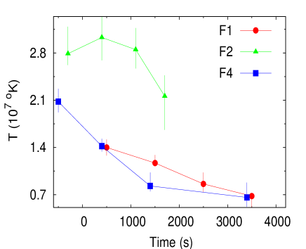
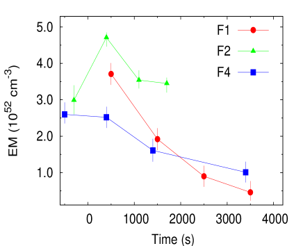
Figure 5: Plots of (a) temperature and (b) emission measure during the flares F1, flare F2, and F4 of the star V368 Cep. Here, ’0’ time corresponds to flare peak and negative scale of time indicates the flare during its rise phase.

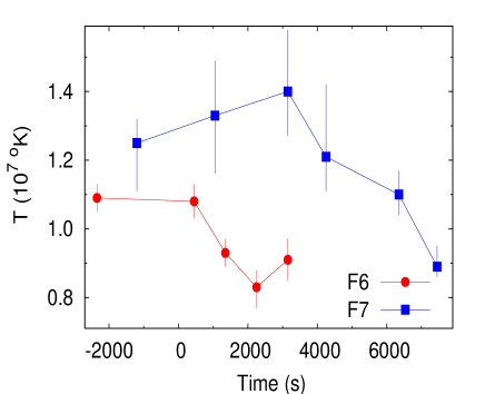
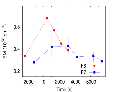
Figure 6: Plots of (a) temperature and (b) emission measure of dominant component of 2T fit during the flares F6 and F7 of the star XI Boo.

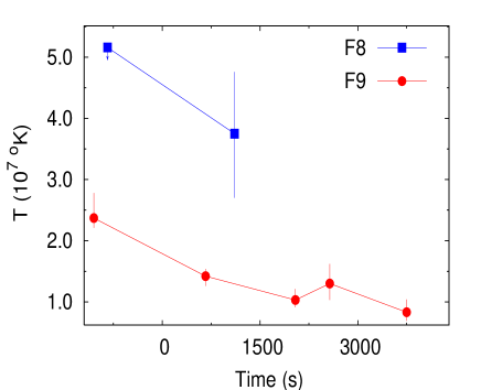
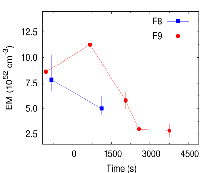
Figure 7: Plots of (a) temperature and (b) emission measure during the flares F8 and F9 of the star IM Vir. Here arrow shows upper limit on data point.

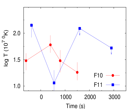
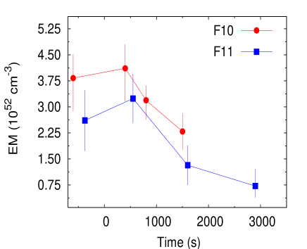
Figure 8: Plots of (a) temperature and (b) emission measure during the flares F10 and F11 of the star V471 Tau. Here, arrow shows the upper limit on data point.

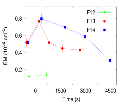
Figure 9: Plots of (a) temperature and (b) emission measure during the flares F12, F13 and F14 of the star CC Eri. Here, arrow shows lower limit on the data point

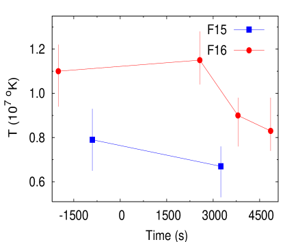
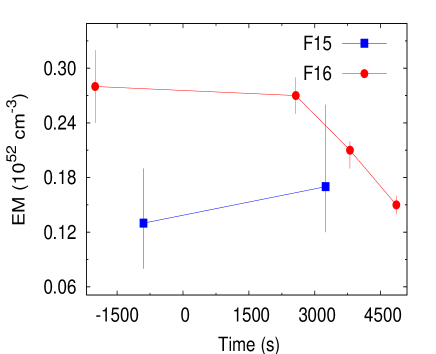
Figure 10: Plots of (a) temperature and (b) emission measures during the flares F15 and F16 of the star EP Eri.

In order to trace the spectral changes during the flares, we have analysed the spectra of the different time intervals shown in Figure 1. To study the flare emission only, we have performed 1-T spectral fits of the data, with the quiescent emission taken into account by including its best-fit 2-T model as a frozen background contribution. This is equivalent to consider the flare emission subtracted of the quiescent level, allows us to derive one “effective” temperature and one emission measure of the flaring plasma. The abundances were kept fix to that of the quiescent emission. The best fit spectral parameters for each flare segments are listed in Table 7. Figures 5 - 10 show the temporal evolution of the temperature and corresponding emission measure of the flares detected in the targeted stars, where ’0’ time corresponds to the flare peak time.

4.4.1 V368 Cep

Spectral data of flares F1, F2 and F4 were binned into four segments. However, for the flare F3 data could be collected over only one segment. Both the temperature and the corresponding emission measure were found to decrease from the flare peak to the quiescent state (see also Table 7). As shown in Figure 5(a), the highest temperature for the flare F1 was 14 MK and decreased along the decay path to 6.8 MK. A similar trend was also found in the emission measure, where it increased by a factor of seven (see Figure 5 (b)). The temperature and emission measure for the flare F2 were peaked simultaneously during the decay phase D5. However, for the flare F4 both parameters were peaked during the rise phase R2. The maximum luminosity was found during the flares F2 and peaked at $1.18\times 10^{30}$ $\rm{ergs}~{}\rm{s}^{-1}$, which is $\sim 1.7$ times more than that of the quiescent state.

4.4.2 XI Boo

To see the flare evolution, flare F6 and F7 have binned into five and six intervals, respectively. For the flare segments R2, D5, D6, D7 and D8, the 1T APEC fit gave high value of $\chi^{2}_{\nu}$ (=1.5 for R2, 1.75 for D5, 1.61 for D6, 1.55 for D7 and 1.34 for D8). The spectral fit to the data for these time segments improves the $\chi^{2}$ by using the 2T plasma model (see Table 7). The temperature and the corresponding emission measure of the cool component for these time segments were found to be constant at $0.6\pm 0.1$ keV and $4.0\pm 1.0\times 10^{51}$ cm^-3, respectively. The spectral parameters for hot component of the best fit 2T plasma model are reported in Table 7. The evolution of the temperature of hot component and the corresponding emission measure are shown in Figures 6 (a) and 6 (b), respectively. For the flares F6 and F7, both the temperature and corresponding emission measure were reached to the maximum value during the decay phase. As mentioned in Table 6 and 7, during the flares F6 and F7, XI Boo was $\sim 2$ times more X-ray luminous than that of the quiescent state.

4.4.3 IM Vir

The spectral data of the flares F8 and F9 were binned in two and four different time segments, respectively (see Figure 1(c)) and spectra of each segment were fitted with 1T APEC model. The plots of temperature and the corresponding emission measure are shown in Figures 7 (a), and (b), respectively. For the flare F9, the maximum fit temperature, was reached during the rising phase R2, somewhat earlier than the maximum of its emission measure. The emission measure was increased by a factor of four during the flare F9. The luminosity at the peak of flare F9 was found to be $\sim 2$ times more than that of the quiescent state.

4.4.4 V471 Tau

Two flares detected in the star V471 Tau were examined by analysing four different time intervals during the flares. Figures. 8 (a) and (b) show the plot of temperature and the corresponding emission measure during the flares F10 and F11. For the flare F10 the temperature reached its maximum value of $17.8$ MK and decreased along the decay phase (see Table 7). The corresponding emission measure was also peaked during the decay phase of the flare F10 (see Figure 8(b) and Table 7). For the flare F11, both the temperature and the emission measure follow similar trend to the flare light curve. The X-ray luminosity was increased by a factor of $\sim 1.6$ for the flare F10 and $\sim 1.4$ for the flare F11.

4.4.5 CC Eri

The evolution of temperature and the corresponding emission measure for three flares F12, F13 and F14 are shown in Figures 9 (a) and (b), respectively. Small variations were found in the temperature and the emission measure during the flares F13 and F14. Both the temperatures and the corresponding emission measures were found to decrease during the decay phase for all flares (see also Table 7). The temperature and the corresponding emission measure for all the flares were peaked during the decay phase. However, it appears that temperature is peaked before the emission measure for the flare F13. The peak luminosity during flares F13 and F14 was found to be $6.0\times 10^{28}$ $\rm{ergs}~{}\rm{s}^{-1}$ more than that of the quiescent state.

4.4.6 EP Eri

Spectra of different time segments of the flares are fitted with 1T plasma models. Figures 10 (a) and (b) show the evolution of temperature and the corresponding emission measure for the flares F15 and F16. For the flare F16, both the temperature and the corresponding emission measure were peaked during the rise phase R2, remained constant upto the decay phase D2 and then decreased along the flare decay without any appreciable changes in the luminosity. The luminosity during both flares was found to be similar to that of the quiescent state (see Table 6 and Table 7).

4.5 Loop modeling of the X-ray flares

Flares can not be resolved spatially on a star. However, by an analogy with solar flares and using flare loop models, it is possible to infer the physical size and morphology of the loop structures involved in a stellar flare. The most widely used but approximate methods for analyzing stellar flares are: i) Two-ribbon flare method (Kopp & Poletto 1984), ii) Quasi-Static Cooling method (van den Oord & Mewe 1989), iii) Pure radiation cooling method (Pallavicini et al. 1990), iv) Rise and decay time method (Hawley et al. 1995), and v) Hydrodynamic method (Reale et al. 1997). The Two-ribbon flare model assumes that the flare decay is entirely driven by heating released by magnetic reconnection of higher and higher loops and neglects completely the effect of plasma cooling. The other four methods are instead based on the cooling of plasma confined in a single flaring loop. In the hypothesis of flares occurring inside closed coronal structures, the decay time of the X-ray emission roughly scales as the plasma cooling time. In turn, the cooling time scales with the length of the structure which confines the plasma: the longer the decay, the larger is the structure (e.g. Haisch et al.1983). A loop thermodynamic decay time has been derived (van den Oord & Mewe 1989; Serio et al. 1991) as:

$$\tau_{th}=\frac{120L_{9}}{\sqrt{T_{7}}}$$ (2)

where $L_{9}$ and $T_{7}$ are the loop half-length and the maximum temperature (T_max) of the flaring plasma, in units of $10^{9}$ cm and $10^{7}$ K, respectively. The timescale above is derived under the hypothesis of impulsive heat released at the beginning of a flare.

The hydrodynamic model includes both plasma cooling and the effect of heating during flare decay. Reale et al. (1997) presented a method to infer the geometrical size and other relevant physical parameters of the flaring loops, based on the decay time and on evolution of temperature and the emission measure (EM) during the flare decay. The empirical formula for the estimation of the unresolved flaring loop length has been derived as:

$$L_{9}=\frac{\tau_{d}\sqrt{T_{7}}}{120f(\zeta)}~{}~{}~{}~{}~{}~{}~{}~{}f(\zeta)\geq 1$$ (3)

where $\tau_{d}$ is the decay time of the light curve, and $f(\zeta)$ is a non-dimensional correction factor larger than one. $\zeta$ is the slope of the decay path in the density-temperature diagram (Sylwester et al. 1993) and is maximum ($\sim 2$) if heating is negligible and minimum ($\sim 0.5$) if heating dominates the decay. The correction factor $f(\zeta)$ and loop maximum temperature are calibrated for the XMM-Newton EPIC spectral response and are given as (Reale 2007):

$$f(\zeta)=\frac{0.51}{\zeta-0.35}+1.36~{}~{}~{}~{}~{}~{}~{}~{}~{}~{}~{}\rm{(for~{}0.35<\zeta\leq 1.6)}$$ (4)

$$T_{max}=0.13T_{obs}^{1.16}$$ (5)

Other physical properties of the flaring plasma can be inferred from the analysis of flare data. The analysis of X-ray spectra provides values of the temperature and emission measure. From the emission measure (EM) and the plasma density ($n_{e}$), the volume of the flaring loop is estimated as (Reale 2002):

$$V=\frac{EM}{n^{2}_{e}}$$ (6)

where V is the loop volume. It has been shown that in the equilibrium condition the loop scaling laws hold, linking maximum pressure, temperature, loop length and heating rate per unit volume as (Rosner, Tucker & Vaiana 1978, Kuin & Martens 1982):

$$T_{max}=1.4\times 10^{3}(pL)^{1/3}$$ (7)

$$E_{H}\approx 10^{-6}T_{max}^{3.5}L^{-2}~{}~{}~{}ergs~{}s^{-1}cm^{-3}$$ (8)

The minimum magnetic field necessary to confine the flaring plasma can be simply estimated as

$$B=\sqrt{8\pi p}$$ (9)

Because of limited statistics, we have modeled only ten flares. The results of the model parameters are listed in Table 8. In this table, column 1 is name of the star and the corresponding flare, column 2 is slope of density-temperature diagram ($\zeta$), column 3 contains loop maximum temperature based on spectral fit and equation (5), semiloop length is determined using the equation (3) and given in column 4, pressure in the loop at the flare peak is estimated using the loop scaling law (see equation (7); column 5), column 6 contains maximum electron density at the flare loop (we have assumed a totally ionized hydrogen plasma i.e. $p=2n_{e}kT_{max}$; since pressure derived from equation (7) is a maximum value, therefore, a upper limit on density is estimated), volume of the flaring plasma is estimated from maximum emission measure and from the estimated maximum electron density, and therefore, is treated as lower limit (equation (6); column 7), column 8 is heating rate per unit volume and estimated using equation (8), the minimum magnetic filed necessary to confine the flaring plasma at loop apex $B$ (see equation 9) is given in column 9, the loop aspect ratio $\beta$ (=$r/L$, $r$ is radius of the loop cross section, assuming circular) estimated from the loop scaling law $V=2\pi\beta^{2}L^{3}$ and number of loops filling the flare volume estimated assuming that $\beta=0.1$ for a single loop are given in column 9 and 10, respectively. The model parameters for the different flares from each star are presented and discussed below.

4.5.1 Flares F1, F2 and F4 of V368 Cep

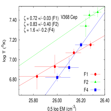
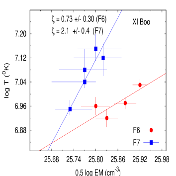
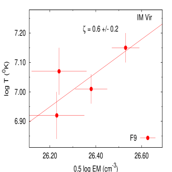
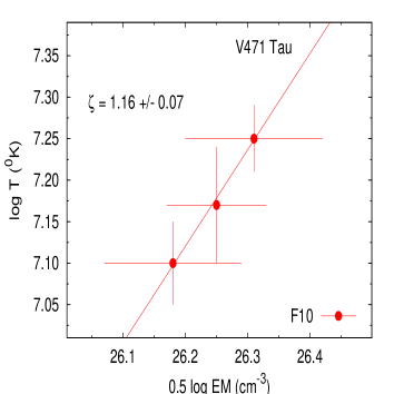
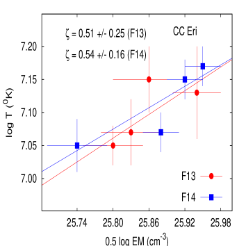
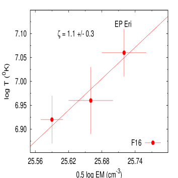
Figure 11: The density-temperature diagram, where EM^1/2 has been used as a proxy of density. Symbols for the each flares are given at the bottom right corner. Straight lines represent the best linear fit to the corresponding data. $\zeta$ is slope of density-temperature diagram.

The average temperatures of the loops, usually lower than the real loop maximum temperatures, are found from the spectral analysis of the data as given in §4.4. According to equation (5), the loop maximum temperatures for the flare F1, F2 and F4 are found to be $25.5\pm 2.5$, $62\pm 8$ and $40.3\pm 1.8$ MK, respectively. Figure 11 (a) shows the density-temperature (n-T) diagram, where EM^1/2 has been used as a proxy of density. In Figure 11 (a) the flares F1 ,F2 and F4 are represented by solid circles , solid triangles and solid squares, respectively. The solid lines represent the best linear fit to the corresponding data, providing the slope $\zeta$. These values of $\zeta$ indicate the presence of a sustained heating during the decay of the flares F1 and F2. However, sustained heating is negligible during the decay of the flare F4. As discussed in §4.5, the e-folding time of the light curve and the slope of n-T path can be used to estimate the loop half-length. According to equation (3) the semiloop lengths for the flares F1, F2 and F4 are determined to be $6.0\pm 0.6\times 10^{9}~{}(=0.1R_{\star})$, $19.8\pm 8.6~{}(=0.4R_{\star})$ and $11.7\pm 1.3\times 10^{9}~{}(=0.2R_{\star})$ cm, respectively. These loop lengths are much smaller than the pressure scale height $h_{p}>1.2\times 10^{11}$ cm. Maximum pressure in the loop at the flare peak is estimated to be $>10^{3}$ dyne cm^-2 for the flares F1, F2 and F4, respectively (see equation (7)). Assuming that the hydrogen plasma is totally ionized ($p=2n_{e}kT_{max}$), the maximum plasma density in the loop at the flare peak is estimated in the order of $10^{11}$ cm^-3 for the flares F1, F2 and F4, respectively. We computed a volume of $\sim 1.78\times 10^{30}$ cm^-3 for the flare F1 using the observed peak EM of $3.7\times 10^{52}$ cm^-3. Similarly, loop volume is determined to be $7.2\times 10^{29}$ cm³ for flare F2 and $7.4\times 10^{29}$ cm³ for the flare F4. A hint for the heat pulse intensity comes from the flare maximum temperature. By applying the loop scaling laws and loop maximum temperature (see equation (8)) the heat pulse intensity for the flares F1, F2 and F4 would be the order of 2.36, 4.75 and 3.06 ergs cm^-3 s^-1, respectively. From the pressure of the flare plasma the magnetic field required to confine the plasma should be more than the 160 Gauss for all the flares.

4.5.2 Flares F6 and F7 of XI Boo

The evolution of flare F6 and F7 in n - T plane is shown in Figure 11 (b), together with a least square fit to the decay phase. The resulting best-fit slopes ($\zeta$) for the decaying phase of flare F6 and F7 indicate that the flare F6 is driven by the time scale of the heating process, whereas sustained heating is negligible during the decay of the flare F7. The intrinsic flare peak temperatures for flare F6 and F7 are, applying equation (5) to the observed maximum temperature , $18.9\pm 0.8$ and $25.3\pm 2.7$ MK, respectively. For the flare F6 the semiloop length is estimated to be less than the pressure scale height, $h_{p}=10^{11}$ cm. Maximum pressure and density in the loop at the peak of the flare F6 are estimated to be $130\pm 6$ dyne cm^-2 and $2.5\pm 1.0\times 10^{10}$ cm^-3, respectively. Using equation 6, volume of the flaring plasma is estimated to be $1.1\times 10^{31}$ cm³. A minimum magnetic field of $\sim 58$ Gauss is required to confine the flaring plasma at the peak of the flare. Although, the value of $\zeta$ for the flare F7 is outside the domain of the validity of the method (see Real 2007), the estimated loop parameters obtained from the hydrodynamic loop modeling are listed in Table 8. The estimated semiloop length for the flare F7 is smaller than the pressure scale height (=$1.3\times 10^{11}$ cm).

4.5.3 Flare F9 of IM Vir

Using equation (5) the maximum loop temperature for the flare F9 is found to be $46.6\pm 3.7$ MK. Figure 11 (c) shows the n-T diagram for the flare F9. From the best linear fit, we found the slope of the n-T diagram implies that the heating during the flare decay was as strong as in the flares F1, F2 and F6. The resulting semiloop length is found to be ten times smaller than the pressure scale height ($h_{p}=2.3\times 10^{11}$ cm), which implies a loop in hydrostatic equilibrium with a plasma pressure of $2020\pm 1100$ dyne cm^-2 and maximum heating rate of $\approx 2.07$ ergs cm^-3 s^-1. The maximum plasma density and loop volume for the flare are estimated to be $1.6\pm 0.8\times 10^{11}$ cm^-3 and $4.55\times 10^{30}$ cm³, respectively. The minimum confining magnetic field is estimated to be $\sim 226$ Gauss.

4.5.4 Flare F10 of V471 Tau

The maximum temperature in the loop at the flare peak was found to be $33.5\pm 3.3$ MK for the flare F10. (see Figure 11(d) for the n-T diagram of this flare). The slope of the decay path of n-T diagram indicates the presence of sustained heating. Using equation (3) the semiloop length of the flare F10 is calculated to be $\sim 0.4R_{\star}$ and is $\sim 5$ times smaller than the pressure scale height $h_{p}=1.2\times 10^{11}$ cm. Using these parameters and the scaling laws for the loops, the maximum pressure, the maximum density and the minimum magnetic field confining the flaring plasma in the loop at the flare peak, the volume of flaring plasma and the heating rate per unit volume for F10 are estimated to be $p=630\pm 200$ dyne cm^-2, $n_{e}=6.8\pm 1.0\times 10^{10}$ cm^-3 and $B=126$ Gauss, $8.9\times 10^{30}$ cm³ and 0.46 ergs s^-1 cm^-3.

4.5.5 Flares F13 and F14 of CC Eri

Using equation (5) the maximum temperature in the loop responsible for the flares F13 and F14 are found to be $25.7\pm 2.9$ and $27.0\pm 2.1$ MK, respectively. Figure 11 (e) shows the n-T diagram for these flares. The slopes in n-T diagram for the flares F13 and F14 indicate the presence of strong sustained heating, and showing that the observed decay is driven by the time-evolution of the heating process. The value of $\zeta$ at the low extreme of the error bar for the flare F13 is compatible with the lower asymptotic value for which equation (4) can be applied. Therefore, an upper limit for semi-length of the loop can be derived by using the value of $\zeta$ at the high extreme of the error bar. The resulting semi-length for the flares F13 and F14 are $<1.4\times 10^{10}(=0.3/0.5R_{\star})$ and $2.0\pm 1.0\times 10^{10}(=0.4/0.7R_{\star})$ cm, respectively. These values of the loop length are much smaller than the pressure scale height $h_{p}=1.1\times 10^{11}$ for flare F13 and $h_{p}=7.3\times 10^{10}$ cm for flare F14. A magnetic field more than 95 Gauss is required to confine the flaring plasma at the top of both flares. A detailed analysis of these flares is also given in Crespo-Chacon et al. (2007). The estimated loop parameters for both flares are found well within $1\sigma$ level to that of Crespo-Chacon et al. (2007).

4.5.6 Flare F16 of EP Eri

The trend in n-T diagram suggests the presence of significant heat during the decay of the flare F16 (See Figure 11 (f) and Table 8). The temperature at the peak of the flare is determined to be $20.2\pm 2.2$ MK. The derived semiloop length $L=2.4\pm 0.5\times 10^{10}$ cm ($=0.4R_{\star}$) is less than the pressure scale height $h_{p}=9\times 10^{10}$ cm. Using the same approach as discussed above, the maximum pressure and the maximum density are derived at $p=130\pm 50$ dyne cm^-2 and $n_{e}=2.3\pm 0.5\times 10^{10}$ cm^-3. Using the maximum emission measure, the loop volume is estimated to be $5.38\times 10^{30}$ cm³. The confining magnetic filed is estimated as $B>57$ Gauss.

5 Discussion and Conclusions

We have carried out an analysis of XMM-Newton observations of six G-K dwarfs. Light curves revealed flaring in all the stars on time scale ranging from seconds to kiloseconds, with various peak strengths. A total of 17 flares were identified in these G-K dwarfs. The decay time of these flares ranges from 0.5 to 10 ks. A similar range of flare decay times in the pre-main-sequence stars of Pleiades cluster was found by Stelzer, Neuhäuser & Hambaryan (2000). Among the 17 flares presented here, only four flares (F6 and F7 of XI Boo, F9 of IM Vir and F14 of CC Eri) appear to be long decay flare($\tau_{d}$ $\geq$ 1 hr). Infact, the flare F7 of XI Boo was one of the longest duration flares observed with $\tau_{d}$  $\sim 10$ ks. Such long decay flares have so far been reported in CF Tuc ($\tau_{d}$ = 79.2 ks; Krüster & Schmitt 1996), EV Lac ($\tau_{d}$ = 37.8 ks; Schmitt 1994), Algol ($\tau_{d}$ = 30.2 ks; Ottmann & Schmitt 1996), AD Leo ($\tau_{d}$ = 7.9 ks; Favata, Micela & Reale 2000a) and some pre-main sequence stars (Stelzer, Neuhäuser & Hambaryan 2000, Favata et al. 2005). This flare classification is purely based on the decay time. It has been shown that even much longer flares can occur in a single loop (Favata et al. 2005), while relatively short flares with heating dominated decay are probably arcade flares. For the flares F6, F9 and F14, the decay path is driven by the sustained heating, therefore, these flares can not be classified as long decay flares. However, the sustained heating during the decay of the flare F7 is negligible. Thus, these flares can be classified as arcade. The flare decay time for the remaining 12 flares are similar to that of the solar compact flares. The morphological differences in these different types of flares indicate the different processes of energy released. In compact flares energy is probably released only during an impulsive phase, whereas in the two-ribbon flares a prolonged energy release is apparently required to explain their long decay time (Pallavicini, Serio & Vaiana 1977; Pallavicini et al. 1988; Priest 1981; Poletto, Pallavicini & Kopp 1988). The rise time of these flares has been found to be less than 1 ks, which is similar to the rise time of impulsive flares observed in the M dwarfs (Pallavicini et al. 1990). However, for some flares (F6, F7 and F9) the rise time was found to be more than 1 ks. We found that the decay times of the flares observed here are more in the soft band than in the medium band or the hard band. Some flares, e.g., F2, actually showed a hard peak during the decay. But even then the $\tau_{d}$ in soft band being more than in the hard band. This could probably be due to the softening of the spectrum during the decay due to the plasma cooling i.e. emission gradually exists form high energy band and enters more deeply in the soft energy band or the higher energy electrons streaming down from the coronal heights to the chromosphere that can heat the plasma to higher temperature, lose their energy faster than the lower energy electrons. Most of the flares observed in our sample were found to have more peak flux in the soft band than in the medium and hard band.

The total energy released during the X-ray flares observed in the sample of G-K dwarfs is observed to be in the range of $2.3\times 10^{32}$ to $6.1\times 10^{34}$ ergs. This shows that these flares are ten times more energetic than the flares in the M-type dwarfs (Pallavicini et al. 1990), and $10^{2}$ to $10^{4}$ times more energetic than the solar flares (Moore et al. 1980, Wu et al. 1986). However, they are not as energetic as a large flare observed in Algol (E${}_{tot}=10^{35}$ ergs; White et al. 1986), but are as energetic as the flares observed in G9 dwarf ZS 76 (E_tot = $1.4\times 10^{34}$ ergs; Pillitteri et al. 2005). The large flare, F7, of XI Boo was the largest in terms of both the decay time and the ratio of the peak luminosity to the quiescent luminosity (a factor of 2.2). However, given the low quiescent emission ($\rm{L}_{X}$ = $5.1\times 10^{28}$ $\rm{ergs}~{}\rm{s}^{-1}$) from the XI Boo, this flare was not particularly prominent in terms of either peak X-ray luminosity ($\rm{L}_{X}$ = $1.1\times 10^{29}$ $\rm{ergs}~{}\rm{s}^{-1}$) or the total X-ray energy (E_tot = $6.4\times 10^{33}$ ergs). Other large flare F9 of IM Vir shows a large peak X-ray luminosity ($1.6\times 10^{30}$ $\rm{ergs}~{}\rm{s}^{-1}$) as well as the total energy released (E_tot = $6.12\times 10^{34}$ ergs).

Inspite of the fact that the peak flare luminosity may vary by a factor of 2 (see, e.g., IM Vir in Table 7) , there is a good correlation between the peak flare luminosities (L_Xf) and the quiescent state stellar X-ray luminosities (L_Xq). The form of the correlation is log L_Xf = 1.04 log L_Xq + 1.3, with the correlation coefficient, r, of 0.9 (see Figure 12). A similar correlation was found by Pallavicini et al. (1990) for the M dwarfs. This indicates that there is a direct connection between the flaring and the quiescent X-ray emission, which is probably due to their common emission mechanism for X-rays.

Flares F2-F3-F4, F6-F7 and F10-F11 show the similar structure i.e. before ending the first flare the next flare starts. Similar loop systems have been observed to the flare on the Sun (e.g. so-called Bastille-day flare; Aschwanden & Alexander 2001), and in a stellar analogue dMe star Proxima Centauri (Reale et al. 2004). In these two events, a double ignition in nearby loops was observed or suggested, and the delay between the ignitions appears to scale with the loop sizes. Similar type of double exponential decay was also found in the young stars ZS 76 (Pillitteri et al. 2005) and Cygnus OB2 (Albacete Colombo et al. 2007). This implies that in these dwarfs a steady active region undergoes a strong magnetic reconnection event resulting in an intense flare, and is followed by an arcade of reconnected loops that slowly decay.

We have performed time resolved spectroscopy of these flares. The coronal spectrum during the flare can be represented with a 1T model, with quiescent state taken into account as a frozen background contribution. During the flares F1, F9 and F11 the emission measure was increased by a factor of five or more. Such large variation in emission measures were also seen during the flares detected in AB Dor (Maggio et al. 2000). Both the temperature and emission measure show the well-defined trends i.e. the changes in the temperature and the emission measure are correlated with the variations observed in the light curves during the flares. Similar trends were also seen during the flares detected in the pre-main sequence stars of the Orion nebula cluster (Favata et al. 2005) and star-forming complex L1551 in Taurus (Giardino et al. 2006). Reale, Peres & Orlando (2001) found that the height of emission measure distributions are variable during the different phases of the solar flares, while its width and the peak temperature of the distribution undergo much smaller changes. The peak flare temperature is found in the range of 20 - 60 MK for all the flares. These values are intermediate between those of flares observed on active stars like Algol ($T_{max}\sim$ 100-150 MK, Favata et al. 2000b) and AB Dor ($T_{max}\sim$ 140-170 MK, Maggio et al. 2000) and those found in flares on the dMe star AD Leo (range 20-50 MK, Reale & Micela 1998; Favata et al. 2000a), and on solar-type Pleiades (20-40 MK, Briggs & Pye 2003), and young stellar objects ($T_{max}\sim$ 80-270 MK; Favata et al. 2001,2005). For most of flares both emission measure and temperature peaked simultaneously. However, for few flares (F9, F11, F13), it appears that the temperature was evolved before the emission measure. Similar delay is often observed both in solar flare (Sylwester et al. 1993) and in flares from the stars Algol(van Den Oord & Mewe 1989), EV Lac (Favata et al. 2000a), AB Dor (Maggio et al. 2000), and YY Gem (Stelzer et al. 2002). This is probably due to an impulsive flare event , in which loop does not reach equilibrium conditions, the density begins to decay later than the temperature.

We have modeled the flares using the hydrodynamic model (see §4.5; Reale et al. 1997) based on the decay phase of the flare. The derived semiloop lengths for all flares are found to be in the range of $0.6-8.0\times 10^{10}$ cm. Alternatively, Reale (2007) derive the semiloop length from the rise phase and peak phase of the flare as:

$$L_{9}^{\prime}\approx 3\psi^{2}T_{max}^{1/2}t_{M}$$ (10)

where $L_{9}^{\prime}$ is semiloop length in the unit of $10^{9}$ cm, $\psi=T_{max}/T_{M}$, $T_{max}$ is maximum temperature in the unit of $10^{7}$ K, $T_{M}$ is temperature at density maximum and $t_{M}$ is time in the unit of $10^{3}$ s at which density maximum occurs. The time of the maximum emission measure is a good proxy for $T_{M}$. In case where both temperature and emission measure were simultaneously peaked during the rise phase, only rise time was used in the estimation of the semiloop length. The semiloop lengths estimated from this approach for the flares F4 ($L_{9}^{\prime}=13.6\pm 3.2$ cm), F6($L_{9}^{\prime}=16.8\pm 1.8$ cm), F13($L_{9}^{\prime}=6.6\pm 1.4$ cm), F14($L_{9}^{\prime}=11.4\pm 3.1$ cm) and F16($L_{9}^{\prime}=20.8\pm 5.8$ cm) are found to be consistent with that of estimated from the decay phase analysis (see also Table 8). The estimated loop length, $L_{9}^{\prime}$, for the flares F2 ($9\pm 2$ cm), F7($36\pm 8$ cm) and F10 ($7\pm 2$) are found to be less than that of determined from decay phase. However, for the flare F9 of IM Vir the estimated loop length ($\L_{9}^{\prime}=41\pm 13$) is two times more than that of estimated from decay phase. The inconsistency in the estimation of the loop length from the two approaches is probably due to the involvement of other different coronal loops during the decay of the flare or the heat pulse triggering the flare is not a top-hat function. This new analysis allows us to derive the loop lengths of the flares for which either time resolved spectral information is not available or decay phase is not observed. These flares are F11 of V471 Tau, and F15 and F17 of EP Eri. The estimated semiloop lengths for these flares F11, F15 and F17 are $6.2\times 10^{10}$, $2.1\times 10^{10}$ cm and $3.8\times 10^{9}$ cm, respectively. Therefore, the magnetic structures confining the plasma for all the observed flares in G-K dwarfs are smaller than the star themselves, and are not as large as observed in a single giant HR 9024 ($L=R_{\star}/2$; Testa et al. 2007) and some pre-main-sequence analogues ($L>>R_{\star}$; Favata et al. 2005, Giardino et al. 2006).

For all the flares, the estimated maximum electron density under assumption of a totally ionised hydrogen plasma is found in the order of $10^{10-11}$ cm^-3. This is compatible with the values expected for the plasma in coronal condition (Landini et al. 1986). To satisfy the energy balance relation for the flaring as a whole, the maximum X-ray luminosity must be lower than the total energy rate ($H=E_{H}.V$; see §4.5) at the flare peak. The rest of the input energy is used for thermal conduction, kinetic energy and radiation at lower frequencies. For the flares F2 and F4 of V368 Cep the maximum X-ray luminosity observed is about 34% of $H$. Similarly, for the flares F7 of XI Boo and F10 of V471 Tau the maximum X-ray luminosity is about 30% of $H$. However, for other flares (see Table 7) only 16 - 22 % of $H$ is observed as a peak luminosity. These values are in agreement with those reported for the solar flares, where the soft X-ray radiation only accounts for upto 20% of total energy (Wu et al. 1986). In comparison, the fraction of X-ray radiation to the total energy has been found to be 15% and 35% for the M dwarfs Proxima Centauri and EV Lac, respectively (Reale et al. 2004; Favata et al. 2000c). Applying loop scaling law $V=2\pi\beta^{2}L^{3}$, and if the detected flares are produced by a single loop, their aspect ratio ($\beta$) were estimated in the range of 0.1 to 0.3 for the flares F2, F4, F7, F9, F13, F14 and F16 (see Table 8). Similar cross section was also observed for the solar coronal loops, for which typical values of $\beta$ are in the range of 0.1 -0.3. If we assume $\beta=0.1$, these flares occurred in the arcades, which are composed of 2 to 11 loops (see also Table 8). However, for the flares F6 and F10 the value of $\beta$ (assuming single loop) is estimated to be 0.51 and 0.37, respectively. In comparison to the solar coronal loops, the cross section for these flare loops are very large. It appears that the flares F6 and F10 occurred in the arcades that contain 26 and 14 loops, respectively.

Therefore, we conclude that the observed flares in G-K dwarfs are similar to the solar arcade flares, which are as strong as M dwarfs and are much smaller than the flare observed in dMe star, giants and pre-main-sequence analogous.

Table 1: General properties of stars in the sample

Name	Spectral Type	V	Period	Distance
		(mag)	(days)	(pc)
V368 CEP	G9V	7.54	2.74	19.7
XI Boo	G8V/K4V	4.55	6.2	6.6
IM VIR	G5V/KV	9.00	1.3086	60.0
V471 Tau	K2V/dW	9.71	0.52	46.7
CC Eri	K7Ve/M4V	8.76	1.56	11.5
EP ERI	K2V	6.00	6.85	10.3

Table 2: Log of observations with the XMM-Newton

Star	Instrument	Start time	Exposure time	offset(’)
Name	(mode,filter)	date (UT)	(s)
V368 CEP	MOS1(SW,thick)	2003-12-27(19:23:43)	29762	0.045
	MOS2(SW,thick)	2003-12-27(19:23:43)	29768
	PN(SW, thick)	2003-12-27(19:28:55)	29570
XI Boo*	MOS1(T, medium)	2001-01-19(11:25:06)	58397	0.150
	MOS2(SW, medium)	2001-01-19(11:25:06)	58997
IM VIR	MOS1(FF, medium)	2004-07-15(04:49:45)	53488	9.093
	MOS2(FF, medium)	2004-07-15(04:49:45)	53487
	PN(FF, medium)	2004-07-15(05:32:47)	51077
V471 Tau	MOS1(LW, medium)	2004-08-01(06:52:10)	60678	1.052
	MOS2(LW, medium)	2004-08-01(06:52:10)	60682
	PN(SW, medium)	2004-08-01(06:57:35)	60471
CC Eri	MOS1(PFW, thick)	2003-08-08(08:40:36)	39463	0.065
	MOS2(T, thick)	2003-08-08(08:40:27)	39212
	PN(PFW, thick)	2003-08-08(09:21:36)	36703
EP Eri	MOS1(SW, thick)	2004-01-20(17:53:18)	50013	0.015
	MOS2(SW, thick)	2004-01-20(17:53:19)	50013
	PN(SW, thick)	2004-01-20(17:58:29)	50013

Table 3: Time interval of 17 flares observed in six G-K dwarfs.

Object	Flare	Time-interval	Duration	Peak flare flux1	Quiescent state flux1
		(ks after the observation start)	(ks)	$10^{-11}$ $\rm{ergs}~{}\rm{s}^{-1}$ cm-2	$10^{-11}$ $\rm{ergs}~{}\rm{s}^{-1}$ cm-2
V368 Cep	F1	.. - 4.0	4.0	2.28	1.30
	F2	19.2 - 22.5	3.3	2.39	..
	F3	22.5 - 23.9	1.4	2.36	..
	F4	23.9 - 27.8	3.9	1.90	..
XI Boo	F5	8.1 - 12.7	4.6	2.87	2.14
	F6	12.7 - 21.1	8.4	5.66	..
	F7	21.1 - 32.4	11.3	5.57	..
IM Vir	F8	4.5 - 9.3	4.8	0.20	0.13
	F9	9.3 - 18.9	9.6	0.25	..
V471 Tau	F10	14.4 - 18.5	4.1	0.39	0.24
	F11	18.5 - 23.0	4.5	0.31	..
CC Eri	F12	5.8 - 7.5	1.7	2.38	1.83
	F13	8.3 - 12.5	4.2	3.45	..
	F14	27.1 - 36.5	9.4	3.43	..
EP Eri	F15	4.5 - 8.5	4.0	0.62	0.48
	F16	35.1 - 44.2	8.9	0.65	..
	F17	47.4 - ..	..	0.66	..

¹ count rates are converted into the flux using WebPIMMS (http://heasarc.gsfc.nasa.gov/Tools/w3pimms.html)

Table 4: Parameters obtained from fitting of equation 1 to the flare light curves obtained with MOS and PN detectors in the energy band of 0.3-10.0 keV

Object	FN	MOS					PN				$\rm{L}_{X}$a	Etot
Name		A0	$\tau_{d}$	$\tau_{r}$	q		A0	$\tau_{d}$	$\tau_{r}$	q	($10^{29}$	$(10^{33}$ ergs)
		(counts s-1)	(s)	(s)	(counts s-1)		(counts s-1)	(s)	(s)	(counts s-1)	$\rm{ergs}~{}\rm{s}^{-1}$)
V368 Cep	F1	$7.0\pm 0.2$	$1213\pm 74$		3.6		$9.0\pm 0.2$	$1226\pm 86$		5.1	31.3	12.5
	F2	$6.8\pm 0.1$	$1658\pm 141$	$315\pm 43$			$9.1\pm 0.3$	$2387\pm 341$	$347\pm 53$		39.6	13.1
	F3	$6.5\pm 0.2$	$451\pm 49$	$479\pm 44$			$8.7\pm 0.2$	$496\pm 36$	$515\pm 79$		9.5	9.5
	F4	$4.5\pm 0.3$	$1117\pm 110$	$649\pm 181$			$7.0\pm 0.2$	$1232\pm 133$	$681\pm 91$		29.9	11.7
XI Boo	F5	$3.42\pm 0.12$	$2829\pm 950$	$879\pm 213$	2.66						0.5	0.23
	F6	$6.9\pm 0.1$	$4393\pm 333$	$3169\pm 259$							4.3	3.61
	F7	$6.78\pm 0.06$	$9885\pm 362$	$3351\pm 244$							5.7	6.44
IM Vir	F8	$0.67\pm 0.04$	$1949\pm 578$	$205\pm 130$	0.357		$1.02\pm 0.05$	$2025\pm 603$	$311\pm 121$	0.64	27.9	13.4
	F9	$0.77\pm 0.02$	$3474\pm 680$	$1323\pm 277$			$1.27\pm 0.04$	$3450\pm 289$	$2041\pm 401$		63.7	61.2
V471 Tau	F10	$1.44\pm 0.04$	$2874\pm 605$	$595\pm 204$	0.96		$2.12\pm 0.05$	$2135\pm 286$	$580\pm 109$	1.28	42.4	17.4
	F11	$1.31\pm 0.03$	$1272\pm 301$	$864\pm 189$			$1.70\pm 0.02$	$1847\pm 519$	$827\pm 307$		38.3	17.2
CC Eri	F12	$4.9\pm 0.3$	$656\pm 152$	$256\pm 100$	3.86		$4.6\pm 0.2$	$781\pm 98$	$335\pm 52$	2.35	2.0	0.34
	F13	$6.9\pm 0.2$	$3027\pm 441$	$493\pm 50$			$6.4\pm 0.3$	$2844\pm 312$	$722\pm 61$		6.7	2.82
	F14	$7.9\pm 0.1$	$4800\pm 188$	$577\pm 91$			$7.4\pm 0.2$	$5992\pm 231$	$915\pm 51$		6.7	6.26
EP Eri	F15	$1.59\pm 0.04$	$939\pm 340$	$897\pm 439$	1.20		$2.48\pm 0.10$	$1094\pm 293$	$967\pm 201$	1.90	1.4	0.56
	F16	$1.72\pm 0.04$	$4476\pm 867$	$2800\pm 1103$			$2.54\pm 0.04$	$4052\pm 514$	$3200\pm 780$		3.1	2.76
	F17	$1.68\pm 0.03$		$820\pm 136$			$2.51\pm 0.03$		$1014\pm 597$		0.8

Table 5: Parameters obtained from the fitting of flare light curves observed with PN detector in the soft, medium and the hard bands.

Object	FN	Soft (0.3-0.8 keV)					Medium (0.8-1.6 keV)					Hard (1.6-10.0 keV)
Name		$\tau_{d}$	$\tau_{r}$	$A_{0}$	q		$\tau_{d}$	$\tau_{r}$	$A_{0}$	q		$\tau_{d}$	$\tau_{r}$	$A_{0}$	q
		(s)	(s)	(counts s-1)	(counts s-1)		(s)	(s)	(counts s-1)	(counts s-1)		(s)	(s)	(counts s-1)	(counts s-1)
V368 Cep	F1	$1485\pm 171$		$3.96\pm 0.09$	2.69		$1105\pm 110$		$3.54\pm 0.09$	2.15		$840\pm 97$		$0.74\pm 0.03$	0.31
	F2	$2749\pm 747$	$374\pm 79$	$3.90\pm 0.07$	…		$1949\pm 318$	$249\pm 43$	$3.86\pm 0.07$	…		$1546\pm 212$	$186\pm 37$	$1.35\pm 0.05$	…
	F3	$318\pm 47$	$545\pm 90$	$4.21\pm 0.10$	…		$610\pm 113$	$707\pm 184$	$3.45\pm 0.10$	…		$324\pm 45$	$283\pm 56$	$0.81\pm 0.07$	…
	F4	$1258\pm 264$	$545\pm 90$	$3.46\pm 0.10$	…		$1184\pm 156$	$792\pm 201$	$3.02\pm 0.07$	…		$1130\pm 330$	$709\pm 224$	$0.52\pm 0.04$	…
XI Boo	F6	$5552\pm 748$	$2821\pm 235$	$2.62\pm 0.04$	1.40		$4665\pm 340$	$3429\pm 291$	$3.74\pm 0.07$	1.22		$2120\pm 191$		$0.47\pm 0.02$	0.05
	F7	$10155\pm 786$	$4120\pm 643$	$2.66\pm 0.03$	…		$10599\pm 543$	$3320\pm 296$	$3.86\pm 0.04$	…		$6772\pm 492$	$2683\pm 556$	$0.46\pm 0.01$	…
IM Vir	F9	$3810\pm 455$	$1194\pm 296$	$0.56\pm 0.02$	0.32		$3226\pm 427$	$848\pm 112$	$0.56\pm 0.02$	0.27		$790\pm 130$	$350\pm 171$	$0.21\pm 0.01$	0.06
V471 Tau	F10	$2945\pm 530$	$851\pm 146$	$0.98\pm 0.03$	0.65		$2465\pm 454$	$676\pm 179$	$0.98\pm 0.03$	0.53		$1409\pm 549$	$806\pm 251$	$0.18\pm 0.02$	0.07
	F11	$1962\pm 267$	$1203\pm 272$	$0.87\pm 0.03$	…		$1254\pm 258$	$1149\pm 209$	$0.77\pm 0.03$	…		$278\pm 121$	$247\pm 106$	$0.16\pm 0.02$	…
CC Eri	F12	$591\pm 149$	$383\pm 99$	$1.62\pm 0.08$	1.27		$641\pm 90$	$503\pm 151$	$2.22\pm 0.08$	1.27		$452\pm 138$	$460\pm 123$	$0.33\pm 0.04$	0.07
	F13	$3182\pm 501$	$800\pm 115$	$2.99\pm 0.09$	…		$2429\pm 232$	$712\pm 92$	$4.23\pm 0.05$	…		$2245\pm 551$	$692\pm 153$	$1.03\pm 0.10$	…
	F14	$6445\pm 334$	$1552\pm 138$	$3.40\pm 0.06$	…		$5765\pm 360$	$1262\pm 194$	$3.87\pm 0.10$	…		$3934\pm 252$	$513\pm 93$	$1.14\pm 0.05$	…
EP Eri	F15	$1223\pm 256$	$609\pm 194$	$1.51\pm 0.03$	1.21		$715\pm 255$	$601\pm 201$	$0.91\pm 0.07$	0.68		$...$	$...$	$...$	…

Table 6: Spectral parameters derived for the quiescent emission of each program star from the analysis of PN spectra (MOS spectra for XI Boo) accumulated during the time interval ’Q’ as shown in Fig. 1, using APEC 2T model.

Object	NH	Z	kT1	EM1	kT2	EM2	$\rm{L}_{X}$	$\chi_{\nu}^{2}$ (DOF)
V368 Cep	1.9${}_{-0.5}^{+0.4}$	0.14${}_{-0.01}^{+0.01}$	0.35${}_{-0.01}^{+0.01}$	7.4${}_{-0.6}^{+0.5}$	0.90${}_{-0.01}^{+0.01}$	5.9${}_{-0.3}^{+0.2}$	6.8	1.71(429)
XI Boo	$<0.95$	$<0.23$	0.20${}_{-0.04}^{+0.08}$	1.51${}_{-0.51}^{+0.70}$	0.57${}_{-0.01}^{+0.01}$	1.2${}_{-0.1}^{+0.1}$	0.51	1.68(72)
IM Vir	2.8${}_{-1.0}^{+0.9}$	0.12${}_{-0.02}^{+0.02}$	0.49${}_{-0.04}^{+0.05}$	7.4${}_{-1.1}^{+1.2}$	0.97${}_{-0.04}^{+0.05}$	8.3${}_{-2.3}^{+1.0}$	8.3	1.13(280)
V471 Tau	2.4${}_{-0.6}^{+0.6}$	0.16${}_{-0.01}^{+0.02}$	0.41${}_{-0.02}^{+0.02}$	6.2${}_{-0.6}^{+0.7}$	0.90${}_{-0.02}^{+0.02}$	6.5${}_{-0.4}^{+0.4}$	7.5	1.16(341)
CC Eri	1.3${}_{-0.7}^{+0.8}$	0.18${}_{-0.02}^{+0.02}$	0.31${}_{-0.01}^{+0.01}$	0.6${}_{-0.1}^{+0.2}$	0.83${}_{-0.07}^{+0.07}$	0.5${}_{-0.1}^{+0.2}$	0.9	1.05(302)
EP Eri	$<0.4$	0.21${}_{-0.01}^{+0.01}$	0.36${}_{-0.01}^{+0.01}$	0.8${}_{-0.2}^{+0.1}$	0.69${}_{-0.03}^{+0.02}$	0.3${}_{-0.1}^{+0.2}$	0.7	1.44(291)

Table 7: Spectral parameters for each temporal segment of the flare in the targeted stars. The temporal segments of the flare are marked by vertical lines in Figure 1.

Object	LS	FS	kT	EM	$\rm{L}_{X}$	$\chi_{\nu}^{2}$ (DOF)
V368 Cep	F1	D1	1.20${}_{-0.10}^{+0.11}$	3.7${}_{-0.3}^{+0.3}$	9.4	0.97(213)
		D2	1.01${}_{-0.04}^{+0.10}$	1.9${}_{-0.3}^{+0.3}$	8.0	1.11(197)
		D3	0.74${}_{-0.11}^{+0.23}$	0.9${}_{-0.3}^{+0.3}$	7.2	0.94(186)
		D4	0.58${}_{-0.15}^{+0.04}$	0.5${}_{-0.2}^{+0.4}$	6.7	0.82(170)
	F2	R1	2.40${}_{-0.15}^{+0.35}$	3.0${}_{-0.4}^{+0.4}$	9.7	1.19(157)
		D5	2.61${}_{-0.29}^{+0.33}$	4.7${}_{-0.2}^{+0.1}$	11.8	1.14(220)
		D6	2.46${}_{-0.24}^{+0.28}$	3.5${}_{-0.2}^{+0.3}$	9.5	1.02(163)
		D7	1.86${}_{-0.43}^{+0.26}$	3.4${}_{-0.2}^{+0.2}$	8.8	1.12(163)
	F3	..	0.98${}_{-0.07}^{+0.07}$	4.6${}_{-0.5}^{+0.6}$	9.5	1.18(234)
	F4	R2	1.79${}_{-0.23}^{+0.16}$	2.6${}_{-0.3}^{+0.3}$	8.2	1.06(255)
		D8	1.22${}_{-0.07}^{+0.09}$	2.5${}_{-0.3}^{+0.3}$	8.2	0.88(183)
		D9	0.71${}_{-0.07}^{+0.18}$	1.6${}_{-0.3}^{+0.3}$	7.1	1.04(174)
		D10	0.57${}_{-0.12}^{+0.19}$	1.0${}_{-0.3}^{+0.3}$	6.4	0.96(220)
XI Boo	F5	..	0.81${}_{-0.08}^{+0.21}$	0.10${}_{-0.02}^{+0.02}$	0.54	1.37(89)
	F6	R1	0.94${}_{-0.04}^{+0.04}$	0.34${}_{-0.02}^{+0.02}$	0.74	1.17(103)
		D1	0.93${}_{-0.04}^{+0.04}$	0.68${}_{-0.04}^{+0.04}$	1.02	0.97(72)
		D2	0.80${}_{-0.04}^{+0.04}$	0.57${}_{-0.04}^{+0.04}$	0.93	0.90(65)
		D3	0.71${}_{-0.05}^{+0.04}$	0.45${}_{-0.04}^{+0.04}$	0.83	0.87(61)
		D4	0.78${}_{-0.05}^{+0.05}$	0.39${}_{-0.03}^{+0.03}$	0.78	1.21(60)
	F7	*R2	1.08${}_{-0.12}^{+0.06}$	0.28${}_{-0.06}^{+0.12}$	0.93	1.27(93)
		*D5	1.15${}_{-0.15}^{+0.14}$	0.42${}_{-0.09}^{+0.15}$	1.11	1.20(85)
		*D6	1.21${}_{-0.11}^{+0.15}$	0.43${}_{-0.10}^{+0.08}$	1.07	0.93(82)
		*D7	1.04${}_{-0.08}^{+0.18}$	0.33${}_{-0.09}^{+0.10}$	0.99	0.95(81)
		*D8	0.95${}_{-0.05}^{+0.06}$	0.34${}_{-0.06}^{+0.03}$	0.88	1.09(78)
		D9	0.77${}_{-0.03}^{+0.05}$	0.29${}_{-0.03}^{+0.07}$	0.73	1.07(73)
IM Vir	F8	R1	$<5.16$	7.8${}_{-1.1}^{+2.4}$	14.6	1.10(60)
		D1	3.23${}_{-0.91}^{+1.56}$	5.0${}_{-0.6}^{+1.2}$	13.3	1.23(88)
	F9	R2	2.04${}_{-0.14}^{+0.35}$	8.6${}_{-1.0}^{+0.9}$	15.9	1.08(103)
		D2	1.23${}_{-0.14}^{+0.10}$	11.2${}_{-1.5}^{+1.5}$	15.8	0.86(36)
		D3	0.89${}_{-0.10}^{+0.15}$	5.8${}_{-0.8}^{+0.8}$	11.8	1.22(77)
		D4	1.02${}_{-0.13}^{+0.27}$	3.0${}_{-0.7}^{+0.7}$	10.3	1.12(81)
		D5	0.72${}_{-0.12}^{+0.18}$	2.8${}_{-0.7}^{+0.7}$	9.90	0.79(31)
V471 Tau	F10	R1	1.23${}_{-0.12}^{+0.12}$	4.4${}_{-0.8}^{+0.8}$	10.6	0.85(49)
		D1	1.29${}_{-0.17}^{+0.14}$	5.6${}_{-0.7}^{+0.7}$	12.3	1.18(74)
		D2	1.24${}_{-0.14}^{+0.09}$	3.5${}_{-0.6}^{+0.6}$	10.3	1.03(64)
		D3	1.08${}_{-0.12}^{+0.07}$	2.3${}_{-0.5}^{+0.5}$	9.2	0.80(80)
	F11	R2	1.86${}_{-0.90}^{+2.13}$	2.6${}_{-0.9}^{+0.9}$	10.8	1.14(43)
		D4	0.91${}_{-0.15}^{+0.21}$	3.2${}_{-0.7}^{+0.7}$	9.7	0.89(50)
		D5	$<2.79$	1.3${}_{-0.6}^{+0.6}$	9.5	1.35(56)
		D6	$<1.48$	0.7${}_{-0.3}^{+0.5}$	8.3	0.79(72)
CC Eri	F12	R1	$>1.03$	0.12${}_{-0.05}^{+0.06}$	1.0	0.85(74)
		D1	2.37${}_{-0.77}^{+1.45}$	0.14${}_{-0.04}^{+0.05}$	1.0	1.24(135)
	F13	R2	1.23${}_{-0.12}^{+0.12}$	0.52${}_{-0.05}^{+0.05}$	1.3	1.14(129)
		D2	1.17${}_{-0.18}^{+0.11}$	0.77${}_{-0.07}^{+0.07}$	1.5	1.24(82)
		D3	1.23${}_{-0.13}^{+0.25}$	0.52${}_{-0.06}^{+0.06}$	1.3	1.26(86)
		D4	1.00${}_{-0.10}^{+0.19}$	0.45${}_{-0.05}^{+0.05}$	1.3	0.87(101)
		D5	0.97${}_{-0.07}^{+0.15}$	0.43${}_{-0.05}^{+0.05}$	1.2	0.91(126)
	F14	R3	1.23${}_{-0.12}^{+0.12}$	0.52${}_{-0.05}^{+0.05}$	1.3	1.14(129)
		D6	1.28${}_{-0.10}^{+0.35}$	0.80${}_{-0.06}^{+0.06}$	1.5	1.32(120)
		D7	1.21${}_{-0.07}^{+0.07}$	0.70${}_{-0.04}^{+0.04}$	1.4	1.20(218)
		D8	1.02${}_{-0.06}^{+0.19}$	0.59${}_{-0.04}^{+0.04}$	1.3	1.27(209)
		D9	0.98${}_{-0.09}^{+0.09}$	0.31${}_{-0.04}^{+0.04}$	1.2	1.17(217)
EP Eri	F15	R1	0.68${}_{-0.20}^{+0.21}$	0.13${}_{-0.05}^{+0.06}$	0.7	1.24(74 )
		D1	0.57${}_{-0.20}^{+0.16}$	0.17${}_{-0.05}^{+0.09}$	0.7	1.31(126)
	F16	R2	0.95${}_{-0.14}^{+0.10}$	0.28${}_{-0.04}^{+0.04}$	0.8	1.14(185)
		D2	0.99${}_{-0.10}^{+0.11}$	0.27${}_{-0.02}^{+0.02}$	0.8	1.10(187)
		D3	0.78${}_{-0.12}^{+0.07}$	0.21${}_{-0.02}^{+0.01}$	0.8	1.16(195)
		D4	0.72${}_{-0.08}^{+0.13}$	0.15${}_{-0.01}^{+0.01}$	0.7	1.01(140)
	F17	..	0.81${}_{-0.08}^{+0.08}$	0.27${}_{-0.04}^{+0.04}$	0.8	1.05(190)

Table 8: Parameters derived for flares.

Object(FN)	$\zeta$	$T_{max}$	$L$	$p$	$n_{e}^{*}$	$V^{*}$	$E_{h}$	$B$	$\beta$	$NL$
(1)	(2)	(3)	(4)	(5)	(6)	(7)	(8)	(9)	(10)	(11)
V368Cep(F1)	$0.72\pm 0.03$	$2.55\pm 0.25$	$6.0\pm 0.6$	$1.02\pm 0.32$	$1.44\pm 0.20$	$1.78$	$2.36$	160	..	..
V368Cep(F2)	$0.80\pm 0.40$	$6.20\pm 0.80$	$19.8\pm 8.6$	$4.37\pm 2.55$	$2.56\pm 1.16$	$0.72$	$4.75$	331	0.12	$\sim 2$
V368Cep(F4)	$1.60\pm 0.20$	$4.03\pm 0.18$	$11.7\pm 1.3$	$2.05\pm 0.36$	$1.84\pm 0.32$	$0.74$	$3.06$	227	0.27	$\sim 8$
XIBoo(F6)	$0.73\pm 0.30$	$1.89\pm 0.08$	$18.6\pm 7.5$	$0.13\pm 0.06$	$0.25\pm 0.10$	$10.54$	$0.08$	58	0.51	$\sim 26$
XIBoo(F7)	$2.1\pm 0.4$	$2.53\pm 0.27$	$79.4\pm 6.1$	$0.07\pm 0.02$	$0.11\pm 0.02$	$37.81$	$0.01$	43	0.11	$\sim 1$
IMVir(F9)	$0.60\pm 0.20$	$4.66\pm 0.37$	$18.3\pm 8.9$	$2.02\pm 1.10$	$1.57\pm 0.78$	$4.55$	$2.07$	226	0.34	$\sim 12$
V471TauF(10)	$1.16\pm 0.07$	$3.35\pm 0.33$	$21.7\pm 2.5$	$0.63\pm 0.20$	$0.68\pm 0.10$	$8.88$	$0.46$	126	0.37	$\sim 14$
CCEriF(13)	$0.51\pm 0.25$	$2.57\pm 0.29$	$<14$	$>0.43$	$>0.60$	$<2.15$	$>0.41$	103	0.33	$\sim 11$
CCEriF(14)	$0.54\pm 0.15$	$2.70\pm 0.21$	$20.0\pm 10.0$	$0.35\pm 0.20$	$0.47\pm 0.25$	$3.60$	$0.26$	95	0.26	$\sim 7$
EPEriF(16)	$1.10\pm 0.30$	$2.02\pm 0.22$	$23.5\pm 4.5$	$0.13\pm 0.05$	$0.23\pm 0.05$	$5.38$	$0.07$	57	0.26	$\sim 7$

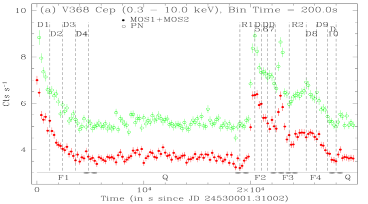
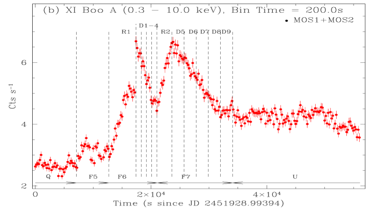
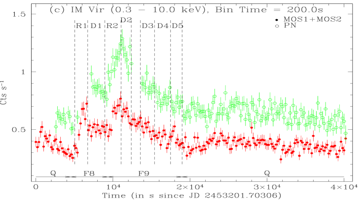
Figure 1: MOS and PN Light curves of six G-K dwarfs

Fig. 1 Continued

Figure 2: (a) MOS and PN light curves at three bands soft (0.3-0.8 keV), medium (0.8-1.6 keV), and hard(1.6-10.0 keV) and hardness ratio HR1 and HR2 curve, where HR1=medium/soft and HR2=hard/medium of V368 Cep.

Fig. 2(b) – Similar to Fig. 2 (a), but for XI Boo (only MOS)

Fig. 2(c) – Similar to Fig. 2 (a), but for IM Vir

Fig. 2(d) – Similar to Fig. 2 (a), but for V471 Tau

Fig. 2(e) – Similar to Fig. 2 (a), but for CC Eri

Fig. 2(f) – Similar to Fig. 2 (a), but for EP Eri

Figure 3: Colour-colour diagram (HR1 versus HR2) for the various time segments (Q: quiescent state, Ri(i=1,2..): rise phase, Di(i=1,2..): decay phase) observed for each source. The curves overplotted on the data are for model simulation where two temperature plasma is assumed to predict the colors (see §4.2 for details).

Fig. 3 Continued

Figure 4: Quiescent state spectra of PN data with APEC 2T model in upper subpanels of each graph. $\chi^{2}$ contributions are given in the lower subpanel of the each graph.

Figure 12: Plot of peak flare luminosity (L_Xf) versus stellar quiescent luminosity (L_Xq)

References

- [] Aschwanden M. J., Alexander, D., 2001, Sol. Phys, 204, 91
- [] Albacete Colombo J. F., Caramazza, M., Flaccomio, E., Micela, G., Sciortino, S., 2007,A&A, 474, 495
- [] Anders E., Grevesse N., 1989, Geochim. Cosmochim. Acta, 53, 197
- [] Arnaud K. A., 1996, ASPC, 101, 17
- [] Ayres T. R., Marstad N. C., Linsky J. L., 1981, ApJ, 247, 545
- [] Baliunas S. L. et al., 1995, ApJ, 438, 269
- [] Briggs K. R., Pye J. P., 2003, MNRAS, 345, 714
- [] Cayrel de Strobel G., Cayrel R., 1989, A&A, 218, 9
- [] Chugainov P.F., Lovkaya M.N., Petrov P.P., 1991, IBVS 3623
- [] Chugainov P.F., Petrov P.P., Lovkaya M.N., 1993, Izv. Krymsk. Astrofiz. Obs. 88, 29
- [] Crespo-Chacon I., Micela G., Reale F., Caramazza M., Lopez-Santiago J., Pilleteri, I., 2007,A&A, 471, 929
- [] Cutispoto G., 1992, A&AS, 95, 397
- [] Dickey J. M., Lockman F. J., 1990, ARAA, 28, 215
- [] Dennis B. R., Schwartz R. A., 1989, SoPh, 121, 75
- [] Ehle M. et al., 2004, User’s guide to XMM-Newton Science Analysis system
- [] Favata F., Micela G., Reale F., 2000a, A&A, 354, 1021
- [] Favata F., Micela G., Reale F., Sciortino S., Schmitt J.H.M.M., 2000b, A&A, 362, 628
- [] Favata F., Reale F., Micela G., Sciortino S., Maggio A., Matsumoto, H., 2000c, A&A, 353, 987
- [] Favata F., Micela G., Reale F., 2001, A&A, 375, 485
- [] Favata F., Flaccomio E., Reale F., Micela G., Sciortino S., Shang H., Stassun K. G., Feigelson E. D., 2005, ApJS, 160, 469
- [] Fekel F. C., 1997, PASP, 109, 514
- [] Garcia-Alvarez D., 2000, IrAJ, 27, 117
- [] Garcia-Alvarez D., Jevremovic D., Doyle J. G., Butler C. J., 2002, A&A, 383, 548
- [] Giardino G., Favata F., Silva B., Micela G., Reale F., & Sciortino S., 2006, A&A, 453, 241
- [] Gray D., Baliunas S., Lockwood G., Skiff B., 1996, ApJ, 465, 945
- [] Güdel M., 2004, ARA&A, 12, 71
- [] Guinan E. F., Sion E. M., 1984, AJ, 89, 1252
- [] Haisch B. M., Linsky J. L., Bornmann P. L., Stencel R. E., Antiochos S. K., Golub L., Vaiana G. S., 1983, ApJ, 267, 280
- [] Hawley S. L. et al., 1995, ApJ, 453, 464
- [] Hartmann L., Schmidtke P. C., Davis R., Dupree A. K., Raymond J., Wing R. F., 1979, ApJ, 233, L69
- [] Henry G. W., Fekel F. C., Hall D., 1995, AJ, 110, 2926
- [] Hoffleit D., Jaschek, C., 1982, The Bright Star Catalogue ((4th ed.; New Haven : Yale Univ. Obs.)
- [] Jansen F. et al., 2001, A&A, L365, 1
- [] Johns-Krull C. M., Valenti J. A., 1996, ASPC, 109, 609
- [] Kopp R. A., Poletto G., 1984, SoPh, 93, 351
- [] Kuin N. P. M., Martens P. C. H., 1982, A&A, 108, 1
- [] Kürster M., Schmitt J. H. M. M., 1996, A&A, 311, 211
- [] Laming J. M., Drake J. J., 1999, ApJ, 516, 324
- [] Landini M., Monsignori Fossi B. C., Pallavicini R., Piro L., 1986, A&A, 157, 217
- [] Maggio A., Pallavicini R., Reale F., & Tagliaferri, G., 2000, aap, 356, 62
- [] Malkov O. Y., Oblak E., Snegireva E.A., & Torra J., 2006, A&A, 446, 785
- [] Moore, R. et al., 1980, in Solar Flares, ed. P. A. Sturrock, Colorado Ass. Univ. Press, Boulder, Co., p. 341
- [] Nelson B., Young A., 1970, PASP, 82, 699
- [] Olah K., Strassmeier K. G., 2002, AN, 323, 361O
- [] Ottmann R., Schmitt J. H. M. M., 1996, A&A, 307, 813
- [] Pallavicini R., Tagliaferri G., Stella L., 1990, A&A, 228, 403
- [] Pallavicini R., Monsignori-Fossi B. C., Landini M., Schmitt, J. H. M. M., 1988, A&A, 191, 109
- [] Pallavicini R., Serio S., Vaiana G. S., 1977, ApJ, 216, 108
- [] Pillitteri I., Micela G., Reale F., Sciortino, S., 2005, A&A, 430, 155
- [] Priest E. R., 1981, in Solar flare magnetohydrodynamics, eds. E. R. Priest, Gordon and Breach Science Publishers, New York, p.1
- [] Poletto G., Pallavicini R., Kopp R. A., 1988, A&A, 201, 93
- [] Reale F., Betta R., Peres G., Serio S., McTiernan J., 1997, A&A, 325, 782
- [] Reale F., Micela G., 1998, A&A, 334, 1028
- [] Reale F., 2002, ASPC, 277, 103
- [] Reale F., Peres G., Orlando S., 2001, ApJ, 557, 906
- [] Reale F., Güdel M., Peres G., Audard M., 2004, A&A, 416, 733
- [] Reale F., 2007, A&A, 471, 271
- [] Rosner R., Tucker W. H., Vaiana G. S., 1978, ApJ, 220, 643
- [] Saar S. H., 1990, IAUS, 138, 427
- [] Schimtt J. H. M. M., Favata F., 1999, Nature, 401, 44
- [] Schimtt J. H. M. M., 1997, A&A, 318, 215
- [] Schimtt J. H. M. M., 1994, ApJS, 90, 735
- [] Serio S., Reale F., Jakimiec J., Sylwester B., Sylwester J., 1991, A&A, 241, 197
- [] Smith R. K., Brickhouse N. S., Liedahl D. A., Raymond J. C., 2001, ApJ, 556, L91
- [] Stelzer B., Neuhäuser R., Hambaryan V., 2000, A&A, 356, 949
- [] Stelzer B., Burwitz V., Audard M., Güdel M., Ness J.-U., Grosso N., Neuhäuser R., Schmitt J. H. M. M., Predehl P., Aschenbach, B., 2002, A&A, 392, 585
- [] Strassmeier K. G., Hall D. S., Fekel F. C., Scheck M., 1993, A&AS, 100, 173
- [] Strüder L. et al., 2001, A&A, 365, L18
- [] Sylwester B., Sylwester J., Serio S., Reale F., Bentley R. D., Fludra A., 1993, A&A, 267, 586
- [] Testa P., Reale F., Garcia-Alvarez D., Huenemoerder P., 2007, ApJ, 663, 1232
- [] Turner M. J. L. et al., 2001, A&A, 365, L27
- [] van den Oord G. H. J., Mewe R., 1989, A&A, 213, 245
- [] White, N. E., Culhane, J. L., Parmar, A. N., Kellett B. J., Kahn S., van den Oord G. H. J., Kuijpers J., 1986, ApJ, 301, 262
- [] Wu S. T. et al., 1986, in Energitic Phenomenon on the Sun, eds. M. Kundu& B. Woodgate, No. 2439 in NASA Conference Publication, NASA, p. 5