Quantum strategy in moving frames

Abstract

We investigate quantum strategy in moving frames by considering Prisoner’s Dilemma and propose four thresholds of $\gamma$ for two players to determine their Nash Equilibria. Specially, an interesting phenomenon appears in relativistic situation that the quantum feature of the game would be enhanced and diminished for different players whose particle’s initial spin direction are respectively parallel and antiparallel to his/her movement direction, that is, for the former the quantum feature of the game is enhanced while for the latter the quantum feature would be diminished. Thus a classical latter could still maintain his/her strictly dominant strategy (classical strategy) even if the game itself is highly entangled.

Strategy theory (or Game theory) is a branch of applied mathematics devised to analyze certain situations in which there is an interplay between parties that may have similar, opposed, or mixed interests. It draws broad attention because of its practical application in Economics, Politics, and other fields which involve cooperation or conflict Game theory . As an applied mathematical theory, strategy theory inevitably possesses its own physical properties. It is not surprising, since a game should be played through some strategies, and these strategies must be put in practice to some physical carriers. Thus the traits of the carriers under some certain physical conditions would affect the result of a game. Based on this consideration, to explore how to gain as much as reward in a game in some particular physical situations has been a popular research aspect in recent years.

In 1999, Eisert et al. proposed a novel model of quantum game in terms of the famous nonzero sum game— Prisoners’ Dilemma, in which the physical carriers are two spin-$\frac{1}{2}$ particles, and players could adopt some unitary quantum operations as strategies. Although this model was criticized for not possessing the dominance over a classical game Enk' , we find it is actually go beyond a classical game and worth studying based on the considerations that it is important for us to distinguish the difference between the equivalence of payoffs and the equivalence of strategies, and that to understand the essences of a cooperative game and a noncooperative game is of high significance in studying a game with a physical background. More interestingly, a physical carrier possesses not only quantum traits but also relativistic ones. So we are concerning on this effect by using Eisert et al.’s model. In this model, two particles (start in a produce state $\left|CC\right\rangle$) are initially entangled by a gate $\hat{J}$ to form a pairs of physical carriers of this game, and then be distributed to two players, Alice and Bob, who independently chooses a quantum strategy

$$\hat{U}(\theta,\phi)=\left(\begin{array}[]{ccc}e^{{\rm i}\phi}\cos{\theta/2}&\sin{\theta/2}\\ -\sin{\theta/2}&e^{-{\rm i}\phi}\cos{\theta/2}\\ \end{array}\right),$$ (1)

with $0\leq\theta\leq\pi$ and $0\leq\phi\leq\pi/2$. Finally, a disentangling gate $\hat{J}^{\dagger}$ is carried out and the carrier pair is measured in the computational basis. In terms of game theory, it exists a new Nash Equilibrium (NE), that is, both of the players choose strategy $\hat{Q}=\hat{U}(0,\pi/2)$, because strategy $\hat{Q}$ has the property of being Pareto optimal, and help players escape the dilemma in classical game Game theory ; Eisert .

Let us restrict the physical carriers to be two spin-$\frac{1}{2}$ particles and denote the states of the particles as: $\left|\frac{1}{2}\right\rangle=\left|\textit{C}\right\rangle=\left(\begin{array}[]{c}1\\ 0\end{array}\right)$, and $\left|-\frac{1}{2}\right\rangle=\left|\textit{D}\right\rangle=\left(\begin{array}[]{c}0\\ 1\end{array}\right)$. Meanwhile, an arbiter is needed to determine each player’s payoff by measuring the state of the two particles with a physical measurement device, and the principle of the determination is well known to both players. The players could only gain expected payoff since quantum mechanics itself is a probabilistic theory. Alice’s and Bob’s expected payoffs are given by

$$\begin{array}[]{c}\$_{A}=\textit{r}\textit{P}_{CC}+\textit{p}\textit{P}_{DD}+\textit{t}\textit{P}_{DC}+\textit{s}\textit{P}_{CD},\\ \$_{B}=\textit{r}\textit{P}_{CC}+\textit{p}\textit{P}_{DD}+\textit{s}\textit{P}_{DC}+\textit{t}\textit{P}_{CD},\\ \end{array}$$ (2)

where $P_{ab}=\left|\left\langle ab|\psi_{f}\right\rangle\right|^{2}$ ($a,b=C,D$) is the joint probability that the arbiter’s measure device would display $a,b$. We take $\textit{t}=5,\textit{r}=3,\textit{p}=1$ and $\textit{s}=0$ in this model Eisert . In this game, we assume that the arbiter moves in the x direction, Alice’s particle moves in the z direction, and Bob’s the -z direction. Thus their movements cause boosts in the direction of x, z, and -z, respectively. Thus, Alice’s and Bob’s movement directions are respectively parallel and antiparallel to their particles’ initial spin directions. We denote the boosts with each’s rapidity as $\alpha$ for the arbiter, $\delta_{A}$ for Alice, and $\delta_{B}$ for Bob.

Of course, the arbiter’s boost $\alpha$ respect to a player could also be equivalent to the player emitting the particle to the arbiter with a rapidity $-\alpha$ (that is, with $\alpha$ in the -x direction). In this case, we could further think that the arbiter is at rest, and the two players are far away from the arbiter, so they have to take part in this game by emitting their own particles to the arbiter, and the rapidity of each particle will sort of determine how much payoff the players would attain. Thus, at what speed the particle is emitted could be controlled by the player, and we name this speed-control as a relativistic operation. From our point of view, this model should be worth studying since it is a well guidance to long-distance games, and even in the near future when interstellar travel comes true, this model would also be useful.

Now we set out our game model and its process is illustrated in Fig.1, in which the Lorentz boost is introduced in Refs.Alsing ; Ahn , and $\gamma$ is a monotonic function with the measure of entanglement, indicating how much the two particles entangle. The degree of entanglement between the two particles would decrease if their momentum have distributions, say, with width. So tracing out the momentum from the Lorentz-transformation density matrix destroys some of the entanglement Gingrich . We assume the momentum of both particles to be exact, namely no distributions, thus their degree of entanglement would remain invariant under Lorentz transformation, and so does $\gamma$. When $\gamma=0$, the game’s players are separable and the game does not display any features which go beyond the classical game.

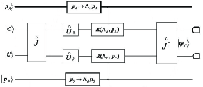
Figure 1: Process of the game model. $\hat{J}=\exp({\rm i}\gamma\hat{D}\otimes\hat{D}/2)$, $\gamma\in\left[0,\pi/2\right]$, $\hat{D}=\hat{U}(\pi,0)$, is defined in Eisert to make the two particles entangle. $R(\Lambda,\bm{p})$ is the Wigner rotation applied to a particle. $\hat{U}_{A}$ and $\hat{U}_{B}$ are operations Alice and Bob applies to her and his own particle respectively.

The Lorentz transformation $\Lambda$ results in a unitary transformation on states in the Hilbert space that $\mbox{$\left|{\Psi}\right\rangle$}\rightarrow U(\Lambda)\mbox{$\left|{\Psi}\right\rangle$}$. Thus, the state of entangled particles under the Lorentz transformation is given by

$$U(\Lambda)(\hat{U}_{A}\otimes\hat{U}_{B})\hat{J}\left|\bm{p}_{A},\!C;\bm{p}_{B},\!C\right\rangle=\sum_{a,b=C,D}k_{ab}\mbox{$\left|{\psi_{ab}}\right\rangle$},$$ (3)

$$\left|{\psi_{CC}}\right\rangle = \!\!\sqrt{\frac{(\Lambda\bm{p}_{A})^{0}}{\bm{p}_{A}^{0}}}\sqrt{\frac{(\Lambda\bm{p}_{B})^{0}}{\bm{p}_{B}^{0}}}\sum_{\sigma,\sigma^{\prime}}{D}_{\sigma,\frac{1}{2}}^{(\frac{1}{2})}\left(\emph{R}(\Lambda_{A})\right)$$ (4)

$${D}_{\sigma^{\prime},\frac{1}{2}}^{(\frac{1}{2})}\left(\emph{R}(\Lambda_{B})\right)a^{\dagger}(\bm{p}_{A_{\Lambda}},\sigma)a^{\dagger}(\bm{p}_{B_{\Lambda}},\sigma^{\prime})\mbox{$\left|{\psi_{0}}\right\rangle$},$$

$$\left|{\psi_{CD}}\right\rangle = \!\!\sqrt{\frac{(\Lambda\bm{p}_{A})^{0}}{\bm{p}_{A}^{0}}}\sqrt{\frac{(\Lambda\bm{p}_{B})^{0}}{\bm{p}_{B}^{0}}}\sum_{\sigma,\sigma^{\prime}}{D}_{\sigma,\frac{1}{2}}^{(\frac{1}{2})}\left(\emph{R}(\Lambda_{A})\right)$$ (5)

$${D}_{\sigma^{\prime},-\frac{1}{2}}^{(\frac{1}{2})}\left(\emph{R}(\Lambda_{B})\right)a^{\dagger}(\bm{p}_{A_{\Lambda}},\sigma)a^{\dagger}(\bm{p}_{B_{\Lambda}},\sigma^{\prime})\mbox{$\left|{\psi_{0}}\right\rangle$},$$

$$\left|{\psi_{DC}}\right\rangle = \!\!\sqrt{\frac{(\Lambda\bm{p}_{A})^{0}}{\bm{p}_{A}^{0}}}\sqrt{\frac{(\Lambda\bm{p}_{B})^{0}}{\bm{p}_{B}^{0}}}\sum_{\sigma,\sigma^{\prime}}{D}_{\sigma,-\frac{1}{2}}^{(\frac{1}{2})}\left(\emph{R}(\Lambda_{A})\right)$$ (6)

$${D}_{\sigma^{\prime},\frac{1}{2}}^{(\frac{1}{2})}\left(\emph{R}(\Lambda_{B})\right)a^{\dagger}(\bm{p}_{A_{\Lambda}},\sigma)a^{\dagger}(\bm{p}_{B_{\Lambda}},\sigma^{\prime})\mbox{$\left|{\psi_{0}}\right\rangle$},$$

$$\left|{\psi_{DD}}\right\rangle = \!\!\sqrt{\frac{(\Lambda\bm{p}_{A})^{0}}{\bm{p}_{A}^{0}}}\sqrt{\frac{(\Lambda\bm{p}_{B})^{0}}{\bm{p}_{B}^{0}}}\sum_{\sigma,\sigma^{\prime}}{D}_{\sigma,-\frac{1}{2}}^{(\frac{1}{2})}\left(\emph{R}(\Lambda_{A})\right)$$ (7)

$${D}_{\sigma^{\prime},-\frac{1}{2}}^{(\frac{1}{2})}\left(\emph{R}(\Lambda_{B})\right)a^{\dagger}(\bm{p}_{A_{\Lambda}},\sigma)a^{\dagger}(\bm{p}_{B_{\Lambda}},\sigma^{\prime})\mbox{$\left|{\psi_{0}}\right\rangle$}.$$

where $\left|{\psi_{0}}\right\rangle$ is the Lorentz invariant vacuum state, and

$$k_{CC} = e^{{\rm i}(\phi_{A}+\phi_{B})}c_{\theta_{A}}c_{\theta_{B}}c_{\gamma}+{\rm i}s_{\theta_{A}}s_{\theta_{B}}s_{\gamma},$$ (8)

$$k_{CD} = -e^{{\rm i}\phi_{A}}c_{\theta_{A}}s_{\theta_{B}}c_{\gamma}+{\rm i}e^{-{\rm i}\phi_{B}}s_{\theta_{A}}c_{\theta_{B}}s_{\gamma},$$ (9)

$$k_{DC} = -e^{{\rm i}\phi_{B}}s_{\theta_{A}}c_{\theta_{B}}c_{\gamma}+{\rm i}e^{-{\rm i}\phi_{A}}c_{\theta_{A}}s_{\theta_{B}}s_{\gamma},$$ (10)

$$k_{DD} = s_{\theta_{A}}s_{\theta_{B}}c_{\gamma}+{\rm i}e^{-{\rm i}(\phi_{A}+\phi_{B})}c_{\theta_{A}}c_{\theta_{B}}s_{\gamma}.$$ (11)

For simplicity, we denote

$$c_{x}=\cos\frac{x}{2},\quad s_{x}=\sin\frac{x}{2},$$ (12)

where $x$ can be taken as $\theta_{A}$, $\theta_{B}$ and $\gamma$ as well as so-called Wigner angle $\Omega_{A}$ and $\Omega_{B}$ respectively with Alice’s and Bob’s particles. Note that a particle’s Wigner angle is determined by the rapidities of itself ($\delta$) and the arbiter ($\alpha$) Alsing Ahn ,

$$\Omega_{\tau}=\arctan\frac{\sinh\alpha\sinh\delta_{\tau}}{\cosh\alpha+\cosh\delta_{\tau}},\tau=A,B.$$ (13)

The final state measured by the arbiter is $\left|\psi_{f}\right\rangle=\hat{J}^{\dagger}U(\Lambda)(\hat{U}_{A}\otimes\hat{U}_{B})\hat{J}\left|\bm{p}_{A},C;\bm{p}_{B},C\right\rangle$. We have

$$\left(\begin{array}[]{c}\mathfrak{p}_{1}\\ \mathfrak{p}_{2}\\ \mathfrak{p}_{3}\\ \mathfrak{p}_{4}\end{array}\right)=\left(\begin{array}[]{cccc}\omega_{1}&\omega^{*}_{2}&-\omega^{*}_{3}&-\omega_{4}\\ -\omega^{*}_{2}&\omega_{1}&\omega_{4}&-\omega_{3}\\ \omega^{*}_{3}&\omega_{4}&\omega_{1}&-\omega_{2}\\ -\omega_{4}&\omega^{*}_{3}&-\omega^{*}_{2}&\omega_{1}\end{array}\right)\left(\begin{array}[]{c}k_{CC}\\ k_{CD}\\ k_{DC}\\ k_{DD}\end{array}\right),$$ (14)

where $\omega_{1}=c_{\gamma}c_{\Omega_{A}}c_{\Omega_{B}}+{\rm i}s_{\gamma}s_{\Omega_{A}}s_{\Omega_{B}}$, $\omega_{2}=c_{\gamma}c_{\Omega_{A}}s_{\Omega_{B}}+{\rm i}s_{\gamma}s_{\Omega_{A}}c_{\Omega_{B}}$, $\omega_{3}=c_{\gamma}s_{\Omega_{A}}c_{\Omega_{B}}+{\rm i}s_{\gamma}c_{\Omega_{A}}s_{\Omega_{B}}$, and $\omega_{4}=c_{\gamma}s_{\Omega_{A}}s_{\Omega_{B}}+{\rm i}s_{\gamma}c_{\Omega_{A}}c_{\Omega_{B}}$, and $*$ denotes complex conjugation. Thus we get ${P}_{CC}=\left|\mathfrak{p}_{1}\right|^{2}$, ${P}_{CD}=\left|\mathfrak{p}_{2}\right|^{2}$, ${P}_{DC}=\left|\mathfrak{p}_{3}\right|^{2}$, and ${P}_{DD}=\left|\mathfrak{p}_{4}\right|^{2}$.

Actually, how much the two particles are initially entangled would be essential to this game model, since $\gamma$ induces some features which go beyond the classical game. Du et al. found two thresholds of $\gamma$ in the Quantum Prisoners’ Dilemma— $\gamma_{th1}=\arcsin{\sqrt{1/5}}$ and $\gamma_{th2}=\arcsin{\sqrt{2/5}}$, which separate the game into three regions: classical region ($\gamma\in\left[0,\gamma_{th1}\right)$), intermediate region ($\gamma\in\left[\gamma_{th1},\gamma_{th2}\right)$), and fully quantum region ($\gamma\in\left[\gamma_{th2},\pi/2\right]$), see Ref.Du Du' . According to Du, the classical region means in this domain, the game behaves classically, i.e., the NE of the game is $\hat{D}\otimes\hat{D}$; in the quantum region, the game is similar to the maximally entangled one in Eisert’s Letter Eisert that $\hat{Q}\otimes\hat{Q}$ becomes the new NE and has the property to be Pareto Optimal; while the intermediate region possesses compatibility to $\hat{D}$ and $\hat{Q}$, where $\hat{D}\otimes\hat{D}$ is no longer the NE because each player could improve his/her payoff by unilaterally deviating from the strategy $\hat{D}$, thus two Nash Equilibria (NE’s) $\hat{D}\otimes\hat{Q}$ and $\hat{Q}\otimes\hat{D}$ emerge Du .

In order to explore the relativistic-quantum features of this game, we take four situations as examples, in which $4$-kinds of payoffs are considered for each player— (a) Alice moves at low speed (AL) & Bob moves at low speed (BL), (b) Alice moves at low speed (AL) & Bob moves at high speed (BH), (c) Alice moves at high speed (AH) & Bob moves at low speed (BL), and (d) Alice moves at high speed (AH) & Bob moves at high speed (BH); and $G_{1}:=\$(\hat{D}\otimes\hat{D})$, $G_{2}:=\$(\hat{Q}\otimes\hat{D})$, $G_{3}:=\$(\hat{D}\otimes\hat{Q})$, and $G_{4}:=\$(\hat{Q}\otimes\hat{Q})$. And we concentrate our discussion to a simple but typical strategy set $S=\{\hat{D},\hat{Q}\}$, since $\hat{D}=\hat{U}(\pi,0)$ is a classical spin-rotating operation which could be implemented by sort of classical equipments, while $\hat{Q}=\hat{U}(0,\pi/2)$ is a purely phase-controlling operation which could only be implemented by a quantum gate. It is an essential difference between these two strategies. Thus, there are at most six thresholds of $\gamma$ ($\gamma_{\mu\nu},\mu,\nu=1,2,3,4$, with $\mu<\nu$, where $\gamma_{\mu\nu}$ is the point where $G_{\mu}=G_{\nu}$) for each player’s payoff in each situation. Among these $\gamma_{\mu\nu}$, there are two thresholds are essential for each player— for Alice, they are $\gamma_{12}$ and $\gamma_{34}$, we denote them as $\gamma^{A}_{12}$ and $\gamma^{A}_{34}$; similarly, for Bob, they are $\gamma^{B}_{13}$ and $\gamma^{B}_{24}$. These four thresholds are essential because they demonstrate Alice’s and Bob’s strictly dominant strategies (SDS) for different $\gamma\in\left[0,\frac{\pi}{2}\right]$ Game theory . Fig.2 illustrates Alice’s and Bob’s payoffs in the four situations. Here, as for low and high speed we can respectively take $\Omega_{\tau}=\frac{\pi}{16}$ and $\Omega_{\tau}=\frac{7\pi}{16}$. As is mentioned in Ref.Ahn , $\Omega_{\tau}$ is a monotonic function with player $\tau$’s and the arbiter’s speeds. Thus in this example, $\Omega_{\tau}=\frac{\pi}{16}$ corresponds to arbiter’s speed 0.01c and $\tau$’s speed 0.001c, while $\Omega_{\tau}=\frac{7\pi}{16}$ corresponds to arbiter’s speed 0.97c and $\tau$’s speed 0.908c, where c is the light-speed. The arbiter’s speed is equivalent to the same speed that the player emits his/her particle in the -x direction, as mentioned above.

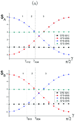
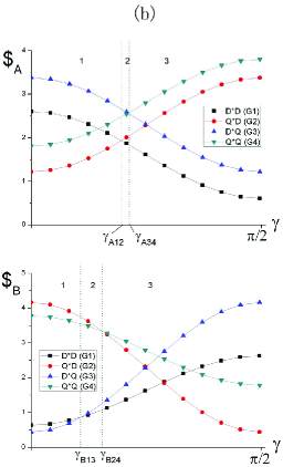
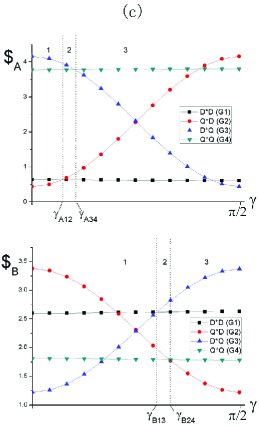
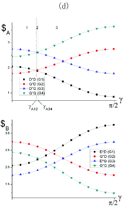
Figure 2: (Color online) Alice’s and Bob’s payoffs in 4 situations— (a) AL & BL, (b) AL & BH, (c) AH & BL, and (d) AH & BH.

In Fig.2, we name the region where $\gamma^{A}_{12}<\gamma<\gamma^{A}_{34}$ Alice’s transition region ($\mathcal{T}_{A}$), and where $\gamma^{B}_{13}<\gamma<\gamma^{B}_{24}$ Bob’s transition region ($\mathcal{T}_{B}$). If $\gamma$ is on the left side of $\mathcal{T}_{\tau}$, then $\tau$’s SDS is $\hat{D}$ (purely classical strategy); if $\gamma$ is on the right side of $\mathcal{T}_{\tau}$, the SDS is $\hat{Q}$ (purely quantum strategy); while if $\gamma$ is in $\mathcal{T}_{\tau}$, $\tau$ would have no SDS, but the NE still exist. Game theory proves that the combination of each player’s SDS must be the NE of the game, but a NE may not be the combination of each’s SDS Game theory . From Fig.2, we could see that in some situations, $\mathcal{T}_{A}$ and $\mathcal{T}_{B}$ overlap partially with each other, and in the overlapping region, two new NE’s $\hat{D}\otimes\hat{Q}$ and $\hat{Q}\otimes\hat{D}$ appear, although there is no SDS exists for each player. On the other hand, if $\gamma$ is in $\mathcal{T}_{A}$ but not in $\mathcal{T}_{B}$, Bob has SDS $\hat{D}$ or $\hat{Q}$, but Alice has not, in this case, the NE is $\hat{Q}\otimes\hat{D}$ or $\hat{D}\otimes\hat{Q}$, that is to say, Alice should choose the strategy opposite to Bob’s SDS. It is similar to the case that $\gamma$ is in $\mathcal{T}_{B}$ but not in $\mathcal{T}_{A}$. What is noteworthy is the highly relativistic situation in Fig.2.(d): $\Omega_{A}=\Omega_{B}=\frac{7\pi}{16}$. In this case, there is no transition region for Bob, and for all $\gamma\in\left[0,\frac{\pi}{2}\right]$, Bob’s SDS is $\hat{D}$, that is to say, when Alice’s and Bob’s particles both move at very high speed, the game behaves classically for Bob, even if he is highly entangled with Alice. It is an interesting phenomenon that the relativistic operations would diminish the quantum feature of the game. Fig.3 shows the area where Bob’s SDS is $\hat{D}$ for all $\gamma\in\left[0,\frac{\pi}{2}\right]$, i.e., where the relativistic operation entirely eliminate the quantum feature of the game for Bob.

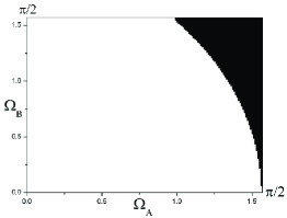
Figure 3: The shadowed area indicates the situation in which Bob’s SDS is always $\hat{D}$ in spite of how much the two particles are entangled.

In fact, the four thresholds vary with $\Omega_{A}$ and $\Omega_{B}$ as

$$\gamma^{A}_{12}\!=\!\arcsin\!{\sqrt{\frac{c^{2}_{\Omega_{A}}c^{2}_{\Omega_{B}}\!-\!2s^{2}_{\Omega_{A}}s^{2}_{\Omega_{B}}\!+\!2c^{2}_{\Omega_{A}}s^{2}_{\Omega_{B}}\!-\!s^{2}_{\Omega_{A}}c^{2}_{\Omega_{B}}}{5c^{2}_{\Omega_{A}}c^{2}_{\Omega_{B}}\!-\!5s^{2}_{\Omega_{A}}s^{2}_{\Omega_{B}}\!+\!3c^{2}_{\Omega_{A}}s^{2}_{\Omega_{B}}\!+\!2s^{2}_{\Omega_{A}}c^{2}_{\Omega_{B}}}}},$$ (15)

$$\gamma^{A}_{34}\!=\!\arcsin\!{\sqrt{\frac{2c^{2}_{\Omega_{A}}c^{2}_{\Omega_{B}}\!-\!s^{2}_{\Omega_{A}}s^{2}_{\Omega_{B}}\!+\!c^{2}_{\Omega_{A}}s^{2}_{\Omega_{B}}\!-\!2s^{2}_{\Omega_{A}}c^{2}_{\Omega_{B}}}{5c^{2}_{\Omega_{A}}c^{2}_{\Omega_{B}}\!-\!5s^{2}_{\Omega_{A}}s^{2}_{\Omega_{B}}\!+\!3c^{2}_{\Omega_{A}}s^{2}_{\Omega_{B}}\!+\!2s^{2}_{\Omega_{A}}c^{2}_{\Omega_{B}}}}},$$ (16)

$$\gamma^{B}_{13}\!=\!\arcsin\!{\sqrt{\frac{c^{2}_{\Omega_{A}}c^{2}_{\Omega_{B}}\!-\!2s^{2}_{\Omega_{A}}s^{2}_{\Omega_{B}}\!-\!c^{2}_{\Omega_{A}}s^{2}_{\Omega_{B}}\!+\!2s^{2}_{\Omega_{A}}c^{2}_{\Omega_{B}}}{5c^{2}_{\Omega_{A}}c^{2}_{\Omega_{B}}\!-\!5s^{2}_{\Omega_{A}}s^{2}_{\Omega_{B}}\!-\!3c^{2}_{\Omega_{A}}s^{2}_{\Omega_{B}}\!-\!2s^{2}_{\Omega_{A}}c^{2}_{\Omega_{B}}}}},$$ (17)

$$\gamma^{B}_{24}\!=\!\arcsin\!{\sqrt{\frac{2c^{2}_{\Omega_{A}}c^{2}_{\Omega_{B}}\!-\!s^{2}_{\Omega_{A}}s^{2}_{\Omega_{B}}\!-\!2c^{2}_{\Omega_{A}}s^{2}_{\Omega_{B}}\!+\!s^{2}_{\Omega_{A}}c^{2}_{\Omega_{B}}}{5c^{2}_{\Omega_{A}}c^{2}_{\Omega_{B}}\!-\!5s^{2}_{\Omega_{A}}s^{2}_{\Omega_{B}}\!-\!3c^{2}_{\Omega_{A}}s^{2}_{\Omega_{B}}\!-\!2s^{2}_{\Omega_{A}}c^{2}_{\Omega_{B}}}}}.$$ (18)

always with $\gamma^{A}_{12}<\gamma^{A}_{34}$ and $\gamma^{B}_{13}<\gamma^{B}_{24}$. We plot these four thresholds in Fig.4. In particular, when Alice, Bob and the arbiter are all at rest, i.e., $\Omega_{A}=\Omega_{B}=0$, $\mathcal{T}_{A}$ and $\mathcal{T}_{B}$ overlap entirely with each other. In this case, $\gamma^{A}_{12}=\gamma^{B}_{13}=\gamma_{th1}$ in Du’s paper Du , and $\gamma^{A}_{34}=\gamma^{B}_{24}=\gamma_{th2}$, thus two NE’s emerge in the overlapping region.

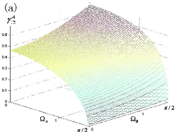
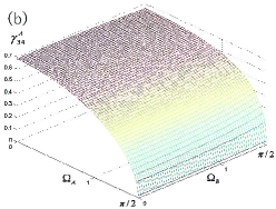
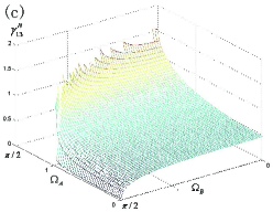
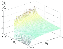
Figure 4: The four thresholds $\gamma^{A}_{12}$, $\gamma^{A}_{34}$, $\gamma^{B}_{13}$ and $\gamma^{B}_{24}$, which divide the game into three regions respectively according to $\gamma$, and determine the Nash Equilibrim of this game.

Finally, we could see in Fig.4.(b) that for Alice, $\gamma^{A}_{34}<\frac{\pi}{2}$ in all situations, and $\gamma^{A}_{34}\rightarrow 0$ when $\Omega_{A}\rightarrow\frac{\pi}{2}$, i.e., when Alice’s particle moves at very high speed, her SDS would be $\hat{Q}$ even if the two particles are entirely separable; while in Fig.4.(c), $\gamma^{B}_{13}>\frac{\pi}{2}$ in some situations, where the quantum feature of the game is entirely eliminated for Bob, so his SDS is $\hat{D}$ even if the two particles are entirely entangled. That is to say, in the same game, the relativistic operations enhance the quantum feature of the game for Alice, but diminish it for Bob.

In summary, we have demonstrated that some new and interesting features appear if classical games such as Prisoners’ Dilemma are extended to the quantum and relativistic domain, in which the initial symmetry of this game is broken by the respect movements of the two players. We also propose four thresholds for Alice and Bob, which divide the game into three regions in which different strictly dominant strategies emerge, and how Nash Equilibrium is determined in different situations. Moreover, a interesting phenomenon appears in relativistic situation that the relativistic operations could enhance the quantum feature of the game for the player whose particle’s initial spin direction is parallel to its movement direction (Alice), but diminish it for the one whose particle’s initial spin direction is antiparallel to its movement direction (Bob), i.e., the respect movements of Alice, Bob and the arbiter determine “how quantum” the game is for each player. We believe these properties would be useful to guide remote games in the future and that extending game theory to quantum and relativistic domain would lead us to understand the physical essence of game theory.

We are grateful to all the collaborators of our quantum theory group in the institute for theoretical physics of our university. We thank Prof. Lewenstein and Zeyang Liao for triggering and useful discussion. This work was supported by the National Natural Science Foundation of China under Grant No. 60573008.

References

• (1) For an introduction, see, e.g., R.B. Myerson, GAme Theory: An Analysis of Conflict (MIT Press, Cambridge, MA, 1991), D. Fudenberg, J. Tirole, Game theory (The MIT Press, Cambridge, Massachusetts, 1991).
• (2) D.A. Meyer, Phys. Rev. Lett. 82, 1052 (1999).
• (3) L.Goldenberg, L.Vaidman, S.Wiesner, Phys. Rev. Lett. 82, 3356 (1999).
• (4) J. Eisert, M. Wilkens, and M. Lewenstein, Phys. Rev. Lett. 83, 3077 (1999).
• (5) S.J. van Enk and R. Pike, Phys. Rev. A. 66, 024306 (2002).
• (6) R.M. Gingrich and C. Adami, Phys. Rev. Lett. 89, 270402 (2002).
• (7) E. Wigner, Ann. Math. 149, 40 (1939).
• (8) P.M. Alsing and G.J. Milburn, Quantum Inf. Comput. 2, 487 (2002).
• (9) D.Ahn, H.J. Lee, Y.H. Moon, S.W. Hwang, Phys. Rev. A. 67, 012103 (2003).
• (10) A. Peres, P.F. Scudo, D.R. Terno, Phys. Rev. Lett. 88, 230402 (2002).
• (11) L.H. Ryder, Quantum field theory (Cambridge University Press, New York, 1996).
• (12) M. Czachor, Phys. Rev. A. 55, 72 (1997).
• (13) S. Weinberg, The Quantum Theory of Fields I (Cambrige University Press, New York, 1995).
• (14) H. You, A.M. Wang, X. Yang, et al., Phys. Lett. A. 333 (2004) 389-394.
• (15) F.R. Halpern, Special Relativity and Quantum Mechanics (Prentice-Hall, Englewood Cliffs, NJ, 1968).
• (16) A. Peres, D.R. Terno, Rev. Mod. Phys. 76 (2004) 93.
• (17) J. Du et al., Phys. Lett. A. 289 (2001) 9-15.
• (18) J. Du et al., Phys. Rev. Lett. 88, 137902 (2002).
• (19) S. Hill and W.K. Wootters, Phys. Rev. Lett. 78, 5022 (1997).
• (20) S.J. van Enk, Phys. Rev. Lett. 84, 789 (2000).
• (21) A. Iqbal and A.H. Toor, Phys. Rev. A. 65, 022306 (2002)
• (22) S.C. Benjamin and P.M. Hayden, Phys. Rev. Lett. 87, 069801 (2001)
• (23) J.Eisert, M.Wilkens, M.Lewenstein, Phys. Rev. Lett. 87, 069802 (2001)