Regular motions in double bars. II. Survey of trajectories and 23 models

Abstract

We show that stable double-frequency orbits form the backbone of double bars, because they trap around themselves regular orbits, as stable closed periodic orbits do in single bars, and in both cases the trapped orbits occupy similar volume of phase-space. We perform a global search for such stable double-frequency orbits in a model of double bars by constructing maps of trajectories with initial conditions well sampled over the available phase-space. We use the width of a ring sufficient to enclose a given map as the indicator of how tightly the trajectory is trapped around a double-frequency orbit. We construct histograms of these ring widths in order to determine the fraction of phase-space occupied by ordered motions. We build 22 further models of double bars, and we construct histograms showing the fraction of the phase-space occupied by regular orbits in each model. Our models indicate that resonant coupling between the bars may not be the dominant factor reducing chaos in the system.

1 Introduction

In this series of papers, we study the dynamics of galaxies with double bars, i.e. systems, where a small bar is nested inside a large-scale outer bar, and the two bars rotate with two different pattern speeds. Such double bars belong to a general class of oscillating potentials, with the oscillation period being the time between two consecutive alignments of the bars. An oscillating system in $N$ dimensions is equivalent to an autonomous system in $N+1$ dimensions (e.g. Lichtenbeg & Lieberman 1992, Louis & Gerhard 1988). In the first paper of the series (Maciejewski & Athanassoula 2007, hereafter Paper I) we showed that double bars have no continuous families of closed periodic (single-frequency) orbits; instead, their fundamental kind of orbits have two frequencies. These double-frequency orbits constitute a subset of the regular orbits in the plane of a doubly barred galaxy and, if stable, they are surrounded by regular (three-frequency) orbits in the same way as stable closed periodic orbits in a single bar are surrounded by two-frequency orbits. In both cases, the trapped regular orbits oscillate around the parent orbit. In Paper I, we showed an example of the parent stable double-frequency orbit in double bars (fig.2 in Paper I), and an example of a regular orbit that is trapped around it (the right panels of fig.1 in Paper I).

Trajectories in a pulsating potential are difficult to study, because they do not close in any reference frame. Some information about their eccentricity and their alignment with the bars can be obtained from measuring their maximum extent in the direction of bar’s major and minor axes in the frame of the bar (El-Zant & Shlosman 2003). Maciejewski & Sparke (2000, hereafter MS00) proposed another way to study such trajectories. They used maps, each built out of a discrete set of points on a given trajectory separated by the interval equal to the oscillation period. In double bars, maps of trajectories are generated by writing the position on the particle’s trajectory every time interval equal to the relative period of the bars. In Paper I, we showed that maps of double-frequency orbits created by this construction form closed curves, which we call loops, following Maciejewski & Sparke (1997), who originally defined and named these curves. Loops in double bars can be studied in the same way as closed periodic orbits in the frame of a single bar. Regular orbits trapped around double-frequency orbits (referred to in this paper as trapped trajectories) map onto rings enclosing the loops. One can follow the transformation of a loop or a ring as bars rotate through one another to see whether it supports either bar, and we follow this approach here to study trajectories in the pulsating potential of double bars. Some trajectories in double bars can be trapped by one bar for a limited period of time, and then move to chaotic region of phase space before being trapped by another bar. In our approach, such trajectories will not show as trapped by any bar, and therefore we may underestimate the orbital support of double bars.

As in Paper I, we limit ourselves to studying trajectories in the plane of the galaxy, since we extensively use the concept of the ring in the maps of trajectories, which is well defined only in the plane of the galaxy. Consequently, we consider only trajectories with no initial velocity component in the direction perpendicular to the galactic plane. Stable double-frequency orbits in double bars can be found by searching for trajectories whose maps can be enclosed by rings of the smallest possible width. As we showed in Paper I, the smaller the ring width in the map of a trajectory, the less oscillations in this trajectory around the parent orbit. Here, we explore a multi-dimensional phase-space of initial conditions, in which families of double-frequency orbits can be localized by one-dimensional stretches of near-zero ring widths. We start the search for families of double-frequency orbits in double bars from Model 2 of MS00, which we will call the Reference Model in this paper. We chose this starting point because the Reference Model is so far the best understood dynamically plausible model of double bars, i.e. the loops there follow the motion of the outer and the inner bar throughout the whole extent of the bars. In this model, we explore thoroughly the phase-space of initial conditions, achieving completeness similar to that of surfaces of section in a single bar, in order to find all orbital families that may play a role in supporting double bars. We also construct other models of double bars, for which we explore the extent of only major families of double-frequency orbits. In each model, we estimate the fraction of the phase-space occupied by regular motions. In double bars, a piling up of resonances created by each bar is likely to occur, which leads to considerable chaotic zones. In order to sustain the two bars dynamically, a resonant coupling may occur, as that proposed by Tagger et al. (1987) and Sygnet et al. (1988), so that a resonance generated by one bar overlaps with another caused by the other bar. Here we estimate the extent of chaos both in resonantly coupled and uncoupled double bars.

In Section 2, we compare the distribution of ring-widths in maps of trajectories in a single bar and in double bars using the Reference Model. In order to determine the fraction of the phase-space occupied by ordered motions, we construct histograms of the ring width. In Section 3, we analyze maps at various relative positions of the bars, and we search for asymmetric loops by considering initial velocities with a radial component. In Section 4, we build models whose characteristics depart from those of the Reference Model, and study regular motions in these models. By comparing ring-width diagrams and histograms we select models of double bars that are most plausible dynamically. In Section 5, we discuss the orbital response to varying parameters of the models, and we compare the predictions of our models with N-body simulations.

2 Comparison of regular motions in single and double bars

In a single bar, there are four initial conditions for a trajectory in the galaxy plane: two for the initial position and two for the initial velocity. Since one integral of motion, the Jacobi integral, is conserved in a rotating bar, three initial conditions are needed for a trajectory with a given Jacobi integral. If this trajectory covers the whole 2$\pi$ angle in azimuth, no generality is lost if its origin is assumed to be at one given azimuthal angle, e.g. on the minor axis of the bar. This reduces the number of initial conditions to two, and allows the study of motions in a single bar by constructing surfaces of section.

In a double bar, there is one more initial condition for a trajectory in the galactic plane, the initial relative angle of the bars, which brings the total number of initial conditions to five. Moreover, the Jacobi integral is no longer conserved, hence surfaces of section cannot be constructed. Like in a single bar, the number of initial conditions can be reduced by one after assuming the initial azimuthal angle of the trajectory. As a first step, we start the trajectory on the minor axis of the aligned bars, hence we fix one more initial condition: the relative angle of the bars. Later on, we will release this assumption. We start with the bars aligned, because only for bars aligned (parallel) or perpendicular, the potential preserves the symmetry with respect to the bars’ axes, present in the case of a single bar. Nevertheless, this still leaves us with three independent initial conditions, instead of two in a single bar, and we have to explore the phase-space of initial conditions differently.

We start our search of fundamental orbits in double bars with exploration of trajectories that have no initial radial velocity component, because in a single bar the fundamental x1 and x2 orbital families (we use the generally accepted notation from Contopoulos & Papayannopoulos 1980), and many other important families there are symmetric with respect to the axes of the bar and have no radial velocity component when crossing the minor axis. With this constraint, we expect to recover double-frequency orbits, whose maps are symmetric around the axes of the bars when the two bars are parallel. An additional benefit of imposing this constraint is that we are left with only two free parameters to vary for the initial conditions: the starting location of the particle on the minor axis of the aligned bars, and the value of its initial tangential velocity.

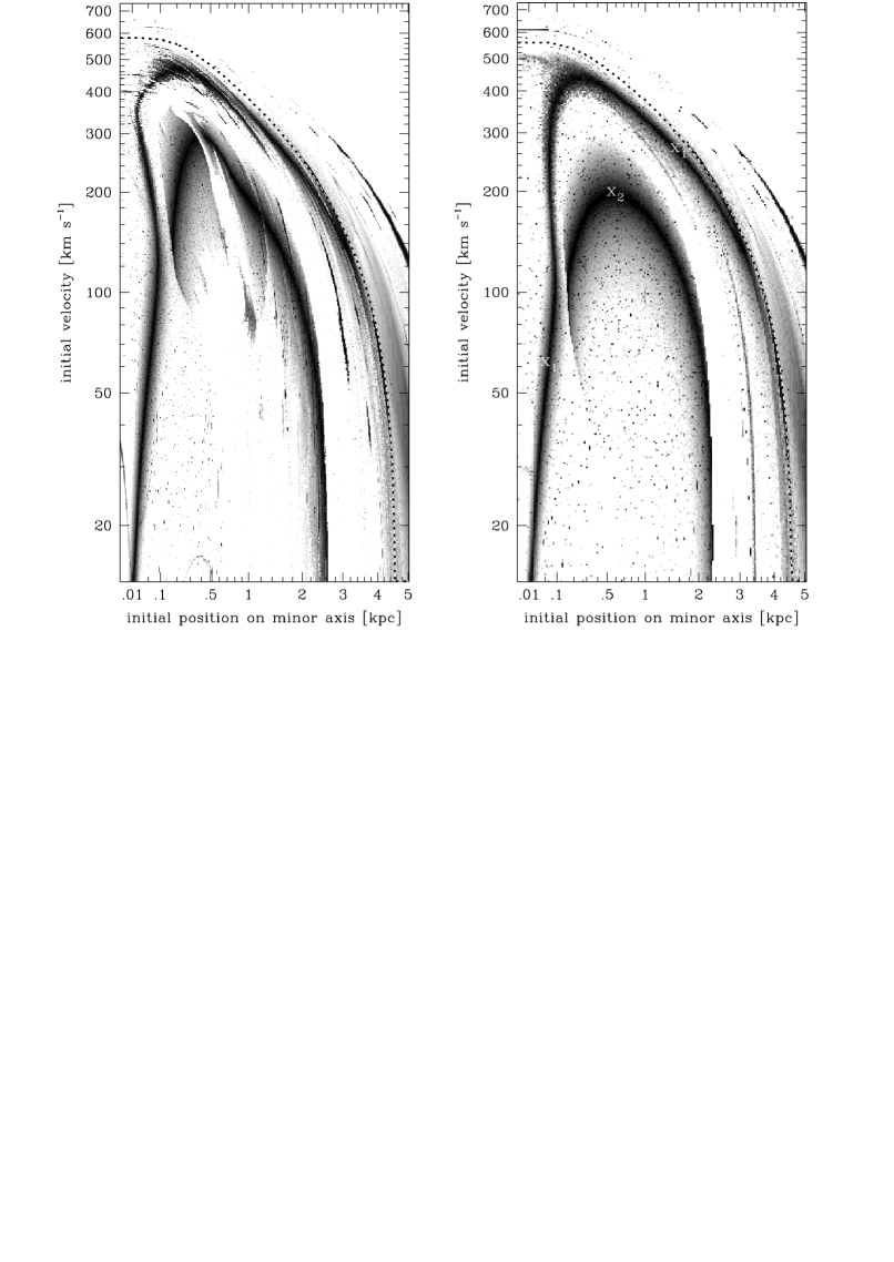
Figure 1: Left-hand panel: Width of the ring enclosing maps of trajectories in the Reference Model, plotted in greyscale as a function of the particle’s initial position on the minor axis of the aligned bars, and of the value of its initial velocity, perpendicular to this axis. Darker color means smaller width, and widths above 50 per cent of the ring’s average radius are shown in white. The white line with black dots marks values of initial conditions above which energetics allows the particle to pass the L1 Lagrange point of the outer bar (see text). Right-hand panel: Same as in the left-hand panel, but for the trajectories in a single bar generated from the Reference Model by incorporating the mass of the inner bar into the spheroid. Two dark stripes corresponding to the trajectories trapped around the x1 and x2 periodic orbits are marked.

2.1 The double-bar Reference Model and the single-bar model derived from it

Our Reference Model (Model 2 in MS00), consists of a spheroid, a disc and two bars, with, respectively, a Hubble, a Kuzmin-Toomre and a Ferrers profile, as in the single bar models of Athanassoula (1992a). The exponent in the Ferrers formula is 2. The L1 Lagrangian point for the outer, main bar is located 6 kpc from the galaxy centre. It roughly corresponds to the corotation radius of the outer bar. The semi-major axis of the main bar is also 6 kpc, hence the bar is rapidly rotating. The semi-major axis of the inner, secondary bar is 1.2 kpc, hence its linear size is 5 times smaller than that of the outer bar. The axial ratios are 2.5 for the outer bar and 2 for the inner bar. The quadrupole moment of the outer bar is $4.5\times 10^{10}$ M_⊙kpc², with the maximum ratio of the tangential to the radial force from the total mass distribution being about 20 per cent, which indicates a medium-strength bar. The mass of the inner bar is 15 per cent of that of the outer one. Pattern speeds of the bars are not commensurate (36.0 km s^-1 kpc^-1 for the big bar, and 110.0 km s^-1 kpc^-1 for the small one). This last value places the corotation of the inner bar at 2.2 kpc, at the location of the Inner Lindblad Resonance of the outer bar, hence a resonant coupling exists between the bars in this model. On the other hand, the corotation of the inner bar is far beyond its end, hence the inner bar is not rotating rapidly.

Mass distribution in our models is constructed by assuming the parameters of the disk and the spheroid, and then extracting from the spheroid the mass that is needed to create bars of the required size, quadrupole moment and density profile. In this way, the total mass of the system remains constant, and all models have the same total mass. For the single-bar model derived from the Reference Model, the mass of the secondary bar is not extracted, and it remains in the spheroid.

2.2 The ring-width diagrams

As already mentioned at the start of Section 2, we first reduce the number of initial conditions of trajectories that we want to explore to two: the initial position along the minor axis of the aligned bars, and the initial velocity perpendicular to this axis. Now, we can construct two-dimensional diagrams of any variable that characterizes the resulting trajectory, as a function of the values of initial conditions plotted on the two axes of the diagram. The variable that allows finding double-frequency orbits and trajectories trapped around them in double bars is the width of the ring that encloses the map of the trajectory. The minimal width indicates a double-frequency orbit, and small widths for adjacent initial conditions indicate trajectories trapped around the double-frequency orbit.

We construct the maps from trajectories followed for 399 alignments of the bars, therefore each map consists of 400 points. For each map we measure the width of the ring within which these points fall. The method of calculating the ring width, based on the method proposed by MS00, is explained in detail in Paper I. To summarize it, the ring width is defined as the median radial spread of points among a number (usually 40) of equal azimuthal sectors covering the whole 2$\pi$ angle, normalized by the average radial coordinate of the points that constitute the map. When this normalized ring width is much smaller than 1, one may expect a trapped trajectory, while there is no sign of the trajectory being trapped when it is close to 1. Moreover, in Paper I, we showed that the numerical value of the width of the ring indicates how tightly the particle is trapped around its parent double-frequency orbit.

In the left panel of Fig.1, we show the diagram of the ring width for the Reference Model. We sample the space of initial conditions for 400 starting positions and 800 starting velocity values, hence 320,000 ring widths are displayed in greyscale. The ring width is measured for the maps obtained at the moments when the major axes of the bars overlap. Darker shading corresponds to smaller widths, while widths higher than 0.5 are left white (trajectories that map onto rings of widths higher than 0.5 are unlikely to be trapped around regular orbits – see fig.5 in Paper I). This plot is essentially fig.8a from MS00, albeit at a much higher resolution. Dark shadings form clear stripes, darkest in their centres. Taking cuts through these stripes for a constant initial position on the minor axis will produce diagrams of ring width like the one from the lower panel of fig.5 in Paper I. In Paper I, we showed that trajectories entering that diagram are trapped around a double-frequency orbit, whose map has the smallest ring width. Therefore in the two-dimensional representation of Fig.1, the darkest lines in the interior of the stripes are likely to correspond to maps of double-frequency orbits, since the measured ring width of the loop is very small. The remainder of each stripe that surrounds those lines indicates regular trajectories trapped around those double-frequency orbits. In Paper III (Maciejewski et al. 2008, in preparation), we will prove that this is in fact the case.

The main families of loops in double bars are related to the main orbital families in a single bar (MS00). In the right panel of Fig.1, we show the diagram of the ring width for the single-bar model derived from the Reference Model, as described in Section 2.1. The mapping of trajectories is still done every time period equal to the relative period of the bars in the Reference Model. We do this for consistency with the double bar work, although in a single bar the frequency of writing is irrelevant, since the loop is identical to the closed periodic orbit. Like in the case of double bars, we followed the particle for a time equal to 399 relative periods of the bars in the Reference Model, writing its position 400 times at equal time intervals.

MS00 showed to which orbits in a single bar various features in the ring-width diagram correspond, and we will expand this analysis in Paper III. Here we only summarize that trajectories with initial conditions from the darkest ’spine’ of the stripe forming the lower arch in the single-bar diagram in Fig.1 belong to the x2 orbital family. The stripe that makes the upper arch represents trajectories trapped around the x1 orbital family and orbital families related to it. A stripe of small ring width, emerging from the right side of the box at a velocity about 120 km s^-1corresponds to orbits beyond the corotation of the bar, belonging to the outer 2:1 orbital family (see e.g. fig.11 in Sellwood & Wilkinson 1993). There are also other, secondary features in the ring-width diagram, like grey stripes that do not include ring widths near zero, but their importance for the dynamics of the system is small.

When comparing the two diagrams in Fig.1, one can notice that the two dark arcs, marking the x1 and x2 orbital families in the single bar, occur at similar locations in the diagram for the double bar, and they have similar appearance there. This confirms the finding of MS00 that in double bars there are double-frequency orbits that correspond to closed periodic orbits in single bars. Thus, one can use the diagram from the left panel of Fig.1 to single out families of double-frequency orbits. This will be done in Paper III. Major double-frequency orbits map onto loops, whose appearance was given in MS00.

Despite general similarities, there are also significant differences between the diagrams in Fig.1. The diagram for the double bar looks less regular, with a number of white stripes superimposed on the two dark arches representing the two major orbital families. The most spectacular white stripe cuts through the top of the lower arch. White color means normalized ring widths above 50 per cent, hence most likely trajectories not trapped around any double-frequency orbits. If a white stripe cuts through the dark arch, it means discontinuity in stable double-frequency orbits there.

The other difference is that the dark arches look wider in the diagram for the single bar. This indicates that trajectories trapped around double-frequency orbits in a double bar occupy smaller volume of phase-space than trajectories trapped around closed periodic orbits in its corresponding single bar. On the other hand, the dark zones in the double bar still cover a large fraction of the diagram, hence regular orbits trapped around double-frequency orbits occupy a considerable fraction of phase-space there.

Figure 2: Histogram showing the percentage of phase-space occupied by the trajectories that map onto rings of normalized widths indicated on the horizontal axis of the diagram, for the Reference Model (solid line), and the single-bar model (dotted line).

2.3 Histograms of ring width: phase-space volume occupied by regular motions

Double-frequency orbits can form the backbone of double bars, if trajectories trapped around them occupy a significant amount of phase-space in the system. Here we compare how much of phase-space is occupied by trajectories trapped around closed periodic orbits in a single bar, and those trapped around double-frequency orbits in double bars.

In order to quantify the amount of phase-space trapped around parent orbits in single and double bars, we created histograms of ring width. We considered only trajectories confined within the corotation of the outer bar. It is well known that in the case of a single bar, the Jacobi integral $E_{J}$ is constant, and a particle is confined to remain inside the corotation of the bar if its Jacobi integral is smaller than the effective potential $\Phi_{\rm eff}$ at the Lagrange point $L_{1}$, $\Phi_{\rm eff}(L_{1})$. Since for a particle with the position ${\bf r}$ and the velocity $\dot{\bf r}$

$$E_{J}({\bf r},\dot{\bf r})=\frac{1}{2}|\dot{\bf r}|^{2}+\Phi_{\rm eff}({\bf r}),$$ (1)

the particle starting at the position ${\bf r}$ will remain inside the bar’s corotation if the starting velocity is smaller than

$$v_{\rm{max}}=\sqrt{2(\Phi_{\rm eff}(L_{1})-\Phi_{\rm eff}({\bf r}))}.$$ (2)

Although the Jacobi integral is not conserved in double bars, the procedure above can serve as a good approximation there, because direct integration of trajectories shows that particles with initial velocity smaller than $v_{\rm{max}}$ are confined within the corotation of the outer bar also in double bars. This is because the inner bar has little impact on the Jacobi integral of particles far outside of it, while particles at small radii, where the presence of the inner bar makes the Jacobi integral truly time-dependent, are already well confined within the corotation of the outer bar.

For both a single bar, and a double bar with the bars aligned (the starting configuration), we calculated $v_{\rm{max}}$ as a function of the initial position on the minor axis of the bars. It is plotted in Fig.1 as the white line with black dots superimposed, so that it can be seen against varying background. It shows no significant difference between the case of one and two bars, and the results below remain unchanged regardless of whether we use the $v_{\rm{max}}$ derived for a single bar, or for two aligned bars, when analyzing the double bar case.

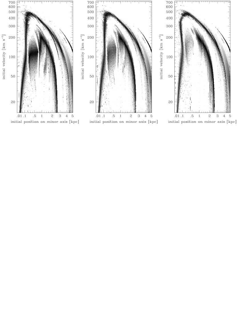
Figure 3: Ring-width diagrams in the Reference Model, as in the left-hand panel of Fig.1, but for the trajectories starting at the moments when the angle between the two bars is $\alpha=0.5\pi$ (left-hand panel), 0.4$\pi$ (central panel) and 0.2$\pi$ (right-hand panel). The diagrams are plotted as a function of the particle’s initial position along the minor axis of the outer bar, and of its initial value of velocity perpendicular to that axis.

As labels on the axes of the diagrams in Fig.1 indicate, we do not sample the phase-space of initial conditions uniformly, hence the volume of the phase-space $\Delta({\bf r},\dot{\bf r})$ corresponding to a given initial condition is

$$\Delta({\bf r},\dot{\bf r})=(\Delta y/r_{L})*(\Delta v/v_{\rm max}),$$ (3)

where $\Delta y$ is the local spacing in the sampling of the initial position on the minor axis, and $\Delta v$ is the local spacing in the sampling of the initial velocity. The volume $\Delta({\bf r},\dot{\bf r})$ of the phase-space element is normalized by the radius of the Lagrange point $L_{1}$ for the outer bar, $r_{L}$, and by $v_{\rm{max}}$. The histogram is constructed for 100 bins of the ring width, each covering equal fractional width (1 per cent) by adding the normalized volumes (3) grouped in bins determined by their ring width. Since we limit our search to particles remaining within the corotation of the outer bar, out of the 320,000 initial conditions sampled, we add to the bins only those, where the initial velocity is smaller than $v_{\rm{max}}$ for the given initial position on the minor axis (i.e. points located below the white line with black dots in the diagrams in Fig.1).

In Fig.2, the histogram for the single bar is drawn with the dotted line, and the solid line marks the histogram for the double bar. Starting from the left end, both histograms show a local peak at the normalized ring width of about 5 per cent. This peak corresponds to trajectories well trapped around the parent orbits – closed periodic orbits in a single bar and double-frequency orbits in double bars. The volume of phase-space occupied by trajectories mapping onto rings of width below 10 per cent is roughly the same in both histograms. This means that double-frequency orbits in double bars are equally good in trapping around themselves regular trajectories as closed periodic orbits are in single bars. But this is only true about closely trapped trajectories. The volume of phase-space occupied by trajectories that map onto rings of larger width, between 20 and 60 per cent, is systematically lower in double bars than it is in a single bar. This ’missing volume’ reappears in double bars at ring widths between 60 and 80 per cent as a separate component of the histogram. Its quasi-Gaussian shape indicates chaos, as we will confirm in Paper III. The absence of such a component in the histogram for a single bar indicates a much smaller fraction of chaotic motions there. A small fraction of chaotic orbits is indeed expected for a bar of relatively small axial ratio 2.5, and rather high Ferrers index of 2.

From the above analysis, we conclude that the amount of phase-space well trapped around double-frequency orbits in the Reference Model of a double bar and around closed periodic orbits in the corresponding model of a single bar is comparable, hence double-frequency orbits can provide the backbone for double bars in the same way as closed periodic orbits do in a single bar. On the other hand, the overall fraction of phase-space occupied by chaotic orbits in the model with double bars is much higher than in a single bar, which confirms the expectation that double bars introduce chaos. Note, however, that in our model, despite of large fractions of phase-space being chaotic, the regions of phase-space, where orbits forming the backbone of the system reside, remain largely regular.

3 Search for other regular orbits in the Reference Model

So far we considered only trajectories starting on the minor axis of the aligned bars, with the initial velocities perpendicular to that axis. This allowed us to recover double-frequency orbits in double bars that correspond to the x1 and x2 orbital families in a single bar. However, as we pointed out at the beginning of Section 2, the phase-space of initial conditions for trajectories in double bars has two more dimensions: the initial relative position angle of the bars and the initial radial velocity of the particle. Below, we extend our exploration of trajectories in double bars, so that the phase-space is sampled to a similar extent as with the surfaces of section in a single bar. This can be achieved by constructing two more types of 2-dimensional diagrams: one with a condition of aligned bars replaced by a given, non-zero initial relative position angle of the bars, and the second one by replacing the condition of zero initial radial velocity by a fixed angle between the initial velocity vector and the minor axis of two aligned bars.

3.1 Starting particles at various angles between the bars

In order to check whether the double-frequency orbits in the Reference Model trap around themselves a significant volume of regular orbits continuously, as the bars rotate with respect to each other, we calculated the ring widths for maps of trajectories that start at five more relative orientations of the bars. Each such map consists of points on trajectories recorded at that given relative orientation of the bars, and therefore it can indicate how the trapped trajectories behave as the bars rotate through each other.

We took as a reference the minor axis of the outer bar and, as before, we started particles from that axis, with the initial velocity perpendicular to it. We calculated the diagrams of ring widths for the initial angle between the bars equal to 0.2$\pi$, 0.4$\pi$, 0.5$\pi$, 0.6$\pi$ and 0.8$\pi$. Since the equation of motion is invariant with respect to time reversal, which reverses both the velocity of the particles and the rotation of the bars, trajectories launched when the angles between the bars are $\alpha$ and $\pi-\alpha$ are mirror images of one another, hence their diagrams of ring width are the same. In fact, our diagrams for $\alpha=0.2\pi$ and 0.8$\pi$ look the same, as well as the diagrams for 0.4$\pi$ and 0.6$\pi$, which makes a good consistency check. Thus, in Fig.3 we present only the diagrams for the relative angles of the bars $\alpha=0.5\pi$, 0.4$\pi$ and 0.2$\pi$.

The system is symmetric with respect to the axes of both bars only when the bars are aligned, or orthogonal. One may expect that in these two orientations trajectories starting orthogonally to the bar’s axes play a special role, as closed periodic orbits possessing this property do in a single bar. Thus the diagrams for bars aligned and orthogonal can be directly compared (left panels of Figs 1 and 3). In both diagrams one can see the two dark arches of similar shape and location, corresponding to the major orbital families. In both cases white stripes indicating irregular orbits run across them. The grey regions around the arches, marking regular trajectories trapped around double-frequency orbits, have similar extent in both diagrams, which means that a similar amount of initial conditions at bars aligned and orthogonal generates trapped trajectories. This observation can be quantified by comparing the histograms of ring widths for both diagrams, presented in Fig.4. Although the potential with two bars orthogonal has a slightly different Lagrange radius $r_{L}$, and $v_{\rm max}$ in (2) takes slightly different values, these differences are very small and they do not change the appearance of the histograms. The two histograms in Fig.4 look very similar, with the one for orthogonal bars having a slightly larger proportion of trajectories very well trapped (ring width about 5 per cent), and less irregular trajectories (ring widths above 60 per cent).

Figure 4: Histograms, as in Fig.2, of ring width for maps of trajectories in the Reference Model that start when the bars are aligned (solid line), and when they are orthogonal (dashed line).

For non-aligned or non-orthogonal bars, there is no symmetry of the system around any axis, but orbits dominated by one bar may still map onto loops that are symmetric about that bar’s axes. This is what we see in the diagrams for the angle between the bars equal to 0.4$\pi$ and 0.2$\pi$ (Fig.3, central and right panels). The outer arch represents orbits corresponding to the x1 orbits in a single bar, and probably dominated by that bar. The appearance of this arch is very similar in all three diagrams in Fig.3. The inner arch marks orbits corresponding to the x2 orbits in a single bar, but also forming the backbone of the inner bar in double bars (see MS00). This twofold nature of that family of orbits is reflected in Fig.3: the right leg of the arch, corresponding to the outer orbits, remains largely unchanged in all the three diagrams – these orbits are under the dominating influence of the outer bar. The left leg of the arch, corresponding to the inner orbits, gets increasingly pale as one moves to the diagrams for the angles $\alpha=0.4\pi$ and 0.2$\pi$, and it misses its darkest ’spine’. These orbits are dominated by the inner bar, and their maps are not symmetric around the outer bar’s minor axis, for which the diagrams were constructed. As the axes of the bars depart from each other, an increasing radial component in the initial velocity on these orbits is expected, which is not taken into account in constructing the diagrams in Fig.3. Thus for the angles $\alpha=0.4\pi$ and 0.2$\pi$, in the left ’leg’ of the lower arch, we likely see trajectories trapped around double-frequency orbits that themselves are not included in the diagrams.

It is interesting to point out that the division of the lower arch into the parts dominated by the inner and the outer bar coincides with the white stripe crossing that arch. This stripe means discontinuity in the orbital family, dividing it into two subfamilies: one following the inner, and one the outer bar. We did not find the source of the instability that this stripe represents, but it may play a crucial role in separating dynamically the inner bar from the rest of the system.

3.2 Trajectories with a radial component in the initial velocity

Thus far we considered only trajectories starting in the tangential direction, i.e. with no initial radial velocity component. In this subsection, we sample all other starting directions by constructing and analyzing a set of ring-width diagrams, each for a given angle $\theta$ between the initial velocity vector and the prograde tangential direction. The ring widths are measured for maps at the moments when the bars are aligned, and the trajectories start on the minor axis of the aligned bars.

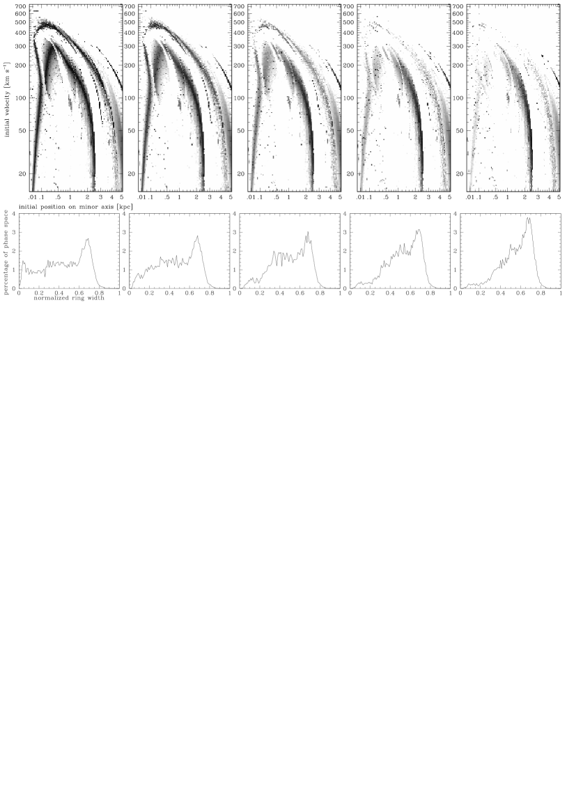
Figure 5: Top panels: Ring-width diagrams in the Reference Model, as in the left-hand panel of Fig.1, for the maps constructed when the bars are aligned, but for the initial velocity vector inclined to the prograde tangential direction at the angle (left to right diagrams): 0^∘, 3.6^∘, 7.2^∘, 10.8^∘ and 14.4^∘. Bottom panels: Corresponding histograms of the ring width.

3.2.1 Stability of double-frequency orbits to small radial velocity perturbation

The ring-width diagram from the left panel of Fig.1 already indicates that the two main families of double-frequency orbits in the Reference Model, represented by the two arches there, are stable with respect to small changes of the starting position on the minor axis of the aligned bars, and to small changes of the value of the initial prograde tangential velocity. In fact this stability is necessary in order to recover the double-frequency orbits from the ring-width diagrams, like the one in Fig.1. We still need to check, whether these double-frequency orbits remain stable when a small radial component in the initial velocity is added.

In order to confirm this, we calculated the ring widths for trajectories in the Reference Model as a function of three parameters: the starting position on the minor axis of the aligned bars, and the starting velocity (its value and direction), around the prograde tangential. With these three parameters one can describe all orbits that ever pass through the minor axis of the bars when the bars are aligned, and therefore obtain information equivalent to what surfaces of section give for a single bar. The calculated ring-widths constitute a data-cube, which can be displayed in the form of cuts for the constant direction of the initial velocity, as in the top panels of Fig.5. There, darkest arches, corresponding to smallest ring-widths, are found in the diagram for trajectories with no initial radial velocity (top-left panel). This means that the major double-frequency orbits have no radial velocity component when crossing the minor axis of the aligned bars. As the radial component of the initial velocity (i.e. the angle between the initial velocity vector and the prograde tangential direction) increases, the arches remain in place, although they gradually become brighter. This indicates that trajectories, whose initial conditions are the same as those of the major double-frequency orbits, except for a radial component in the initial velocity, remain trapped around those double-frequency orbits, as long as this radial component is sufficiently small. Trajectories with the initial velocity vector inclined to the prograde tangential direction at $\theta=3.6$^∘are trapped very well around the double-frequency orbits, but the trapping is much less efficient at $\theta=7.2$^∘. Interestingly, trajectories remain well trapped around the outermost x2 orbits (right leg of the inner arch) even at $\theta=14.4$^∘(Fig.5, top-right panel). Efficient trapping of trajectories proves that the major double-frequency orbits are stable to small radial velocity perturbations, and they can serve as the backbone for a doubly barred galaxy.

The lower panels of Fig.5 show the histograms of ring width. The first maximum, at the ring width of about 5 per cent, indicating trajectories very well trapped around double-frequency orbits, is notably absent in all histograms, except for the first one from the left, for which the initial radial velocity is zero. This again confirms that the major double-frequency orbits cross the minor axis of the aligned bars perpendicular to it. The characteristic quasi-Gaussian component on the right of each histogram, which indicates chaotic orbits, increases with the increasing radial component of the initial velocity. Overall, however, in all histograms from Fig.5, a considerable fraction of phase-space is still populated by regular orbits.

3.2.2 Exploration of all directions of the initial velocity vector

In the previous section, we explored trajectories with nearly prograde tangential initial velocity. Here we search for double-frequency orbits with a significant radial component of the initial velocity, hence we allow any initial velocity vector in the galactic plane. We still start the particle on the minor axis of the aligned bars. We construct a set of diagrams, each for a given angle $\theta$ between the initial velocity vector and the tangential prograde direction, plotting on the diagrams’ axes the position on the minor axis of the bars and the velocity value. The original diagram from Fig.1 was for $\theta=0$, and we constructed diagrams for $\theta=h\pi$, where $h$ runs from -1 to 1 in increments of 0.2.

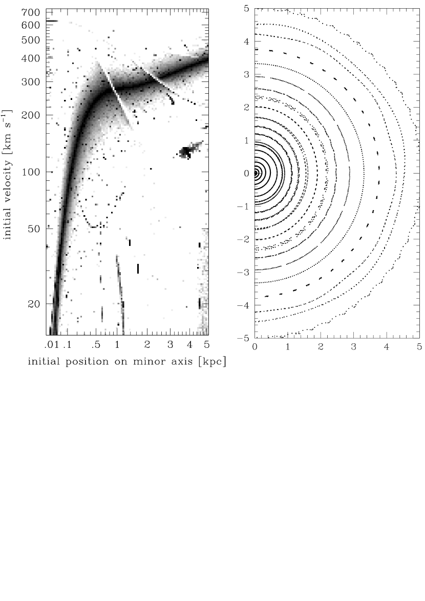
Figure 6: Left-hand panel: The ring-width diagram in the Reference Model, as in the left-hand panel of Fig.1, for the maps constructed when the bars are aligned, but for the initial velocity retrograde. Right-hand panel: Maps of trajectories well trapped around the retrograde double-frequency orbits (initial conditions taken from the darkest ’spine’ of the stripe in the left-hand panel), constructed at the moment when the angle between the bars is $\pi/4$ with the outer bar along the horizontal axis. Units on axes are in kpc.

In Sect.3.2.1, we showed that as $\theta$ departs from zero, the two arches in the top panels of Fig.5 gradually fade into grey, which indicates that there are regular trajectories with $\theta\neq 0$ still trapped around orbits for which $\theta=0$. Here we add that in the area covered by the arches from the top-left panel of Fig.5, most of the ring width remains below 50 per cent in the $\theta=\pm 0.2\pi$ diagrams, but in the $\theta=\pm 0.4\pi$ diagrams ring widths there are mostly above 50 per cent. This confirms that our sampling of $\theta$ is dense enough to recover double-frequency orbits that trap around themselves large regions of phase-space. The $\theta=\pm 0.6\pi$ diagrams are uniformly white – they contain no trajectories that map onto rings thinner than half of their radii, and certainly no double-frequency orbits capable of trapping around themselves any considerable volume of phase-space. The same is true for the $\theta=-0.8\pi$ diagram, while the $\theta=+0.8\pi$ diagram shows a very faint signature of orbits trapped around the inner orbits that manifest themselves in the $\theta=(\pm)\pi$ diagram.

The velocity vector for the $\theta=\pi$ diagram (Fig.6, left panel) is tangential retrograde, and, predictably, we recover regular trajectories trapped around the orbital family corresponding to the retrograde x4 family in a single bar (Contopoulos & Papayannopoulos 1980, see also Sellwood & Wilkinson 1993 for a review). Orbits from the darkest spine of the dark stripe in the diagram map onto loops, which are almost round and are shown in the right panel of Fig.6. We show the loops at the moment when the angle between the two bars is $\pi/4$, from which one can imply that the slightly elongated loops appear to be aligned with the inner bar at radii around 0.5 kpc, and with the outer bar at radii around 3 kpc. However, the highest ellipticity of the loops is only a few per cent, hence particles placed on these loops cannot recreate the density distribution as the bars rotate through each other. Since the loops do not oscillate much, the appearance of the ring-width diagram from the left-hand panel of Fig.6 remains the same if we repeat it for other relative angles of the bars, similarly to what we did in Sect.3.1 for prograde trajectories. Note that the diagram from Fig.6 appears smoother than that for the tangential prograde velocity from the left panel of Fig.1 – here it is disrupted by only two narrow white stripes marking irregular orbits, and otherwise it has a well defined ’spine’ with ring width increasing monotonically as one moves away from it.

This analysis shows that only parent orbits with the initial velocity tangential prograde (counterparts of the x1 and x2 orbits in a single bar) and retrograde (counterparts of the x4 family there) trap a significant volume of regular trajectories around themselves. The prograde trajectories remain trapped for larger range of angles between their initial velocity vector and the tangential direction than the retrograde trajectories do. The volume of phase-space occupied by the trapped orbits does not change significantly as the bars rotate through reach other (Sect.3.1).

4 Regular motions in 22 new models of double bars

Here we construct new models of double bars by varying parameters of the Reference Model in order to evaluate how the orbital support of double bars depends on the parameters of the system. Using the Reference Model as an example, we showed in the previous section that double-frequency orbits, which constitute the backbone of a doubly barred galaxy, originate from the x1 and x2 orbital families in a single bar. These double-frequency orbits can be found in maps of trajectories that cross the minor axis of the aligned bars tangentially (i.e. with no radial velocity). Such trajectories have only two free initial conditions: the initial position on the minor axis of the aligned bars and the initial tangential velocity, and we calculate here ring widths as a function of these two initial conditions only.

Table 1: Parameters of the models of double bars

Model		parameters of the
name		outer bar			inner bar
	$\rho_{c}$	$r_{L}$	$\frac{a_{1}}{b_{1}}$	$Q_{M}$	$\Omega_{2}$	$\frac{M_{2}}{M_{1}}$	$\frac{a_{2}}{a_{1}}$	$\frac{a_{2}}{b_{2}}$
01	4.8	6.0	2.5	4.5	110	0.15	0.2	2.0
02					80
03					90
04					100
05					120
06					110	0.11
07						0.13
08						0.17
09						0.19
10						0.15	0.16
11							0.18
12							0.22
13							0.24
14							0.2	1.5
15								2.5
16				2.25				2.0
17				9.0
18			2.0	4.5
19			3.0
20		5.5	2.5
21		6.5
22		7.0
23	2.4	6.0

$\rho_{c}$ is the central density in M_⊙kpc^-3 for the total mass distribution in the model, $r_{L}$ is the radial coordinate in kpc of the Lagrange point $L_{1}$ in the outer bar, $\frac{a_{1}}{b_{1}}$ is the axial ratio of the outer bar, $Q_{M}$ is the quadrupole moment of the outer bar in $10^{10}$ M_⊙kpc², $\Omega_{2}$ is the pattern speed of the inner bar in km s^-1 kpc^-1, $\frac{M_{2}}{M_{1}}$ is the mass ratio of the bars, $\frac{a_{2}}{a_{1}}$ is the ratio of the major axes of the two bars, $\frac{a_{2}}{b_{2}}$ is the axial ratio of the inner bar. Empty fields in the table indicate values the same as in the entry above.

In the simplest approach, each bar has at least 4 free parameters: size, mass, axial ratio and pattern speed. In the galaxy model there are also parameters of other components: the disk and the spheroid. This is a very big parameter space. We start its exploration by keeping the size of the outer bar unchanged, and by changing the other parameters one by one. In effect, we built 23 models, listed in Table 1, for which ring-width diagrams are presented in Fig.7, and histograms of ring width in Fig.8. In each model, volumes of phase-space, given by (3), that sum up to generate the histogram (see Sect.2.3), are normalized to the Lagrangian radius $r_{L}$ and the velocity $v_{\rm max}$ appropriate for that model. Below we analyze the models according to the parameters that were varied. Model 01 is our Reference Model.

Models with varying pattern speed of the inner bar, $\Omega_{2}$. We varied $\Omega_{2}$ between 80 and 120 km s^-1, with the Reference Model value being 110 km s^-1. Four models belonging to this group (02,03,04,05) are displayed in the left panels of the first row from the top in Fig.7, and their histograms – in the first panel from the left of the top row in Fig.8. From the histograms one can see that the slower the inner bar rotates, the higher is the fraction of phase-space occupied by chaotic orbits. This is reflected in the ring-width diagrams in Fig.7, where the disruption of both arches that mark the main families of orbits becomes more severe with decreasing pattern speed of the inner bar. In models 02 and 03, part of the outer arch is missing around the initial velocity about 400 km s^-1, hence there are no stable orbits to support the inner parts of the outer bar. In these same models, the white instability strip crossing the inner arch erases most of the stable orbits that were to support the inner bar. On the other hand, for pattern speeds higher than that in the Reference Model, the outer arch appears to be continuous, and the white stripe crossing the inner arch is much narrower, not disturbing much the orbital family supporting the inner bar. This exercise shows that double bars with the inner bar rotating faster than that in the Reference Model may be more dynamically plausible than that model.

Models with varying mass of the inner bar. We built four models, for which the mass of the outer bar is the same as in the Reference Model, while the mass ratio of the bars, $\frac{M_{2}}{M_{1}}$, varies between 0.11 and 0.19, with the Reference Model value being 0.15. Four models belonging to this group (06,07,08,09) are displayed in the left panels of the second row from the top in Fig.7, and their histograms – in the second panel from the left of the top row in Fig.8. Interestingly, varying the mass of the inner bar by almost a factor of 2 does not produce any noticeable difference in the extent of regular and chaotic zones in the system. Also ring-width diagrams have similar general appearance for all four models. However, a detailed look at these diagrams reveals that the upper arch becomes discontinuous at around 400 km s^-1 for the more massive inner bar. This again means a disruption of the inner orbits supporting the outer bar. Also the right leg of the outer arch is thinner for the more massive inner bar, which means that in general, the outer bar traps smaller volume of orbits once the inner bar becomes more massive. On the other hand, the white stripe crossing the inner arch becomes wider as the mass of the inner bar decreases, and it erases stable orbits supporting the inner bar. Therefore some intermediate mass of the inner bar, close to value assumed in the Reference Model, is adequate in the most regular system. We also note that the white stripe crossing the inner arch systematically moves to the right, with respect to that arch, as the mass of the inner bar increases.

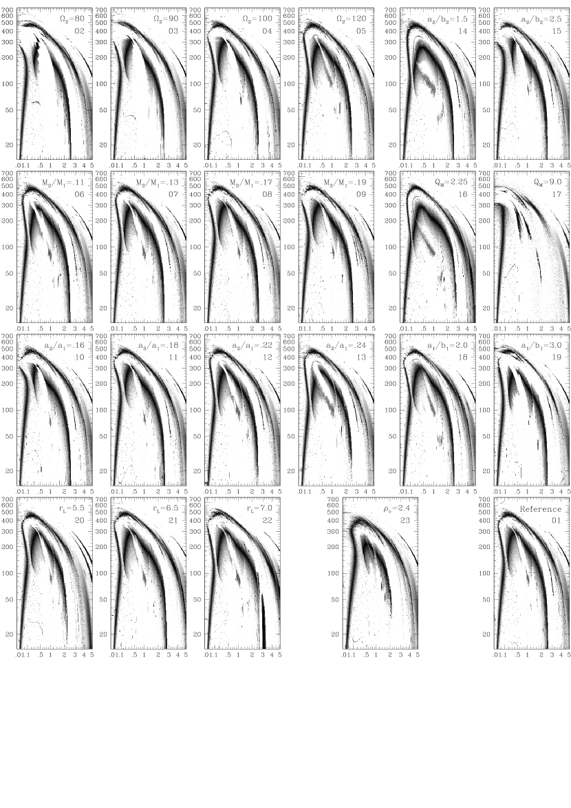
Figure 7: Ring-width diagrams, as in the left-hand panel of Fig.1, for the Reference Model (bottom-right corner) and 22 further models of doubly barred galaxies constructed in this work. The diagrams are gathered in groups, containing models for which one parameter is varied. The symbol of the varying parameter (explained in Table 1), together with its value, is given in the upper-right corner of each diagram, followed by the number of the model below it. As in the left panel of Fig.1, the coordinate along the horizontal axis of the diagrams is the initial position of the particle on the minor axis of the aligned bars, in kpc, and along the vertical axis – its initial tangential velocity in km s^-1.

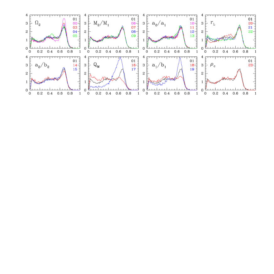
Figure 8: Histograms of ring width for the Reference Model (model 01) and the 22 new models. As in Fig.7, the histograms are gathered in groups: each plot displays a set of histograms for models, in which one parameter was varied. The varied parameter (explained in Table 1) is given in the upper-left corner of each plot. The models are colour-coded with their numbers listed in the plots in the appropriate colour. As in Fig.2, the coordinate along the horizontal axis of the histograms is the normalized ring width, and along the vertical axis – the percentage of phase-space.

Models with varying size of the inner bar. We built four models, for which the size of the outer bar is the same as in the Reference Model, while the size ratio of the bars, $\frac{a_{2}}{a_{1}}$, varies between 0.16 and 0.24, with the Reference Model value being 0.2. Four models belonging to this group (10,11,12,13) are displayed in the left panels of the third row from the top in Fig.7, and their histograms – in the third panel from the left of the top row in Fig.8. As in the case of varying the mass of the inner bar, there is no noticeable difference in the extent of regular and chaotic zones among the models. However, the ring-width diagrams show clear differences. In model 10, in which the inner bar is the smallest, the outer arch is again disrupted, around the initial velocity about 350 km s^-1. This is likely because we keep the mass of the inner bar constant between the 4 models considered here, and decreasing the size of the inner bar means increasing its density, which may lead to the disruption of orbits supporting the inner part of the outer bar. Making the inner bar larger for a given mass brings back the continuity of the outer arch, but then the stripe crossing the inner arch widens. In model 13, with the largest in size inner bar, a large fraction of that arch is being erased, weakening the backbone of the inner bar. As a result, some intermediate size of the inner bar, close to the value assumed in the Reference Model, is adequate in the most regular system, as it also is the case for the mass of the inner bar, which we found above. One other remark on this set of models is that even if the histograms of the models look the same, one can differentiate on the plausibility of these models based on their ring-width diagrams.

Models with varying axial ratio of the inner bar, $\frac{a_{2}}{b_{2}}$. We varied $\frac{a_{2}}{b_{2}}$ between 1.5 and 2.5, with the Reference Model value being 2.0. Two models belonging to this group (14,15) are displayed in the right panels of the first row from the top in Fig.7, and their histograms – in the first panel from the left of the bottom row in Fig.8. The differences between the histograms are small, but systematic: the smaller the axial ratio, the higher the volume of phase-space well trapped around the double-frequency orbits, and the smaller the fraction of the chaotic zones. This finding is confirmed by the ring-width diagrams. In the diagram for model 14 with the smallest axial ratio of the inner bar, the two arches are continuous, and there is even no white instability stripe crossing the inner arch. Thus the two main orbital families are continuously stable, providing good support for the two bars. This is not unexpected, given that the inner bar is closest to being axisymmetric in this model. To the contrary, in the diagram for model 15, with the biggest axial ratio of the inner bar, the two arches are discontinuous. This diagram shows that it may be difficult to construct models of double bars with a thin inner bar.

Models with varying mass of the outer bar. We built two models, for which the size of the outer bar is the same as in the Reference Model, while its quadrupole moment, $Q_{M}$, varies between $2.25\times 10^{10}$ M_⊙kpc² and $9.0\times 10^{10}$ M_⊙kpc². Since all other parameters of the bar remain unchanged, the quadrupole moment is proportional to the bar mass, and therefore there is a factor of 4 difference in the bar mass in our models. Two models belonging to this group (16,17) are displayed in the right panels of the second row from the top in Fig.7, and their histograms – in the second panel from the left of the bottom row in Fig.8. Both the histograms, and the the ring-width diagrams differ a lot. Model 17, with the most massive outer bar, shows a very large fraction of phase-space occupied by chaotic orbits, and the regular component of the histogram is scaled down. Its ring-width diagram shows only scattered fragments of the inner arch, and a very disrupted outer arch. This model is certainly prohibited dynamically, and we imply that it may be difficult to construct models of double bars with a very massive outer bar. On the other hand, the histogram for model 16, with the least massive outer bar, shows almost no chaotic component, and a good fraction of phase-space very well trapped around the parent orbits. The arches in its ring-width diagram are continuous. This model is preferred dynamically, but its outer bar is weaker than in the commonly observed double bars.

Models with varying axial ratio of the outer bar, $\frac{a_{1}}{b_{1}}$. We varied $\frac{a_{1}}{b_{1}}$ between 2.0 and 3.0, with the Reference Model value being 2.5. Two models belonging to this group (18,19) are displayed in the right panels of the third row from the top in Fig.7, and their histograms – in the third panel from the left of the bottom row in Fig.8. Unlike the similar change in the axial ratio of the inner bar, this change has clear consequences for the fractions of regular and chaotic zones in the system. In model 18, with the lowest axial ratio of the outer bar, the fraction of phase-space occupied by chaotic orbits is very small, while in model 19, with this axial ratio highest, the component of the histogram coming from the chaotic orbits dominates, while the regular component is scaled down. This is reflected in the ring-width diagrams. In model 19, the outer arch is very thin – a thin outer bar traps around itself trajectories confined to a very small volume of phase-space, and the inner arch is again disrupted by the white instability stripe. On the other hand, in model 18 both arches are continuous and thick enough to indicate good trapping of trajectories by the parent orbits. Like in the case of varying mass of the outer bar, we conclude that the model with small axial ratio of the outer bar is preferred dynamically, but such an outer bar is weaker than in the commonly observed double bars.

Models with varying radial coordinate of the Lagrange point $L_{1}$ of the outer bar, $r_{L}$. We varied $r_{L}$ between 5.5 and 7 kpc, with the Reference Model value being 6 kpc. The three models belonging to this group (20,21,22) are displayed in the left panels of the bottom row in Fig.7, and their histograms – in the right panel of the top row in Fig.8. The differences between the histograms are small, but systematic: the larger the $r_{L}$, the larger the volume occupied by trajectories well trapped around the double-frequency orbits, but also the higher the fraction of phase-space occupied by chaotic orbits. Thus histograms do not differentiate the models in terms of their dynamical plausibility. Moreover, the ring-width diagrams of the models look very similar. The only difference is seen in model 20, which loses orbital support for the outer part of the outer bar, since that bar’s semi-major axis is larger than its Lagrange radius. Trajectories in this part of model 20 remain regular, though, which is responsible for the diminution of low ring widths in its histogram, and a surplus of ring widths around 0.5. We conclude that the change of $r_{L}$ has little effect on the dynamical plausibility of the model.

Models with varying central density of the total mass distribution, $\rho_{c}$. In addition to varying the parameters of the bars, we varied $\rho_{c}$, which is likely to govern the extent of the orbital families. We constructed model 23 with $\rho_{c}$ twice smaller than in the Reference Model. It is displayed in the bottom row of Fig.7, and its histogram is in the right panel of the bottom row of Fig.8. Surprisingly, this histogram shows no considerable difference from the histogram of the Reference Model. On the other hand, the appearance of the ring-width diagrams is much different for these two models. In model 23, the outer arch is thicker, while the extent of the inner arch is much smaller. This is what one would expect from orbital structure in a single bar — for models with smaller central concentration, i.e. with smaller values of $\rho_{c}$, the extent of the x2 family is smaller (e.g. Athanassoula 1992a). Thus one would expect them to have a more pronounced x1 contribution and a less pronounced x2, as indeed our calculations show. Yet, we have explored only two models in the $\rho_{c}$ sequence and further work would be useful to understand better how this parameter affects the structure of double bars.

5 Discussion

5.1 Trends in the orbital response to changing parameters

In this paper, we explored a limited range of values for all essential parameters of double bars. We compared the ring-width diagrams and histograms of the models. Histograms clearly show a presence of a chaotic component, and they can be used to estimate the fraction of phase-space occupied by chaotic orbits. On the other hand, ring-width diagrams provide much more detailed information about which part of phase-space is affected by changing a given parameter of the model. A histogram provides information integrated over the ring-width diagram, and models with diverging structures in ring-width diagrams may produce very similar histograms. Models 01 and 23, for which the central mass density in the model was varied, illustrate this case. Although their histograms do not differ in any appreciable way, their ring-width diagrams are not at all alike, as they show different extents of the orbital families, and different volumes of the phase-space trapped around these families. Smaller extent of the x2 orbits in model 23 and smaller volume of phase-space trapped around the x1 family in model 01 result in almost identical integrated distribution in the histograms. Thus, it is worth stressing that the ring-width diagrams are much more sensitive indicators than the histograms. Nevertheless, the biggest differences among our models can already be seen in the histograms.

5.1.1 Size and mass

Clearly, the fraction of phase-space occupied by regular and chaotic orbits changes most, when the parameters of the outer bar are being varied (models 16–17, where $Q_{M}$ reflects the mass of the outer bar, and models 18–19, where the eccentricity of the outer bar is being varied). In models 16–17, this is partially because there are large changes of bar mass between the models — by a factor of 4. On the other hand, the axial ratio of the outer bar, varying only by a factor of 1.5 between models 18 and 19, brings spectacular differences between the ring-width diagrams, which can be witnessed clearly even in the histograms. The effect of varying these parameters on the onset of ergodicity is consistent with previous explorations of orbits in a single bar (e.g. Athanassoula et al. 1983): “more massive and/or more eccentric bars create more ergodicity”.

Among the parameters of the inner bar, its eccentricity has the same effect as for the outer bar — it increases the volume of chaotic motions. The orbital response to varying the next two parameters, the ratios of the masses and lengths of the bars, is not monotonic, as was the case for the parameters considered so far, and indicates the existence of optimum values. This is expected, because a too massive inner bar will destroy the outer bar, while an inner bar not massive enough cannot support itself. For a given mass of the inner bar, making this bar too small has the same effect as making it too massive for a given size. Although the histograms for these parameters do not differ significantly, the ring-width diagrams indicate the existence of such an optimum (Sect.4), and this optimum is very close to the parameters of the Reference Model. Therefore the Reference Model appears to be chosen optimally in terms of its mass and size.

The response of orbital support in double bars to the variation of the mass ratio of the bars was already studied by El-Zant & Shlosman (2003). They explored a two-dimensional surface in the phase-space of all possible initial conditions, span by the initial position on the major axis of the outer bar and the initial velocity perpendicular to that axis. We do the same in Sect.4, although our reference is the minor axis of the aligned bars, for reasons of continuity with previous work on periodic orbits. In this way, our study includes orbits self-intersecting on the major axis, which are common in strong bars (e.g. Athanassoula 1992a), while self-intersecting on, or near, the minor axis is rare. While for these initial conditions we calculate ring widths, El-Zant & Shlosman (2003) extract maximal extensions of a trajectory along the bar and normal to it, which quantifies whether this trajectory supports the bar. Both approaches indicate that when the inner bar is too massive in relation to the outer bar, orbits supporting the outer bar are disrupted, and that the inner bar cannot sustain its own orbital structure when it is not massive enough. We find the optimal mass ratio to be about 0.15, with 0.11 being probably too small, and 0.19 being rather too large. El-Zant & Shlosman (2003) find the ratio 0.01 being too small, the ratio 0.04 close to optimal, and the ratio 0.10 being already too large. The discrepancy of a factor of four in the optimal mass ratio arises most likely because El-Zant & Shlosman (2003) refer to a model of a doubly barred galaxy quite different from our Reference Model: the size ratio of the bars is 0.08 there, compared to our 0.20, and the ratio of pattern speeds is 8.3, while we adopt 3.1. From models 10–13 we see that a smaller inner bar should have a smaller optimal mass. We also note that the parameters of the El-Zant & Shlosman model correspond to a much weaker coupling between the bars than in our Reference Model.

5.1.2 Pattern speeds of the bars. Resonant coupling

Varying the Lagrangian radius of the outer bar (models 20–22) does not result in major changes of the orbital structure. It could be claimed that this is because we only explored values varying by a factor of 1.27. Nevertheless, this range is substantial since, at least for galaxies of type no later than SBc, reasonable values of the corotation radius of the bar can only be found in the range of 1.2$\pm$0.2 of its semi-major axis (Athanassoula 1992b).

Changing the pattern speed of the inner bar, $\Omega_{2}$ (models 02–05), causes significant changes in both histograms and ring-width diagrams, larger than the variations induced by changing the Lagrangian radius of the outer bar (models 20–22). The effect of varying $\Omega_{2}$ is significant, since that parameter changes only by a factor of 1.5 between the models. The fraction of the histogram occupied by chaotic orbits decreases with increasing $\Omega_{2}$, hence our models indicate that in order to minimize the contribution from chaotic motions, the corotation of the inner bar has to be brought as close as possible to the end of that bar. This result is contrary to what happens in a rapidly rotating single bar, where the region close to the corotation is associated with chaotic orbits, and therefore it increases contribution from chaotic motions. In our models, however, the inner bar extends to at most 60 per cent of its corotation radius (see Fig.9), hence it ends well within its ultraharmonic resonance, past which chaotic behaviour is expected in a bar.

Figure 9: Thick solid lines mark the angular velocity $\Omega$ (circular velocity divided by radius) in azimuthally averaged mass distribution of the Reference Model, and $\Omega-\kappa/2$, where $\kappa$ is the free oscillation frequency. Intersections of these curves with the dashed horizontal lines of constant pattern speeds of the bars (labeled by the model number, followed by the parameter that sets the bar’s pattern speed) define the corotation radii and the positions of the Inner Lindblad Resonances in the axisymmetric approximation. Two thin solid vertical lines, connecting to the upper and lower horizontal axes of the plot, mark the location of the Inner Lindblad Resonance of the outer bar (lower one) and the corotation radius of the inner bar (upper one) in the Reference Model. Thin dotted vertical lines mark the range of the Inner Lindblad Resonance of the outer bar and the corotation radius of the inner bar in models 02–05 and 20–22. The thick line segment on the lower horizontal axis indicates how far the corotation radius of the inner bar in the models above departs from the position of the Inner Lindblad Resonance of the outer bar in the Reference Model. The thick line segment on the upper horizontal axis indicates how far the position of the Inner Lindblad Resonance of the outer bar in the models above departs from the corotation radius of the inner bar in the Reference Model.

The reason why chaos is reduced in faster rotating inner bars is that for a corotation radius of the inner bar sufficiently small compared to the size of the outer bar, all resonances due to the inner bar fall in the part where the outer bar is nearly axisymmetric, i.e. the part where the force from the outer bar is near axisymmetric. This should decrease the amount of interaction between the two bars and thus also the amount of chaos. Therefore, a small corotation radius of the inner bar, i.e. a high $\Omega_{2}$, should reduce chaos, particularly in the inner part of the outer bar, in good agreement with what our calculations show. On the other hand, MS00 showed that in a doubly barred galaxy, an inner bar extending to its corotation has no orbital support. Therefore two opposing factors shape the ratio of the inner bar’s length to its corotation radius, and in the search for plausible models one should ensure that, in addition to maximizing the fraction of phase-space occupied by regular orbits, both bars are supported by loops throughout their extent. In Paper III, we will explore loops supporting the inner bar in models with various corotation radii, which will show whether the optimum should not be shifted in this respect.

The two bars in the Reference Model are roughly in resonant coupling: the azimuthally averaged Inner Lindblad Resonance of the outer bar is at 2.13 kpc, almost overlapping with the corotation radius of the inner bar at 2.19 kpc. Tagger et al. (1987) and Sygnet et al. (1988) proposed that resonant overlap enhances the coupling between nonlinear modes, even at reasonably low amplitudes. Such a coupling could also reduce the extent of chaotic zones in systems with multiple rotating patterns. In models 02–05 and 20–22, we varied pattern speed of each bar, which resulted in departures from resonant coupling. As shown in Fig.9, the position of the Inner Lindblad Resonance of the outer bar varies by factor 1.42 between 1.86 kpc in model 20 and 2.64 kpc in model 22, while the corotation radius of the inner bar varies by factor 1.45 between 2.01 kpc in model 05 and 2.92 kpc in model 02. Although departures from resonant coupling in our models are small, we do not see the expected minimization of chaos at resonant coupling. To the contrary, increasing $\Omega_{2}$ above the value set by resonant coupling results in an increase of regular motions in the system. This is in agreement with numerical simulations of nearly steady-state double bars (Rautiainen & Salo 1999; Shen & Debattista 2008; see Sect.5.2), which show no preference for resonant coupling between the bars.

From Fig.9 one can also notice that in the axisymmetric approximation, the $\Omega-\kappa/2$ curve intersects with the horizontal lines marking pattern speeds of the inner bar in models 02–04, which indicates the presence of an Inner Lindblad Resonance in the inner bar in these models. However, the ring-width diagrams do not indicate an additional orbital family associated with this resonance. This shows limitations of the axisymmetric approximation, already pointed out for a single bar, when the x2 orbits can be absent despite the presence of the azimuthally-averaged Inner Lindblad Resonance (e.g. Athanassoula 1992a).

5.2 Comparison with simulations of long-lasting double bars

Double bars are observed in a large fraction of barred galaxies – one third to one fourth according to Erwin & Sparke (2002) and Laine et al. (2002), which is consistent with them being being relatively long-lasting. If double bars last considerably longer than the time between their alignments, they can be approximated as oscillating systems. In this series of papers, we study the orbital support for the oscillating potential of double bars. Like the work on orbital structure in single bars, our models are not self-consistent, since we assume the potential in which we calculate the trajectories. A more complete picture of double bar dynamics should come from fully self-consistent N-body simulations of long-lasting double bars, for which our models can then provide orbital structure.

However, relating the orbital structure in oscillating potentials to numerical models is complicated by the fact that double bars which form in models including gas are often transient features: in the original models of Friedli & Martinet (1993), the decoupled bars survive no more than 7 alignments before they dissolve. In the simulation of Heller, Shlosman & Englmaier (2001) a gaseous ring, there referred to as a nuclear bar, tumbles retrograde in the outer bar’s frame for 9 alignments, before settling on a librating motion. When self-gravity of the gas is included, the ring-bar shrinks to the gravitational softening limit within 6 alignments of the bars (Englmaier & Shlosman 2004). All these modeled double bars, reviewed by Shlosman et al. (2005), are transient and comparing their time-dependent parameters with parameters of our models is not straightforward. Moreover, transient double bars cannot account for the large fraction of double bars observed at the present epoch.

More recent simulations of Heller, Shlosman & Athanassoula (2007a,b) show the longest-lasting double bars to date for models including a dissipative component. They use cosmological initial conditions, without any a priori assumptions on the parameters of the system. The inner bar survives there for at least 14 alignments of the bars, although it is far from steady-state: its amplitude decreases roughly three-fold during this time. The weakening of the inner bar can be caused by mass accumulation in the galaxy centre, following large radial inflow of gas reported by Heller et al. (2007a). Pfenniger & Norman (1990) find limit cycles or strange attractors enhancing the nuclear bar in their study of orbits of dissipative particles in double bars.

Long-lived double bars have been first reported in collisionless (stellar) systems by Rautiainen & Salo (1999). Their nuclear bars form first, survive several gigayears and rotate faster than the outer bars. Purely stellar double bars also formed in N-body models by Pfenniger (2001). More recently, Debattista & Shen (2007) and Shen & Debattista (2008) generated double bars in a purely stellar system. In their models, the inner bar forms from the bulge that is put in rotation by reversing velocities of particles with negative angular momenta. The inner bar lasts for 20 and more alignments, showing no decay in amplitude, hence it represents a true steady-state of the system.

Table 2: Parameters of double bars in models and numerical simulations

	Heller	Shen &	Reference	models
	et al.	Debattista	Model	02-23
$CR_{1}/a_{1}$	1.1–1.6	1.0–1.4	1.0	0.9–1.2
$CR_{2}/a_{2}$	5.0	3.25	1.83	1.5–2.5
$a_{2}/a_{1}$	.09–.14	.12–.19	.20	.16–.24
$\Omega_{2}/\Omega_{1}$	2.7	1.6–2.0	3.06	2.2–3.3
$CR_{1}/CR_{2}$	2.3	1.5–1.8	2.7	2.0–3.0

$CR_{1}$ and $CR_{2}$ are the corotation radii of the outer and the inner bar, respectively. The meaning of the other symbols is the same as in Table 1 and in the main text.

In Table 2, we compare the relative sizes of the bars and their rotation rates in our models with those extracted from the numerical simulations by Heller et al. (2007a) and Shen & Debattista (2008). The corotation of the outer bar, $CR_{1}$, in our models is given by its Lagrange radius, $r_{L}$. We use the values from the last, third phase of evolution of the Heller et al. (2007a) model, when the system is more stationary. Bars in the model by Shen & Debattista (2008, Model D) rotate with varying rate. We chose the $CR/a$ values in Table 2 for their minimal corotation radii, since there may be no orbital support for bars at higher radii.

As a single bar can extend almost to its corotation, MS00 tried to construct a model of double bars, in which also the inner bar extends to its corotation. Under the resonant coupling that they assumed (corotation of the inner bar on top of the Inner Lindblad Resonance of the outer bar), it turned out impossible: there were no orbits that could support the shape of the inner bar near its corotation. MS00 concluded that a self-consistent inner bar must end well inside of its own corotation. Now, the numerical simulations listed in Table 2 fully confirm this result: the $CR_{2}/a_{2}$ ratio there is even larger than in the Reference Model. This is because the Reference Model was constructed by MS00 in search for the largest possible inner bar. Its $a_{2}/a_{1}$ ratio is slightly larger than in the numerical models, and it is situated at the top end of the observed values (Erwin & Sparke 2002, Laine et al. 2002, Erwin 2004). A bar extending to its corotation radius incorporates higher-order orbital families (3:1, 4:1 etc.) that contribute to its shape. In a bar ending well within its corotation there is no such contribution. This suggests that the morphologies of the two bars in the dynamically possible double-barred systems should differ, while the implications from the observations are quite opposite: Erwin (2005) points out at many similarities between the inner and the outer bar in his images of doubly barred galaxies.

The ratio of pattern speeds (or corotation radii) in our models encompasses that in the Heller et al. model, but values in the Shen & Debattista model are somewhat lower. This may be a result of arbitrary initial conditions for the bulge, out of which the inner bar forms in that model. The ratio of the extent of the outer bar to its corotation radius consistently takes values around 1 in both simulations and in our models. Overall, the agreement between the parameters of our models and of double bars in numerical simulations indicates that the simulated systems are in fact supported by stable double-frequency orbits.

6 Conclusions

We conducted here an extensive survey of trajectories in a potential of double bars, with completeness similar to that of surfaces of section in a single bar. Using Model 2 from MS00 as our Reference Model, we found that only double-frequency orbits related to the fundamental x1, x2 and x4 orbits in a single bar trap around themselves the volume of regular orbits large enough to form the backbone of the double bar. Similar volumes of phase space are trapped around backbone orbits in single and double bars, hence the backbone of double bars appears as robust as in a single bar.

We also constructed 22 further models of double bars in order to study how the continuity of the fundamental x1 and x2 orbital families, and their ability to trap regular trajectories changes with varying the most essential parameters of the system. We found that the parameters of our Reference Model are optimal with those respects: the inner bar has an optimal size for its given mass and vice versa. Otherwise, increasing the eccentricity of the inner bar increases the fraction of phase-space occupied by irregular orbits, as is already known for the outer bar.

The ratio of inner bar’s size to its corotation radius must be such that there are orbits supporting the inner bar throughout its extent, but also such that chaotic zones, breaking the continuity of orbital families, are not too large. Since one condition requires a small ratio, while the other, a large one, only when these two conditions can be reconciled, the double bar is dynamically possible. There is no obvious relation of the conditions above to the postulated resonant coupling between the bars. In fact, we observe reduced chaos in a model that departs from resonant coupling, which indicates that resonant coupling may not minimize chaos in double bars.

Recent numerical simulations produced double bars that last long enough to implicate underlying periodicity in the potential, thus making it possible to test predictions of the orbital analysis. The main prediction of MS00, that the inner bar should end well within its corotation is fully confirmed by these simulations, which reinforces the predictive power of orbital studies. Moreover, in the simulated bars, the corotation radius of the inner bar can be as far as five times its extent. This calls for extending the analysis presented here to finding orbital support of the simulated systems.

Acknowledgments. This work was supported by the Polish Committee for Scientific Research as a research project 1 P03D 007 26 in the years 2004–2007 (WM), and by the grant ANR-06-BLAN-0172 in the years 2006–2007 (EA). It was in part carried out within the framework of the European Associated Laboratory “Astrophysics Poland-France”.

References

- (1) Athanassoula E., Bienayme O., Martinet L., Pfenniger D., 1983, A&A, 127, 349
- (2) Athanassoula E., 1992a, MNRAS, 259, 328
- (3) Athanassoula E., 1992b, MNRAS, 259, 345
- (4) Contopoulos G., Papayannopoulos Th., 1980, A&A, 92, 33
- (5) Debattista V.P., Shen J., 2007, ApJ, 654, L127
- (6) El Zant A., Shlosman I., 2003, ApJL, 595, L41
- (7) Englmaier P., Shlosman I., 2004, ApJL, 617, L115
- (8) Erwin P., Sparke L.S., 2002, AJ, 124, 65
- (9) Erwin P., 2004, A&A, 415, 941
- (10) Erwin P., 2005, MNRAS, 364, 283
- (11) Friedli D., Martinet L., 1993, A&A, 277, 27
- (12) Heller C., Shlosman I., Athanssoula E., 2007a, ApJ, 657, L65
- (13) Heller C., Shlosman I., Athanssoula E., 2007b, ApJ, 671, 226
- (14) Heller C., Shlosman I., Englmaier P., 2001, ApJ, 553, 661
- (15) Laine S., Shlosman I., Knapen J.H., Peletier R.F., 2002, ApJ, 567, 97
- (16) Lichtenberg A.J., Lieberman M.A., 1992, Regular and Chaotic Dynamics, 2nd edition. Springer, New York
- (17) Louis P.D., Gerhard O.E., 1988, MNRAS, 233, 337
- (18) Maciejewski W., Sparke L.S., 1997, ApJL, 484, L117
- (19) Maciejewski W., Sparke L.S., 2000, MNRAS, 313, 745 (MS00)
- (20) Maciejewski W., Athanassoula E., 2007, MNRAS, 380, 999 (Paper I)
- (21) Pfenniger D., Norman C., 1990, ApJ, 363, 391
- (22) Pfenniger D., 2001, in: Hibbard J.E., Rupen M., van Gorkom J.H. (eds.) ASP Conf. Ser. Vol. 240, Gas and Galaxy Evolution. Astron. Soc. Pac. San Francisco, p.319
- (23) Rautiainen P., Salo H., 1999, A&A, 348, 737
- (24) Sellwood J.A., Wilkinson A., 1993, Rep. Prog. Phys., 56, 173
- (25) Shen J., Debattista V.P., 2008, ApJ, submitted (arXiv:0711.0966)
- (26) Shlosman I., 2005, in: Huettemeister S., Manthey E. (eds.) The Evolution of Starbursts, AIP, Melville, 223
- (27) Sygnet J.F., Tagger M., Athanassoula E., Pellat R., 1988, MNRAS, 232, 733
- (28) Tagger M., Sygnet J.F., Athanassoula E., Pellat R., 1987, ApJ, 318, L43