Karhunen-Loève Basis Functions of Kolmogorov Turbulence in the Sphere

Abstract

The statistically independent Karhunen-Loève modes of refractive indices with isotropic Kolmogorov spectrum of the covariance are calculated inside a sphere of given radius, rendered as series of 3D Zernike functions. Many of the symmetry arguments of the associated 2D problem for the circular input pupil remain valid. The technique of efficient diagonalization of the eigenvalue problem in wavenumber space is founded on the Fourier representation of the 3D Zernike basis.

I Overview

I.1 Model of the Refractive Index Structure Function

This paper describes modeling of variations of refractive indices $n$ based on their structure functions $\mathcal{D}$

$$\mathcal{D}_{n}(\Delta\mathbf{r})=C_{n}^{2}|\Delta\mathbf{r}|^{\gamma}$$ (1)

with Kolmogorov power index

$$\gamma=2/3,$$ (2)

sampled at points which are $\Delta\mathbf{r}$ apart and located in an air volume between the light source and some input pupil of a receiver. The familiar assumptions of this model are

• “single layer” homogeneity: the refractive index structure constant $C_{n}^{2}$ is indeed constant over the entire volume that is probed by the electromagnetic wave,

• isotropy: the structure function depends on the absolute value of the vector $\Delta\mathbf{r}$, but not on its direction.

In the conjugated Fourier variable $\bm{f}$ of wave numbers, the turbulent spectrum is represented by the (again isotropic) Wiener spectrum $\Phi_{n}(f)$ Noll (1976); Pérez and Zunino (2008). The expectation value of the mean appears as a constant in the Fourier kernel, and the expectation value of the covariance as a cosine:

$$\mathcal{D}_{n}(\Delta\mathbf{r})=2\int\Phi_{n}(f)[1-\cos(2\pi\bm{f}\cdot\Delta\mathbf{r})]d^{3}f.$$ (3)

[The imaginary part of the factor $\exp(2\pi i\bm{f}\cdot\Delta\bm{r})$, which is induced by the shift theorem Fourier transforms and which represents the contributions with odd parity, vanishes by isotropy after integration.] The power spectrum is Conan (2008, 2000)

$$\Phi_{n}(f)=-\pi^{3/2-\beta}\frac{\Gamma(\beta/2)}{2\Gamma(\frac{3-\beta}{2})}C_{n}^{2}f^{-\beta}\equiv c_{\Phi}C_{n}^{2}f^{-11/3};\quad c_{\Phi}\approx 0.00969315,$$ (4)

at a power spectral index

$$\beta=\gamma+3\quad(=11/3).$$ (5)

Where the variable $\bm{\kappa}=2\pi\bm{f}$ is used in lieu of $\bm{f}$, the constant $(2\pi)^{\gamma}c_{\Phi}\approx 0.033005$ takes the role of $c_{\Phi}$.

I.2 Circular (Projected) 2D Case

Above, the structure function and its spectrum are defined as functions of the 3D distances $\Delta r$ and $\sigma$. Integration along two parallel lines of sight through a layer of vertical thickness $h$ at an air mass $1/\sin a$ at a projected baseline $P$ for momentum number $k$ (equal to $2\pi$ divided through the wavelength of the electromagnetic wave) defines 2D phase structure functions

$$\mathcal{D}_{\varphi}(P)=C_{n}^{2}k^{2}g(\gamma)P^{\gamma+1}\frac{h}{\sin a},$$ (6)

where

$$g(\gamma)=\sqrt{\pi}\frac{\Gamma(-(1+\gamma)/2)}{\Gamma(-\gamma/2)}\approx 2.9144,\quad(\gamma=2/3)$$ (7)

is a geometric constant from the integration Roddier (1981); Fried (1965); Hufnagel and Stanley (1964); Strohbein (1971). The information sampled along the pencils of length $h/\sin a$ through the layer is reduced to $\mathcal{D}_{\varphi}$, a function of the two components of $P$ in the input pupil of the receiver. Noll’s notation $\Phi_{\varphi}(\nu)=0.023r_{0}^{-5/3}\nu^{-11/3}$ of the associated 2D power spectrum of the phase differences in terms of the Fried parameter $r_{0}$—at the wavelength $2\pi/k$ of the electromagnetic spectrum— (Noll, 1976, (21)) is equivalent as we note that $0.023$ is the product of the ad-hoc scaling parameter Fried (1966a)

$$2[(24/5)\Gamma(6/5)]^{5/6}\approx 6.883877$$ (8)

by

$$-\frac{\Gamma(\beta/2)}{2\pi^{2+\gamma}\Gamma(1-\beta/2)}\approx 0.0033260.$$ (9)

The association of the constants in equations (4), (7) and (9) is summarized in the following diagram. The role of $g(\gamma)$ switches from multiplier to divisor while transiting from real to wavenumber space.

The intend is to show how the phase structure function is associated with integration of a refractive index structure function over path lengths; the Fried parameter and some of the associated geometric constants will disappear from the analysis of the next section, where no such path integration is performed.

This concludes the overview of the literature. Karhunen-Loève (KL) modes in the projected (2D) case are not reviewed here; we refer to the available literature Fried (1978); Dai (1995); Roddier (1990); Mathar (2007a).

I.3 Applications

The aim of calculations in section II is to remove the constraint of working with optical path lengths integrated along two thin, parallel rays through the turbulent atmosphere. Simulations of anisoplanatism, multi-conjugate adaptive optics, and atmospheric transfer functions for radio (as opposed to optical) receivers often integrate over extended fields-of-view. Essentially we factorize the problem; we provide means to fill a volume with instances of a turbulent refractive index, but keep aside by which weighing scheme sub-volumes accumulate the instrumental signal.

To keep mathematics simple, this volume is given spherical shape, the shape that is symmetry-adapted to the isotropy of the structure function. As one extreme application of the geometry one could image the center of this sphere at the center of the Earth, the sphere radius set to the Earth radius plus some tenth of kilometers, and then evaluating refractive indices only in the thin inner hull close to the sphere surface—representing the entire Earth’s atmosphere—computed from superposition of the KL modes.

II Karhunen-Loève Functions in the Sphere

II.1 Spherical Basis

The generic form of the Karhunen-Loève eigenvalue equation for the modes $K$ and their eigenvalues ${\cal B}^{2}$ associated with a covariance $C$ sampled over a spherical region of radius $R$ is

$$\int_{r^{\prime}\leq R}C(|\mathbf{r}-\mathbf{r}^{\prime}|)K(\bm{r^{\prime}})d^{3}r^{\prime}={\cal B}^{2}K(\bm{r}).$$ (10)

One benefit earned from the constraints of the model described in section I.1 is that a radial scaling

$$r=Rx$$ (11)

maps these cases onto a single unified model inside the unit sphere:

$$\int_{x^{\prime}\leq 1}|\mathbf{x}-\mathbf{x}^{\prime}|^{\gamma}K(\mathbf{x^{\prime}})d^{3}x^{\prime}=\frac{{\cal B}^{2}}{C_{n}^{2}R^{\gamma+3}}K(\mathbf{x}).$$ (12)

The other benefit is that the spherical symmetry of the domain of integration matches the isotropy in the covariance; moving on to the Fourier domain of the dimensionless $\bm{\sigma}=R\bm{f}$,

$$K(x^{\prime})=\int d^{3}\sigma K(\bm{\sigma})e^{-2\pi i\bm{\sigma}\cdot\mathbf{x^{\prime}}}$$ (13)

and

$$C(|x-x^{\prime}|)=\int d^{3}\sigma C(\sigma)e^{-2\pi i\bm{\sigma}\cdot(\mathbf{x}-\mathbf{x}^{\prime})}$$ (14)

transforms the convolution into a product, in which the eigenvalue problem is block diagonal in the angular variables Roddier (1990),

$$C(\sigma)K({\bf\sigma})=\frac{{\cal B}^{2}}{R^{\gamma+3}}K(\sigma).$$ (15)

With the same argument as for the 2D case, ie, because the exponent of $C\propto\sigma^{-\beta}$ is too large for the Kolmogorov spectrum to remain integrable in the large-scale limit $\sigma\to 0$, the decomposition (15) is not possible for functions with nonzero $K(\sigma)$ at the origin of the $\sigma$-space: the homogeneous mode, the analog to the 2D piston mode, is left out of the analysis. ${\cal D}_{n}$ does not convey information on the mean of the refractive index.

II.2 Diagonalization in Wavenumber Space

Subject to the usual ambiguity of any choice of basis functions, we expand the $K(x)$ in an orthogonal Zernike basis, suggested in Appendix A, serializing the eigenfunctions for each block $l$ of the eigenvalue problem by an index $p$:

$$K_{p}^{(l)}(\bm{\sigma})=\sum_{n}\kappa_{n,l,p}Z_{nl}^{(m)}(\bm{\sigma})=4\pi\sum_{n}\kappa_{n,l,p}i^{l}Y_{l}^{m}(\theta_{\sigma},\phi_{\sigma})R_{n}^{(l)}(\sigma).$$ (16)

The reduction of (15) with (4) reads

$$c_{\Phi}\sigma^{-\beta}K_{p}^{(l)}(\sigma)=\lambda_{p,l}^{2}K_{p}^{(l)}(\sigma);\quad\lambda_{p,l}^{2}=\frac{{\cal B}^{2}}{R^{\beta}C_{n}^{2}}.$$ (17)

Formulation of an eigenvalue problem of matrix algebra proceeds with (40),

$$c_{\Phi}\sum_{n}\kappa_{n,l,p}\int_{0}^{\infty}\sigma^{2}\sigma^{-\beta}R_{n}^{(l)}(\sigma)R_{n^{\prime}}^{(l)}(\sigma)d\sigma=\frac{\lambda_{p,l}^{2}}{(4\pi)^{2}}\kappa_{n^{\prime},l,p}$$ (18)

A core integral matrix $I_{n,n^{\prime}}^{(l)}$ is defined to tighten the notation,

$$c_{\Phi}\int_{0}^{\infty}\sigma^{2}\sigma^{-\beta}R_{n}^{(l)}(\sigma)R_{n^{\prime}}^{(l)}(\sigma)d\sigma\equiv I_{nn^{\prime}}^{(l)}\frac{1}{(4\pi)^{2}}.$$ (19)

The integral over the product of Bessel Functions of the form (39) yields (Gradstein and Ryshik, 1981, 6.574.2)(Magnus and Oberhettinger, 1948, p. 49)

$$I_{nn^{\prime}}^{(l)}=c_{\Phi}\frac{\pi^{\beta}}{2}\sqrt{(2n+3)(2n^{\prime}+3)}(-1)^{(n-n^{\prime})/2}\frac{\Gamma(\beta+1)\Gamma(\frac{n+n^{\prime}+3-\beta}{2})}{\Gamma(\frac{n-n^{\prime}+\beta}{2}+1)\Gamma(\frac{n^{\prime}+n+\beta+5}{2})\Gamma(\frac{n^{\prime}-n+\beta}{2}+1)}$$ (20)

for $n,n^{\prime}=l,l+2,l+4,\ldots$. These are the matrices to be diagonalized to establish the KL basis functions, one matrix for each $l$,

$$\sum_{n}I_{n,n^{\prime}}^{(l)}\kappa_{n,l,p}=\lambda_{p,l}^{2}\kappa_{n^{\prime},l,p}.$$ (21)

The upper right corners of the symmetric $I_{n,n^{\prime}}^{(l)}=I_{n^{\prime},n}^{(l)}$ are shown in Table 1 for even and in Table 2 for odd $l$. The individual array for a specific $l$ is the sub-array in which all rows $n<l$ and columns $n^{\prime}<l$ are removed. A common factor has been split off to write them as exact fractions. If no such scaling is chosen, tables like Table 3 result. As argued at the end of section II.1, row $n=0$ and column $n^{\prime}=0$ in Table 1 are deleted prior to the diagonalization.

Table 1: $I_{nn^{\prime}}^{(l)}/[2^{2/3}\pi\sqrt{(2n+3)(2n^{\prime}+3)}]$ for $n,n^{\prime}\leq 12$, $l$ even. Multiply by $\sqrt{(2n+3)(2n^{\prime}+3)}$ and in addition by $2^{2/3}\pi\approx 4.986967$ to obtain $I_{nn^{\prime}}^{(l)}$. The table is symmetric; only the non-redundant upper right triangle is shown.

	0	2	4	6	8	10	12
0	$-{\frac{54}{385}}$	$-{\frac{54}{7735}}$	${\frac{27}{142324}}$	${\frac{135}{78420524}}$	${\frac{27}{215656441}}$	${\frac{27}{1545789175}}$	${\frac{27}{7647588550}}$
2		${\frac{27}{20020}}$	$-{\frac{27}{117572}}$	${\frac{135}{7436429}}$	${\frac{27}{98025655}}$	${\frac{27}{980256550}}$	${\frac{27}{5637584050}}$
4			${\frac{27}{209209}}$	$-{\frac{27}{734825}}$	${\frac{27}{6760390}}$	${\frac{27}{357505330}}$	${\frac{27}{3038795305}}$
6				${\frac{27}{950950}}$	$-{\frac{27}{2679950}}$	${\frac{27}{20957209}}$	${\frac{27}{977699359}}$
8					${\frac{27}{2947945}}$	$-{\frac{621}{168568855}}$	${\frac{27}{51867340}}$
10						${\frac{621}{167806100}}$	$-{\frac{18009}{11151478100}}$
12							${\frac{3132}{1803915575}}$

Table 2: $I_{nn^{\prime}}^{(l)}/[2^{2/3}\pi\sqrt{(2n+3)(2n^{\prime}+3)}]$ for $n,n^{\prime}\leq 13$, $l$ odd.

	1	3	5	7	9	11	13
1	${\frac{54}{5005}}$	$-{\frac{27}{30940}}$	${\frac{135}{2704156}}$	${\frac{135}{215656441}}$	${\frac{27}{490128275}}$	${\frac{27}{3091578350}}$	${\frac{27}{13945602650}}$
3		${\frac{27}{76076}}$	$-{\frac{27}{323323}}$	${\frac{27}{3380195}}$	${\frac{27}{196051310}}$	${\frac{27}{1787526650}}$	${\frac{27}{9583892885}}$
5			${\frac{27}{475475}}$	$-{\frac{27}{1469650}}$	${\frac{27}{12327770}}$	${\frac{27}{607759061}}$	${\frac{27}{4888496795}}$
7				${\frac{459}{29479450}}$	$-{\frac{27}{4555915}}$	${\frac{27}{33713771}}$	${\frac{27}{1504152860}}$
9					${\frac{621}{109073965}}$	$-{\frac{621}{259336700}}$	${\frac{783}{2230295620}}$
11						${\frac{18009}{7215662300}}$	$-{\frac{3132}{2787869525}}$
13							${\frac{3132}{2525481805}}$

Table 3: $I_{nn^{\prime}}^{(1)}$ limited to $n,n^{\prime}\leq 11$. This repeats the values of Table 2 without the scale factor.

	$1$	$3$	$5$	$7$	$9$	$11$
1	$0.269027$	$-0.029194$	$0.002007$	$0.000029$	$0.000003$	$0.000000$
3		$0.015929$	$-0.004505$	$0.000493$	$0.000009$	$0.000001$
5			$0.003681$	$-0.001362$	$0.000180$	$0.000004$
7				$0.001320$	$-0.000558$	$0.000082$
9					$0.000596$	$-0.000274$
11						$0.000311$

As already in the 2D case, the relative strength of values on the diagonals compared to the sub-diagonals is predictive of how close the KL modes resemble pure Zernike functions. An explicit table of the dominant modes is given in Appendix B, sorted with respect to decreasing $\lambda_{p,l}^{2}$.

II.3 Real-valued Basis

In practice, the component $e^{im\phi}$ of the spherical harmonics in the Zernike basis (25) may be replaced by switching in the real-valued functions Bradley and Cracknell (1972)

$$\sqrt{\epsilon_{m}}\cos(m\theta),\quad\sqrt{\epsilon_{m}}\sin(m\theta),$$ (22)

where

$$\epsilon_{m}\equiv\left\{\begin{array}[]{ll}1,&m=0\\ 2,&m\geq 1\end{array}\right.$$ (23)

is the Neumann factor. This choice maintains normalizations, and maintains the $2l+1$ fold degeneracy of the Karhunen-Loève modes.

III Summary

This work traced the well-known Karhunen-Loève functions of a covariance with power spectral index 5/3 over a circular telescope entrance pupil back to the associated functions with power spectral index 2/3 over the sphere. The solution of the eigenvalue integral equation for the covariance has been formulated for expansions in a 3D Zernike basis. Bare Zernike functions turn out to be good approximations to the large scale modes.

Appendix A 3D Zernike Basis

A.1 Definition

We define an orthogonal 3D Zernike Basis $Z_{n,l}^{(m)}(r,\theta,\phi)$ over the unit sphere in strict analogy to the domain of the unit circle Bhatia and Wolf (1954, 1952) as a product over (i) Courant-Hilbert Jacobi polynomials $G$ to span the radial coordinate $x$ and (ii) Spherical Harmonics $Y_{l}^{m}$ to cover the azimuthal and polar angles $\phi$ and $\theta$:

$$Z_{n,l}^{(m)}\equiv R_{n}^{(l)}(x)Y_{l}^{m}(\theta,\phi),\quad 0\leq x\leq 1,\quad 0\leq\theta\leq\pi,\quad 0\leq\phi\leq 2\pi.$$ (24)

Spherical Harmonics

$$Y_{l}^{m}=\sqrt{\frac{(2l+1)(l-|m|)!}{4\pi(l+|m|)!}}P_{l}^{|m|}(\cos\theta)e^{im\phi},\quad-l\leq m\leq l,$$ (25)

are a product of $e^{im\phi}\sin^{|m|}\theta$ with a polynomial in $\cos\theta$ of degree $l-|m|$. (There are at least three different sign/phase conventions in the literature, of which only one is picked by this equation. Since the manuscript does not deal with aspects of angular momentum coupling, the specific choice is not relevant.) The transformation to Cartesian coordinates $(x\sin\theta\cos\phi,x\sin\theta\sin\phi,x\cos\theta)$ has been discussed in the literature Mathar (2002); Novotni and Klein (2004).

Rotation of the 3D coordinate system mixes the components of $Y_{l}^{m}$, keeping $l$ constant (Bradley and Cracknell, 1972, 2.1.3)Altmann (1957); Edmonds (1957). The role of the azimuthal number $m$ of the 2D case Noll (1976) is therefore taken over by $l$ to set the lowest order to the radial polynomials Bhatia and Wolf (1954); Novotni and Klein (2003, 2004). With this constraint, demanding orthogonality with respect to the weight function $x^{2}$ in $0\leq x\leq 1$ (of the Jacobian of the spherical coordinates), and setting a smoothness-constraint at the origin $x=0$ in the sense that the powers of $x$ in the polynomial are all either even or odd, the radial functions need to be proportional to $x^{l}G_{\alpha}(q,q,x^{2})$, where

$$G_{\alpha}(q,q,y) = \frac{\Gamma(q+\alpha)}{\Gamma(q+2\alpha)}\sum_{k=0}^{\alpha}(-1)^{k}{\alpha\choose k}\frac{\Gamma(q+2\alpha-k)}{\Gamma(q+\alpha-k)}y^{\alpha-k}$$ (26)

$$= \frac{\Gamma(q+\alpha)}{\Gamma(q+2\alpha)}(-1)^{\alpha}\sum_{k=0}^{\alpha}\frac{\Gamma(\alpha+1)}{\Gamma(\alpha-k+1)k!}\frac{\Gamma(q+\alpha+k)}{\Gamma(q+k)}(-y)^{k}$$ (27)

$$= \frac{\Gamma^{2}(q+\alpha)}{\Gamma(q+2\alpha)\Gamma(q)}(-1)^{\alpha}\,_{2}F_{1}(-\alpha,q+\alpha;q;y)=(-1)^{\alpha}\frac{{q+\alpha-1\choose\alpha}}{{q+2\alpha-1\choose\alpha}}\,_{2}F_{1}(-\alpha,q+\alpha;q;y)$$ (28)

are Courant-Hilbert Jacobi polynomials (Abramowitz and Stegun, 1972, 22.3.3) with parameters

$$\alpha\equiv(n-l)/2,\quad q\equiv l+3/2.$$ (29)

The characteristic difference with the 2D case, see Mathar (2007b) and references therein, is that the parameter $q$ has increased by $1/2$ to cope with the higher power of the Jacobian of the Cartesian-to-spherical (as opposed to Cartesian-to-circular) transformation of coordinates. [This boost of the parameter remains visible in the matrix elements (20) and remains visible in the Bessel Function indices (39) which are translated from integer to half-integer values.] Ortho-normalization based on their orthogonality (Abramowitz and Stegun, 1972, 22.2.2) yields

$$R_{n}^{(l)}(x) \equiv \sqrt{2n+3}\frac{\left(\frac{n+l}{2}+1\right)!(2n+2)!}{2^{n-l}(n+l+2)!\left(\frac{n-l}{2}\right)!(n+1)!}x^{l}G_{(n-l)/2}(l+\frac{3}{2},l+\frac{3}{2},x^{2})$$ (30)

$$= \sqrt{2n+3}\frac{\Gamma(2\alpha+q)}{\Gamma(\alpha+q)\Gamma(\alpha+1)}x^{l}G_{\alpha}(q,q,x^{2}),$$ (31)

$$\int_{0}^{1}x^{2}R_{n}^{(l)}(x)R_{n^{\prime}}^{(l)}(x)dx=\delta_{n,n^{\prime}}.$$ (32)

Some examples of these polynomials are given in Table 4 for comparison with the 2D case (Noll, 1976, Table I). A subset is also visualized in Figure 1 for comparison with (Mak et al., 2008, Fig. 1). The nodal counts are as expected for any of the classical orthogonal polynomials. The overall choice of signs, ie, $R_{n}^{(l)}(1)>0$, is just inherited from the Jacobi polynomials, and carries no physical significance.

Table 4: The radial polynomials $R_{n}^{(l)}(x)$ for $l\leq 4$ and $n\leq 10$.

$l$	$n$	$R_{n}^{(l)}(x)$
0	0	$\sqrt{3}$
0	2	$\frac{1}{2}\sqrt{7}\left(-3+5\,{x}^{2}\right)$
0	4	$\frac{1}{8}\sqrt{11}\left(15+63\,{x}^{4}-70\,{x}^{2}\right)$
0	6	$\frac{1}{16}\sqrt{15}\left(-35+429\,{x}^{6}-693\,{x}^{4}+315\,{x}^{2}\right)$
0	8	${\frac{1}{128}}\,\sqrt{19}\left(315+12155\,{x}^{8}-25740\,{x}^{6}+18018\,{x}^{4}-4620\,{x}^{2}\right)$
0	10	${\frac{1}{256}}\,\sqrt{23}\left(-693+88179\,{x}^{10}-230945\,{x}^{8}+218790\,{x}^{6}-90090\,{x}^{4}+15015\,{x}^{2}\right)$
1	1	$x\sqrt{5}$
1	3	$\frac{3}{2}x\left(-5+7\,{x}^{2}\right)$
1	5	$\frac{1}{8}\sqrt{13}x\left(35+99\,{x}^{4}-126\,{x}^{2}\right)$
1	7	$\frac{1}{16}\sqrt{17}x\left(-105+715\,{x}^{6}-1287\,{x}^{4}+693\,{x}^{2}\right)$
1	9	${\frac{1}{128}}\,\sqrt{21}x\left(1155+20995\,{x}^{8}-48620\,{x}^{6}+38610\,{x}^{4}-12012\,{x}^{2}\right)$
2	2	${x}^{2}\sqrt{7}$
2	4	$\frac{1}{2}\sqrt{11}{x}^{2}\left(-7+9\,{x}^{2}\right)$
2	6	$\frac{1}{8}\sqrt{15}{x}^{2}\left(63+143\,{x}^{4}-198\,{x}^{2}\right)$
2	8	$\frac{1}{16}\sqrt{19}{x}^{2}\left(-231+1105\,{x}^{6}-2145\,{x}^{4}+1287\,{x}^{2}\right)$
2	10	${\frac{1}{128}}\,\sqrt{23}{x}^{2}\left(3003+33915\,{x}^{8}-83980\,{x}^{6}+72930\,{x}^{4}-25740\,{x}^{2}\right)$
3	3	$3\,{x}^{3}$
3	5	$\frac{1}{2}\sqrt{13}{x}^{3}\left(-9+11\,{x}^{2}\right)$
3	7	$\frac{1}{8}\sqrt{17}{x}^{3}\left(99+195\,{x}^{4}-286\,{x}^{2}\right)$
3	9	$\frac{1}{16}\sqrt{21}{x}^{3}\left(-429+1615\,{x}^{6}-3315\,{x}^{4}+2145\,{x}^{2}\right)$
4	4	${x}^{4}\sqrt{11}$
4	6	$\frac{1}{2}\sqrt{15}{x}^{4}\left(-11+13\,{x}^{2}\right)$
4	8	$\frac{1}{8}\sqrt{19}{x}^{4}\left(143+255\,{x}^{4}-390\,{x}^{2}\right)$
4	10	$\frac{1}{16}\sqrt{23}{x}^{4}\left(-715+2261\,{x}^{6}-4845\,{x}^{4}+3315\,{x}^{2}\right)$

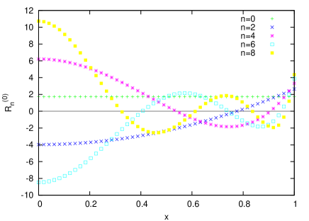
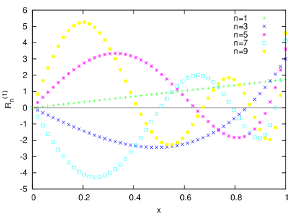
Figure 1: Radial part $R_{n}^{(l)}(x)$ of the 3D Zernike basis defined in (30), $l=0$ or $1$.

A.2 Fourier Transform

The Rayleigh expansion of the plane wave leads to the Fourier transform in terms of spherical Bessel Functions $j$ (Abramowitz and Stegun, 1972, sect. 10),

$$Z_{n,l}^{(m)}(\bm{\sigma})=\int d^{3}xe^{2\pi i\bm{\sigma}\cdot\bm{x}}R_{n}^{(l)}(x)Y_{l}^{m}(\theta,\phi)=4\pi i^{l}Y_{l}^{m}(\theta_{\sigma},\phi_{\sigma})\int_{0}^{1}x^{2}dxj_{l}(2\pi\sigma x)R_{n}^{(l)}(x).$$ (33)

Repeated use of the partial integration (Abramowitz and Stegun, 1972, 11.3.3)

$$\int x^{\mu+1}\mathcal{C}_{\nu-1}(x)dx=x^{\mu+1}\mathcal{C}_{\nu}(x)+(\nu-\mu-1)\int x^{\mu}\mathcal{C}_{\nu}(x)dx$$ (34)

for any ordinary Bessel Functions $\mathcal{C}$ yields

$$\int_{0}^{1}x^{2}dxj_{l}(2\pi\sigma x)x^{l+2s}=\frac{1}{2\pi\sigma}\sum_{k=0}^{s}(-1)^{k}\frac{s(s-1)(s-2)\cdots(s-k+1)}{(\pi\sigma)^{k}}j_{l+k+1}(2\pi\sigma)=\frac{1}{2\pi\sigma}\sum_{k=0}^{s}\frac{(-s)_{k}}{(\pi\sigma)^{k}}j_{l+k+1}(2\pi\sigma).$$ (35)

This is the building block to transform the radial polynomials of interest, ie, those constructable from non-negative integers $s$. Pochhammer’s symbol (Abramowitz and Stegun, 1972, 6.1.22)

$$(z)_{m}\equiv z(z+1)(z+2)\cdots(z+m-1)=\Gamma(z+m)/\Gamma(z);\quad(z)_{0}\equiv 1,$$ (36)

has been used to condense the notation for the falling factorials. Summation over $\alpha$ terms of this type yields

$$\int_{0}^{1}x^{2}j_{l}(2\pi\sigma x)x^{l}G_{\alpha}(q,q,x^{2})dx=\frac{1}{2\pi\sigma}\frac{\alpha!}{\Gamma(2\alpha+q)}\sum_{k=0}^{\alpha}\left(-\frac{1}{\pi\sigma}\right)^{k}j_{l+k+1}(2\pi\sigma)\Gamma(\alpha+q+k){\alpha\choose k}.$$ (37)

Gathering also the constant of normalization in (30) concludes

$$R_{n}^{(l)}(\sigma) \equiv \int_{0}^{1}x^{2}j_{l}(2\pi\sigma x)R_{n}^{(l)}(x)dx=\frac{\sqrt{2n+3}}{2\pi\sigma}\sum_{k=0}^{\alpha}\left(-\frac{1}{\pi\sigma}\right)^{k}j_{l+k+1}(2\pi\sigma)(\alpha+q)_{k}{\alpha\choose k}$$ (38)

$$= (-1)^{\alpha}\sqrt{2n+3}\,\frac{j_{n+1}(2\pi\sigma)}{2\pi\sigma},$$ (39)

orthogonal with

$$\int_{0}^{\infty}\sigma^{2}R_{n}^{(l)}(\sigma)R_{n^{\prime}}^{(l)}(\sigma)d\sigma=\frac{1}{(4\pi)^{2}}\delta_{nn^{\prime}}.$$ (40)

A graphical representation of the cases $l\leq 3$, $\alpha\leq 3$ is in Figure 2. The leading polynomial order is $R_{n}^{(l)}(\sigma)\propto\sigma^{n}$ as $\sigma\to 0$. (Abramowitz and Stegun, 1972, 10.1.2).

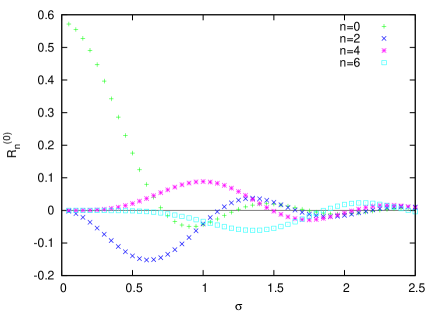
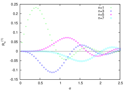
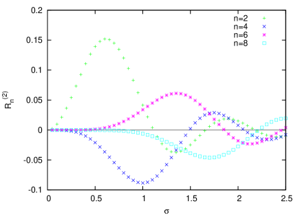
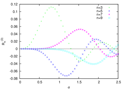
Figure 2: The simplest cases of $R_{n}^{(l)}(\sigma)$, $0\leq l\leq 3$, $\alpha\leq 3$, as given in (39).

In summary, (33) has been factorized as

$$Z_{n,l}^{(m)}(\bm{\sigma})=4\pi i^{l}Y_{l}^{m}(\theta_{\sigma},\phi_{\sigma})R_{n}^{(l)}(\sigma),$$ (41)

where Parseval’s theorem maintains orthogonality in wavenumber space,

$$\int d^{3}\sigma{Z_{n,l}^{(m)}}^{*}(\bm{\sigma})Z_{n^{\prime},l}^{(m^{\prime})}(\bm{\sigma})=\delta_{n,n^{\prime}}\delta_{m,m^{\prime}}.$$ (42)

Appendix B Mode List

The dominant modes $K_{p}^{(l)}$ of (16) are listed below, separated by empty lines, each representing $2l+1$ modes labeled by $m$. The notation consists of the value $\lambda_{p,l}^{2}$ followed by a colon, followed by $l$, followed by another colon and the Zernike expansion. The Zernike expansion is a sum over floating point numbers $\kappa_{n,l,p}$ multiplied by $Z_{n,l}^{(m)}$, the latter written as Z(n,l), optionally wrapped into a new line. The squares of $\kappa_{n,l,p}$ add to unity in each line. The phase/sign convention for the eigenvectors is that $\kappa_{n,l,p}$ with maximum absolute value is positive in each line.

Small-terms contributions with $|\kappa_{n,l,p}|<10^{-6}$ are not printed.

0.2723742 :  1:  +0.9935210*Z(1,1) -0.1132657*Z(3,1) +0.0093216*Z(5,1) -0.0001473*Z(7,1) +0.0000128*Z(9,1)
+0.0000014*Z(11,1)

0.0495069 :  2:  +0.9722349*Z(2,2) -0.2319940*Z(4,2) +0.0305878*Z(6,2) -0.0015909*Z(8,2) +0.0000930*Z(10,2)
+0.0000023*Z(12,2) +0.0000011*Z(14,2)

0.0495069 :  0:  +0.9722349*Z(2,0) -0.2319940*Z(4,0) +0.0305878*Z(6,0) -0.0015909*Z(8,0) +0.0000930*Z(10,0)
+0.0000023*Z(12,0) +0.0000011*Z(14,0)

0.0174576 :  3:  +0.9473332*Z(3,3) -0.3153328*Z(5,3) +0.0557030*Z(7,3) -0.0046947*Z(9,3) +0.0003314*Z(11,3)
-0.0000056*Z(13,3) +0.0000023*Z(15,3)

0.0143736 :  1:  +0.1081177*Z(1,1) +0.9173415*Z(3,1) -0.3757763*Z(5,1) +0.0743888*Z(7,1) -0.0072975*Z(9,1)
+0.0005484*Z(11,1) -0.0000162*Z(13,1) +0.0000031*Z(15,1)

0.0080675 :  4:  +0.9224733*Z(4,4) -0.3771734*Z(6,4) +0.0818302*Z(8,4) -0.0092993*Z(10,4) +0.0008094*Z(12,4)
-0.0000345*Z(14,4) +0.0000046*Z(16,4)

0.0059302 :  2:  +0.2144266*Z(2,2) +0.8327378*Z(4,2) -0.4927135*Z(6,2) +0.1320534*Z(8,2) -0.0189879*Z(10,2)
+0.0019187*Z(12,2) -0.0001183*Z(14,2) +0.0000100*Z(16,2)

0.0059302 :  0:  +0.2144266*Z(2,0) +0.8327378*Z(4,0) -0.4927135*Z(6,0) +0.1320534*Z(8,0) -0.0189879*Z(10,0)
+0.0019187*Z(12,0) -0.0001183*Z(14,0) +0.0000100*Z(16,0)

0.0043466 :  5:  +0.8987736*Z(5,5) -0.4247285*Z(7,5) +0.1076118*Z(9,5) -0.0151323*Z(11,5) +0.0015784*Z(13,5)
-0.0000988*Z(15,5) +0.0000094*Z(17,5)

0.0030561 :  3:  +0.2833231*Z(3,3) +0.7478488*Z(5,3) -0.5687499*Z(7,3) +0.1890304*Z(9,3) -0.0349457*Z(11,3)
+0.0044522*Z(13,3) -0.0003824*Z(15,3) +0.0000310*Z(17,3)

0.0028433 :  1:  +0.0312484*Z(1,1) +0.3323629*Z(3,1) +0.6982757*Z(5,1) -0.5956983*Z(7,1) +0.2106757*Z(9,1)
-0.0412113*Z(11,1) +0.0054932*Z(13,1) -0.0004989*Z(15,1) +0.0000407*Z(17,1)

0.0025891 :  6:  +0.8765467*Z(6,6) -0.4622201*Z(8,6) +0.1324035*Z(10,6) -0.0219219*Z(12,6) +0.0026626*Z(14,6)
-0.0002124*Z(16,6) +0.0000189*Z(18,6)

0.0017869 :  4:  +0.3306586*Z(4,4) +0.6685227*Z(6,4) -0.6180700*Z(8,4) +0.2423796*Z(10,4) -0.0539894*Z(12,4)
+0.0082606*Z(14,4) -0.0008873*Z(16,4) +0.0000803*Z(18,4) -0.0000033*Z(20,4) +0.0000010*Z(22,4)

0.0016562 :  7:  +0.8558181*Z(7,7) -0.4923231*Z(9,7) +0.1559183*Z(11,7) -0.0294312*Z(13,7) +0.0040659*Z(15,7)
-0.0003881*Z(17,7) +0.0000358*Z(19,7)

0.0015654 :  2:  -0.0803297*Z(2,2) -0.4131467*Z(4,2) -0.5450977*Z(6,2) +0.6585434*Z(8,2) -0.2941911*Z(10,2)
+0.0731123*Z(12,2) -0.0122479*Z(14,2) +0.0014490*Z(16,2) -0.0001385*Z(18,2) +0.0000078*Z(20,2)
-0.0000014*Z(22,2)

0.0015654 :  0:  -0.0803297*Z(2,0) -0.4131467*Z(4,0) -0.5450977*Z(6,0) +0.6585434*Z(8,0) -0.2941911*Z(10,0)
+0.0731123*Z(12,0) -0.0122479*Z(14,0) +0.0014490*Z(16,0) -0.0001385*Z(18,0) +0.0000078*Z(20,0)
-0.0000014*Z(22,0)

0.0011353 :  5:  -0.3644454*Z(5,5) -0.5960909*Z(7,5) +0.6491312*Z(9,5) -0.2909694*Z(11,5) +0.0750988*Z(13,5)
-0.0133381*Z(15,5) +0.0016997*Z(17,5) -0.0001754*Z(19,5) +0.0000115*Z(21,5) -0.0000017*Z(23,5)

0.0011176 :  8:  +0.8365082*Z(8,8) -0.5168302*Z(10,8) +0.1780536*Z(12,8) -0.0374644*Z(14,8)
+0.0057793*Z(16,8) -0.0006360*Z(18,8) +0.0000629*Z(20,8) -0.0000023*Z(22,8) +0.0000010*Z(24,8)

0.0009624 :  3:  -0.1234664*Z(3,3) -0.4534598*Z(5,3) -0.4075425*Z(7,3) +0.6822917*Z(9,3) -0.3674242*Z(11,3)
+0.1096522*Z(13,3) -0.0219805*Z(15,3) +0.0031596*Z(17,3) -0.0003567*Z(19,3) +0.0000288*Z(21,3)
-0.0000031*Z(23,3)

0.0009269 :  1:  -0.0132054*Z(1,1) -0.1534280*Z(3,1) -0.4633881*Z(5,1) -0.3595625*Z(7,1) +0.6845747*Z(9,1)
-0.3857727*Z(11,1) +0.1191289*Z(13,1) -0.0245691*Z(15,1) +0.0036299*Z(17,1) -0.0004190*Z(19,1)
+0.0000351*Z(21,1) -0.0000037*Z(23,1)

0.0007862 :  9:  +0.8185038*Z(9,9) -0.5369951*Z(11,9) +0.1988032*Z(13,9) -0.0458634*Z(15,9)
+0.0077854*Z(17,9) -0.0009640*Z(19,9) +0.0001032*Z(21,9) -0.0000060*Z(23,9) +0.0000014*Z(25,9)

0.0007655 :  6:  -0.3891945*Z(6,6) -0.5304668*Z(8,6) +0.6673369*Z(10,6) -0.3345193*Z(12,6) +0.0974584*Z(14,6)
-0.0196069*Z(16,6) +0.0028703*Z(18,6) -0.0003351*Z(20,6) +0.0000280*Z(22,6) -0.0000032*Z(24,6)

0.0006365 :  4:  -0.1595289*Z(4,4) -0.4702764*Z(6,4) -0.2875787*Z(8,4) +0.6806273*Z(10,4) -0.4291202*Z(12,4)
+0.1485535*Z(14,4) -0.0344854*Z(16,4) +0.0057898*Z(18,4) -0.0007570*Z(20,4) +0.0000753*Z(22,4)
-0.0000076*Z(24,4)

0.0005909 :  2:  -0.0387797*Z(2,2) -0.2229036*Z(4,2) -0.4693503*Z(6,2) -0.1796996*Z(8,2) +0.6673417*Z(10,2)
-0.4675801*Z(12,2) +0.1742073*Z(14,2) -0.0429519*Z(16,2) +0.0076259*Z(18,2) -0.0010468*Z(20,2)
+0.0001105*Z(22,2) -0.0000110*Z(24,2)

0.0005909 :  0:  -0.0387797*Z(2,0) -0.2229036*Z(4,0) -0.4693503*Z(6,0) -0.1796996*Z(8,0) +0.6673417*Z(10,0)
-0.4675801*Z(12,0) +0.1742073*Z(14,0) -0.0429519*Z(16,0) +0.0076259*Z(18,0) -0.0010468*Z(20,0)
+0.0001105*Z(22,0) -0.0000110*Z(24,0)

0.0005719 : 10:  +0.8016857*Z(10,10) -0.5537242*Z(12,10) +0.2182106*Z(14,10) -0.0545025*Z(16,10)
+0.0100622*Z(18,10) -0.0013779*Z(20,10) +0.0001598*Z(22,10) -0.0000118*Z(24,10) +0.0000020*Z(26,10)

0.0005398 :  7:  -0.4076451*Z(7,7) -0.4711126*Z(9,7) +0.6763013*Z(11,7) -0.3731525*Z(13,7) +0.1204400*Z(15,7)
-0.0269500*Z(17,7) +0.0044332*Z(19,7) -0.0005783*Z(21,7) +0.0000570*Z(23,7) -0.0000061*Z(25,7)

0.0004436 :  5:  -0.1893914*Z(5,5) -0.4728633*Z(7,5) -0.1841723*Z(9,5) +0.6623861*Z(11,5) -0.4795241*Z(13,5)
+0.1880973*Z(15,5) -0.0494097*Z(17,5) +0.0094393*Z(19,5) -0.0014015*Z(21,5) +0.0001624*Z(23,5)
-0.0000171*Z(25,5)

0.0004276 : 11:  +0.7859404*Z(11,11) -0.5676904*Z(13,11) +0.2363442*Z(15,11) -0.0632823*Z(17,11)
+0.0125856*Z(19,11) -0.0018812*Z(21,11) +0.0002354*Z(23,11) -0.0000206*Z(25,11) +0.0000029*Z(27,11)

0.0004024 :  3:  -0.0651981*Z(3,3) -0.2733637*Z(5,3) -0.4451931*Z(7,3) -0.0326736*Z(9,3) +0.6203023*Z(11,3)
-0.5285997*Z(13,3) +0.2303104*Z(15,3) -0.0658223*Z(17,3) +0.0135712*Z(19,3) -0.0021567*Z(21,3)
+0.0002690*Z(23,3) -0.0000292*Z(25,3) +0.0000019*Z(27,3)

0.0003943 :  8:  -0.4215561*Z(8,8) -0.4173790*Z(10,8) +0.6785254*Z(12,8) -0.4071763*Z(14,8)
+0.1435708*Z(16,8) -0.0352331*Z(18,8) +0.0064074*Z(20,8) -0.0009229*Z(22,8) +0.0001035*Z(24,8)
-0.0000112*Z(26,8)

0.0003932 :  1:  -0.0068258*Z(1,1) -0.0831481*Z(3,1) -0.2897187*Z(5,1) -0.4325853*Z(7,1) +0.0025750*Z(9,1)
+0.6065149*Z(11,1) -0.5392619*Z(13,1) +0.2411059*Z(15,1) -0.0703318*Z(17,1) +0.0147685*Z(19,1)
-0.0023858*Z(21,1) +0.0003027*Z(23,1) -0.0000331*Z(25,1) +0.0000022*Z(27,1)

0.0003271 : 12:  +0.7711645*Z(12,12) -0.5794048*Z(14,12) +0.2532829*Z(16,12) -0.0721245*Z(18,12)
+0.0153311*Z(20,12) -0.0024758*Z(22,12) +0.0003325*Z(24,12) -0.0000329*Z(26,12) +0.0000043*Z(28,12)

0.0003217 :  6:  -0.2141615*Z(6,6) -0.4666186*Z(8,6) -0.0954608*Z(10,6) +0.6334239*Z(12,6) -0.5195267*Z(14,6)
+0.2270429*Z(16,6) -0.0663391*Z(18,6) +0.0141531*Z(20,6) -0.0023475*Z(22,6) +0.0003081*Z(24,6)
-0.0000351*Z(26,6) +0.0000025*Z(28,6)

0.0002963 :  9:  -0.4321073*Z(9,9) -0.3686297*Z(11,9) +0.6757850*Z(13,9) -0.4369714*Z(15,9)
+0.1665011*Z(17,9) -0.0443179*Z(19,9) +0.0087990*Z(21,9) -0.0013848*Z(23,9) +0.0001726*Z(25,9)
-0.0000196*Z(27,9) +0.0000011*Z(29,9)

0.0002873 :  4:  +0.0899412*Z(4,4) +0.3087998*Z(6,4) +0.4055501*Z(8,4) -0.0847063*Z(10,4) -0.5563662*Z(12,4)
+0.5704152*Z(14,4) -0.2846000*Z(16,4) +0.0922604*Z(18,4) -0.0215806*Z(20,4) +0.0038876*Z(22,4)
-0.0005548*Z(24,4) +0.0000668*Z(26,4) -0.0000059*Z(28,4)

0.0002739 :  2:  +0.0217345*Z(2,2) +0.1326368*Z(4,2) +0.3344713*Z(6,2) +0.3619721*Z(8,2) -0.1549178*Z(10,2)
-0.5119804*Z(12,2) +0.5869219*Z(14,2) -0.3108572*Z(16,2) +0.1054741*Z(18,2) -0.0256715*Z(20,2)
+0.0047925*Z(22,2) -0.0007084*Z(24,2) +0.0000877*Z(26,2) -0.0000082*Z(28,2) +0.0000011*Z(30,2)

0.0002739 :  0:  +0.0217345*Z(2,0) +0.1326368*Z(4,0) +0.3344713*Z(6,0) +0.3619721*Z(8,0) -0.1549178*Z(10,0)
-0.5119804*Z(12,0) +0.5869219*Z(14,0) -0.3108572*Z(16,0) +0.1054741*Z(18,0) -0.0256715*Z(20,0)
+0.0047925*Z(22,0) -0.0007084*Z(24,0) +0.0000877*Z(26,0) -0.0000082*Z(28,0) +0.0000011*Z(30,0)

0.0002552 : 13:  +0.7572651*Z(13,13) -0.5892625*Z(15,13) +0.2691084*Z(17,13) -0.0809680*Z(19,13)
+0.0182744*Z(21,13) -0.0031620*Z(23,13) +0.0004537*Z(25,13) -0.0000497*Z(27,13) +0.0000062*Z(29,13)

0.0002407 :  7:  -0.2348116*Z(7,7) -0.4548404*Z(9,7) -0.0194882*Z(11,7) +0.5976955*Z(13,7) -0.5502531*Z(15,7)
+0.2645281*Z(17,7) -0.0848500*Z(19,7) +0.0199308*Z(21,7) -0.0036443*Z(23,7) +0.0005316*Z(25,7)
-0.0000659*Z(27,7) +0.0000060*Z(29,7)

0.0002280 : 10:  -0.4401180*Z(10,10) -0.3242846*Z(12,10) +0.6693673*Z(14,10) -0.4629349*Z(16,10)
+0.1889767*Z(18,10) -0.0540704*Z(20,10) +0.0116042*Z(22,10) -0.0019775*Z(24,10) +0.0002699*Z(26,10)
-0.0000326*Z(28,10) +0.0000025*Z(30,10)

0.0002127 :  5:  +0.1122926*Z(5,5) +0.3328253*Z(7,5) +0.3585602*Z(9,5) -0.1767793*Z(11,5) -0.4838664*Z(13,5)
+0.5954557*Z(15,5) -0.3351895*Z(17,5) +0.1212944*Z(19,5) -0.0316439*Z(21,5) +0.0063570*Z(23,5)
-0.0010169*Z(25,5) +0.0001357*Z(27,5) -0.0000143*Z(29,5) +0.0000018*Z(31,5)

0.0002025 : 14:  +0.7441600*Z(14,14) -0.5975741*Z(16,14) +0.2839011*Z(18,14) -0.0897649*Z(20,14)
+0.0213924*Z(22,14) -0.0039392*Z(24,14) +0.0006007*Z(26,14) -0.0000717*Z(28,14) +0.0000090*Z(30,14)

0.0001994 :  3:  +0.0387722*Z(3,3) +0.1746705*Z(5,3) +0.3544766*Z(7,3) +0.2795820*Z(9,3) -0.2630382*Z(11,3)
-0.4046044*Z(13,3) +0.6071129*Z(15,3) -0.3742479*Z(17,3) +0.1447577*Z(19,3) -0.0399704*Z(21,3)
+0.0084474*Z(23,3) -0.0014183*Z(25,3) +0.0001974*Z(27,3) -0.0000221*Z(29,3) +0.0000026*Z(31,3)

0.0001963 :  1:  +0.0039977*Z(1,1) +0.0501564*Z(3,1) +0.1886747*Z(5,1) +0.3560673*Z(7,1) +0.2581983*Z(9,1)
-0.2814148*Z(11,1) -0.3836754*Z(13,1) +0.6083843*Z(15,1) -0.3837324*Z(17,1) +0.1508905*Z(19,1)
-0.0422465*Z(21,1) +0.0090396*Z(23,1) -0.0015357*Z(25,1) +0.0002159*Z(27,1) -0.0000245*Z(29,1)
+0.0000029*Z(31,1)

0.0001848 :  8:  +0.2521278*Z(8,8) +0.4396161*Z(10,8) -0.0455476*Z(12,8) -0.5579080*Z(14,8)
+0.5728641*Z(16,8) -0.2999791*Z(18,8) +0.1045395*Z(20,8) -0.0267374*Z(22,8) +0.0053315*Z(24,8)
-0.0008530*Z(26,8) +0.0001150*Z(28,8) -0.0000121*Z(30,8) +0.0000016*Z(32,8)

0.0001789 : 11:  -0.4461735*Z(11,11) -0.2838305*Z(13,11) +0.6602212*Z(15,11) -0.4854523*Z(17,11)
+0.2108168*Z(19,11) -0.0643653*Z(21,11) +0.0148112*Z(23,11) -0.0027123*Z(25,11) +0.0004011*Z(27,11)
-0.0000515*Z(29,11) +0.0000047*Z(31,11)

0.0001630 : 15:  +0.7317763*Z(15,15) -0.6045873*Z(17,15) +0.2977377*Z(19,15) -0.0984783*Z(21,15)
+0.0246634*Z(23,15) -0.0048055*Z(25,15) +0.0007755*Z(27,15) -0.0000998*Z(29,15) +0.0000127*Z(31,15)

0.0001621 :  6:  +0.1321892*Z(6,6) +0.3482620*Z(8,6) +0.3088642*Z(10,6) -0.2477773*Z(12,6) -0.4081762*Z(14,6)
+0.6063296*Z(16,6) -0.3809198*Z(18,6) +0.1519987*Z(20,6) -0.0436556*Z(22,6) +0.0096556*Z(24,6)
-0.0017060*Z(26,6) +0.0002504*Z(28,6) -0.0000300*Z(30,6) +0.0000036*Z(32,6)

0.0001501 :  4:  +0.0559858*Z(4,4) +0.2088990*Z(6,4) +0.3571657*Z(8,4) +0.1959894*Z(10,4) -0.3351164*Z(12,4)
-0.2950686*Z(14,4) +0.6047083*Z(16,4) -0.4289290*Z(18,4) +0.1863726*Z(20,4) -0.0574666*Z(22,4)
+0.0135356*Z(24,4) -0.0025371*Z(26,4) +0.0003927*Z(28,4) -0.0000500*Z(30,4) +0.0000060*Z(32,4)

References

- Abramowitz and Stegun (1972) Abramowitz, M., and I. A. Stegun (eds.), 1972, Handbook of Mathematical Functions (Dover Publications, New York), 9th edition, ISBN 0-486-61272-4.
- Altmann (1957) Altmann, S. L., 1957, Proc. Cambr. Phil. Soc. 53(2), 343.
- Bhatia and Wolf (1952) Bhatia, A. B., and E. Wolf, 1952, Proc. Phys. Soc. B 65(11), 909.
- Bhatia and Wolf (1954) Bhatia, A. B., and E. Wolf, 1954, Proc. Cambr. Phil. Soc. 50(1), 40.
- Bradley and Cracknell (1972) Bradley, C. J., and A. P. Cracknell, 1972, The Mathematical Theory of the Symmetry in Solids (Clarendon Press, Oxford).
- Conan (2000) Conan, R., 2000, Modélisation des effets de l’échelle externe de cohérence spatiale du front d’onde pour l’observation à Haute Résolution Angulaire en Astronomie, Ph.D. thesis, Université de Nice.
- Conan (2008) Conan, R., 2008, J. Opt. Soc. Am. A 25(2), 526.
- Dai (1995) Dai, G.-m., 1995, J. Opt. Soc. Am. A 12(10), 2182.
- Edmonds (1957) Edmonds, A. R., 1957, Angular momentum in quantum mechanics (Princeton University Press).
- Fried (1965) Fried, D. L., 1965, J. Opt. Soc. Am. 55(11), 1427, E: Fried (1966b).
- Fried (1966a) Fried, D. L., 1966a, J. Opt. Soc. Am. 56(10), 1372.
- Fried (1966b) Fried, D. L., 1966b, J. Opt. Soc. Am. 56(3), 410E.
- Fried (1978) Fried, D. L., 1978, J. Opt. Soc. Am. 68(12), 1651.
- Gradstein and Ryshik (1981) Gradstein, I., and I. Ryshik, 1981, Summen-, Produkt- und Integraltafeln (Harri Deutsch, Thun), 1st edition, ISBN 3-87144-350-6.
- Hufnagel and Stanley (1964) Hufnagel, R. E., and N. R. Stanley, 1964, J. Opt. Soc. Am. 54(1), 52.
- Magnus and Oberhettinger (1948) Magnus, W., and F. Oberhettinger, 1948, Formeln und Sätze für die speziellen Funktionen der Mathematischen Physik, volume 52 of Die Grundlehren der mathematischen Wissenschaften in Einzeldarstellungen (Springer, Berlin, Heidelberg), 2nd edition.
- Mak et al. (2008) Mak, L., S. Grandison, and R. J. Morris, 2008, J. Mol. Graph. Model. 26(7), 1035.
- Mathar (2002) Mathar, R. J., 2002, Int. J. Quant. Chem. 90(1), 227.
- Mathar (2007a) Mathar, R. J., 2007a, arXiv:astro-ph/0705.1700 .
- Mathar (2007b) Mathar, R. J., 2007b, arXiv:math.NA/0705.1329 .
- Noll (1976) Noll, R. J., 1976, J. Opt. Soc. Am. 66(3), 207.
- Novotni and Klein (2003) Novotni, M., and R. Klein, 2003, in Proc. Eigth ACM Symposium on Solid Modeling and Applications (Association for Computing Machinery, Seattle, Washington, USA), ACM Symposium on Solid and Physical Modeling, pp. 216–225.
- Novotni and Klein (2004) Novotni, M., and R. Klein, 2004, Computer-Aided Design 36(11), 1047.
- Pérez and Zunino (2008) Pérez, D. G., and L. Zunino, 2008, Opt. Lett. 33(6), 572.
- Roddier (1981) Roddier, F., 1981 (North Holland, Amsterdam), volume 19 of Prog. Opt., pp. 281–376.
- Roddier (1990) Roddier, N., 1990, Opt. Eng. 29(10), 1174.
- Strohbein (1971) Strohbein, J. W., 1971 (North-Holland, Amsterdam), volume 9 of Prog. Opt., pp. 73–122.