Alignment of the Pixel and SCT Modules for the 2004 ATLAS Combined Test Beam

Abstract

A small set of final prototypes of the ATLAS Inner Detector silicon tracker (Pixel and SCT) were used to take data during the 2004 Combined Test Beam. Data were collected from runs with beams of different flavour (electrons, pions, muons and photons) with a momentum range of 2 to 180 GeV/c. Four independent methods were used to align the silicon modules. The corrections obtained were validated using the known momenta of the beam particles and were shown to yield consistent results among the different alignment approaches. From the residual distributions, it is concluded that the precision attained in the alignment of the silicon modules is of the order of 5 $\mu$m in their most precise coordinate.

1 Introduction

This note reports the results of the alignment of the ATLAS Inner Detector [1] silicon tracker (Pixel and SCT) modules at the ATLAS Combined Test Beam data-taking (CTB) which took place at the CERN H8 beam-test facility in 2004. The purpose of the CTB was to study the combined performance of ATLAS. The setup represented a full barrel slice of the Inner Detector (ID), Calorimeter and Muon Spectrometer of the complete ATLAS detector and was instrumented with final prototypes.

Once the Pixel and SCT modules had been installed in the CTB setup in addition to the already operational TRT, the Inner Detector was fully integrated into the common data acquisition system. Data were collected with this fully integrated ID, using beams with different characteristics. Pion, electron, muon and photon beams were used in a wide range of momenta from 2 to 180 $GeV/c$, and some data were taken without magnetic field (B).

The CTB setup represented an ideal framework for testing the Inner Detector software. The offline reconstruction was tested on real data using the ATLAS software framework (ATHENA) [2] and was particularly useful for tracking [3], pre-commissioning tests, and for testing the alignment software.

Determining the locations of the tracking detector elements is crucial for the performance of the ID tracker. For this purpose, various alignment algorithms, based on optimization of track hit residuals, were applied to align the CTB silicon setup. An alignment algorithm specifically developed for the CTB (hereafter referred to as Valencia approach [4]) had been adapted from an algorithm used in previous SCT standalone test beams [5], by the time the first data were collected. The Valencia approach produced alignment corrections for the initial CTB data analysis. For the final analysis of the alignment, three more algorithms were tested. These algorithms, developed for the alignment of the entire Inner Detector silicon tracker, are: Robust [6], Local $\chi^{2}$ [7, 8] and Global $\chi^{2}$ [9, 10] approaches [11].

The resulting sets of alignment constants were used to measure the momenta of the incident particles in electron and pion runs. A comparison with the nominal momenta was used to crosscheck the different alignment procedures. The residual distributions and reconstructed track parameters were studied for electrons and pions with and without B field. The global reference frame was also studied by matching the alignment results via a global offset optimization.

2 Setup, Data Samples and Tracking

The Inner Detector volume in the CTB setup was divided into three containers for each sub-detector: Pixel, SCT and TRT. Six Pixel and eight SCT modules were placed in their respective containers. The TRT setup consisted of two barrel wedges, equivalent to 1/16 of the circumference of a cylinder.

The coordinate system was chosen to be right-handed, with the $X$-axis along the beam direction and the $Y$-axis pointing vertically upward as depicted in Fig. 1 [12]. The origin was located at the entrance of the dipole magnet that produced a maximum 1.4 T field in the negative Z-direction. The Pixel and SCT detectors were located inside the magnet whereas the TRT detector was located outside due to its larger dimension.

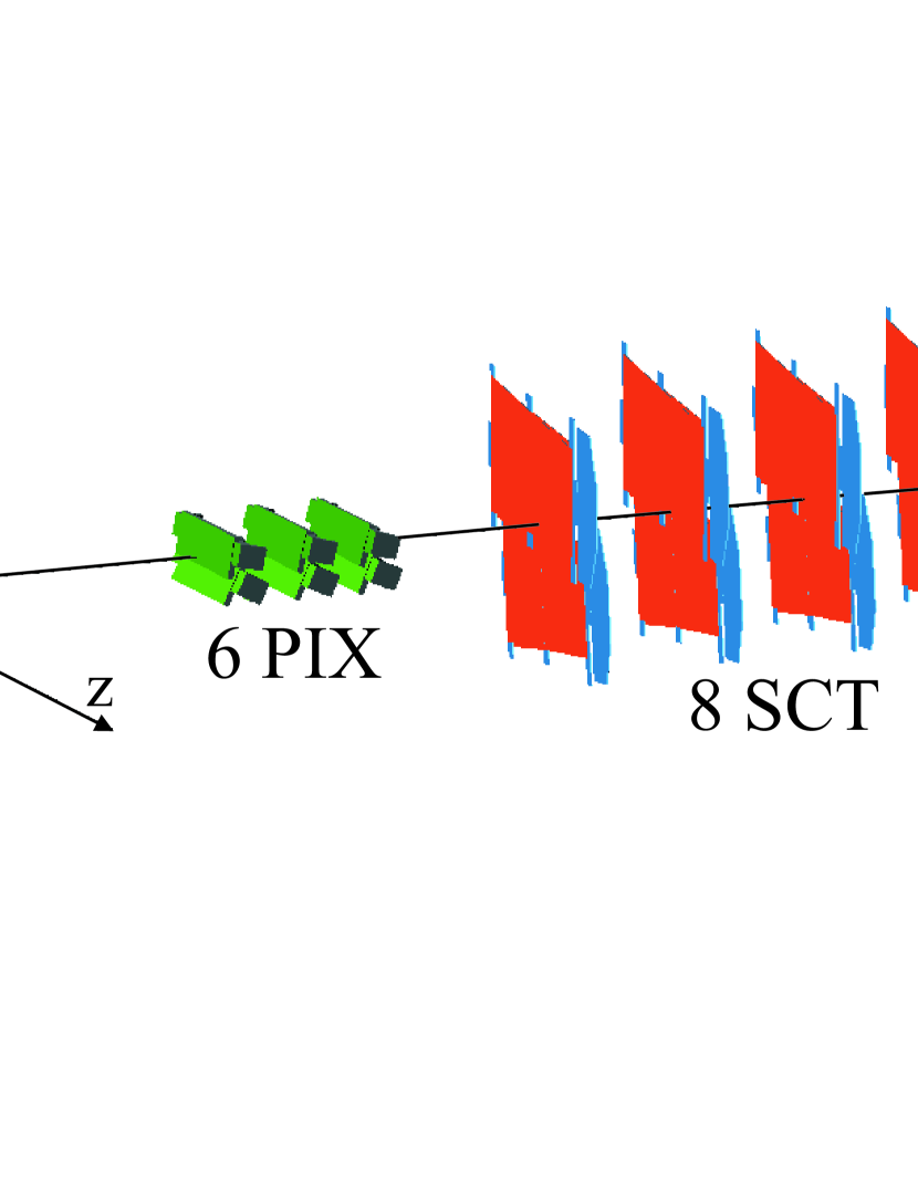
Figure 1: Schematic representation of the ID components and the magnet at the CTB. The reference coordinate system is also shown. The long pixel coordinate and the SCT module strips are almost parallel to the $Z$-axis.

A Pixel module [13, 14] consists of a single silicon wafer with an array of 50$\times$400 $\mu$m² pixels that are read out by 16 chips [15]. The active area of each module is $\sim 60.8\times 16.4{\mathrm{\ mm}}^{2}$. In the CTB setup, six Pixel modules were distributed in three layers (0,1,2) and two sectors (0,1). The distances along the beam axis between the different layers and the locations of modules within each layer mimic the arrangement of the modules in ATLAS. The first Pixel layer was nominally located at 195.986 mm from the global coordinate center along the beamline ($X$-axis) and the last layer was located at 268.277 mm. Each module was positioned at an angle of about $20^{\circ}$ with respect to the incident beam, around the long pixel coordinate. Modules in the same layer overlapped by $\sim 200~{}\mu$m.

A SCT module is built from four single-sided silicon microstrip sensors glued back to back in pairs with 40 mrad stereo angle for a 3D space-point reconstruction [16, 17]. The modules produce two hits, one in each plane. The SCT end-cap modules have a wedge-shaped geometry which results in variable pitch sizes (Fig. 5). In the CTB setup, one of the four shape-wise distinct SCT end-cap module types was used (outer module). For the outer end-cap modules, the readout strip pitch is 70.9-81.1 $\mu$m. Each plane has a length of about 120.0 ${\mathrm{\ mm}}$ and bases of about $72.0~{}{\mathrm{\ mm}}$ and $57.0~{}{\mathrm{\ mm}}$. The readout is provided by a binary chip [18]. Eight SCT modules were used in each of the four layers (0,3) of the CTB setup; distributed in two sectors (0,1) with a $4{\mathrm{\ mm}}$ overlap. The arrangement of the modules was similar to the SCT barrel configuration in ATLAS, however, the modules were not mounted at an angle with respect to the beam axis. The SCT modules were nominally positioned from 378.198 mm to 598.218 mm along the beam axis.

The beam-line instrumentation, including trigger and veto scintillators, Cherenkov counters and readout system is documented elsewhere [19, 20]. The Inner Detector magnetic field profile was measured[12] and its non-uniformity was taken into account during the track reconstruction. The absolute momentum as measured by the silicon detector which was located in a very uniform magnetic field region was certified to better than 1$\%$ by comparing the momentum reconstructed from silicon alone with that obtained independently using the angular measurement in the TRT.

The CTB ID data taking was divided into five different periods between September 2004 and November 2004 [12], where 22 million usable events were collected. In order to evaluate the material effects in the tracker, aluminum plates (10% $X_{0}$) were inserted and removed between the Pixel, SCT and TRT setups (Fig. 1) in alternate runs. The TRT was repositioned in the transverse plane of the beam. Particle type and energy of the beam also alternated during the periods.

The algorithms provided a valid silicon detector alignment for all the CTB data-taking periods. However, this article reports on the last period (period 5) of stable data-taking when no extra material layers were used. Table 1 lists the runs used for alignment studies in this period. Events from run 2102355, a 100 GeV pion beam run without a B-field, were used as input to all algorithms for the production of alignment corrections. For the Local $\chi^{2}$ approach, two other pion runs were used in addition. Further event selection details are given in Section 3.

Table 1: List of selected runs used to assess the alignment results.

Run Number	Particle Type	Energy (GeV)	B field
2102355	$\pi$	100	Off
2102439	$e$	20	On
2102400	$e$	50	On
2102452	$e$	80	On
2102399	$e$	100	On
2102463	$e$	180	On
2102442	$\pi$	20	On
2102365	$\pi$	100	On

2.1 Simulation

The CTB setup was simulated with Geant 4 using the same geometry description as the event reconstruction. Detector positions and initial numbers were provided through an Oracle-based conditions database (look-up information) which allowed the five different periods to be distinguished from one another.

CTB specific modifications were applied to the simulation for studying the Pixel and SCT alignment, i.e. the propagation through material upstream of the ID and the inclusion of measured beam profiles. The upstream material (mainly air and triggering/monitoring scintillators) corresponded to 13.2% radiation lengths and was taken into account to mimic the momentum distribution in the data properly. Profiles, consisting of beam incidence positions and angles, were taken from the data and were applied during the upstream simulation to bring the simulated hit maps and residual distributions of the silicon modules into agreement with the data.

The magnetic field map was calculated taking into account the magnet geometry, in one quadrant of the transverse plane with respect to the beam axis. The remaining field map was modeled assuming a symmetric the field map around the main axis of the magnet. The field map calculated along these lines compares well with the actual measurement of the dipole field which were performed before and after the CTB runs.

2.2 Tracking and Reconstruction

The default tracking algorithm in the CTB was the ‘CTBTracking’ algorithm [3]. CTBTracking consists of a pattern recognition part, developed specially for the CTB, and a track fitting algorithm that is in use in full ATLAS as well as in the CTB. The pattern recognition finds the tracks by looping through combinations of space points. The track fitting algorithm is based on a global $\chi^{2}$ minimization technique, often called the ‘breakpoint’ method in the literature[21]. Multiple scattering and energy loss enter into the algorithm as additional fit parameters at a given number of scattering planes. The track fit has a custom description of the detector material in the test beam setup, with one scattering plane for each layer of silicon modules. This material description was precisely tuned to give the best possible track resolutions, down to very low energies (1 GeV or less). A number of options and features exist in the track fit that are particularly useful for the alignment algorithms, such as the possibility of setting the momentum to a fixed value in the fit, and the ability to retrieve the fitted scattering angles and their covariances.

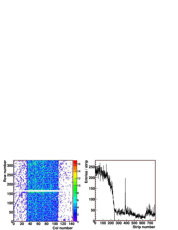
Figure 2: Left: Pixel hit map for 100 GeV pion runs. The $x$-axis corresponds to Pixel $\eta$-coordinate and the $y$-axis to Pixel $\phi$-coordinate. Empty horizontal bands correspond to the ganged pixels. Lighter vertical bands are due to the 600-$\mu$m-wide pixels. Right: SCT hit map for the same run.

Fig. 2 shows typical hit maps for a Pixel and SCT module. The illumination was rather uniform for the channels that lay within the scintillator trigger acceptance window in the central region ($\sim 3\times 3~{}\mbox{cm}^{2}$ wide). More details on the tracking performance of the pixel detectors can be found elsewhere [22]. Unmasked noisy channels can be distinguished in the SCT hitmap. Those that were masked during data-acquisition appear as zero-entry channels. The illumination was not uniform and limited along the strip length but only in the central region, where the sensor planes overlapped completely with the trigger scintillator.

The limited illumination of the sensors had direct consequences on some of the alignment degrees of freedom (DoF) due to insufficient constraints and reduced sensitivity. The problem was more severe for SCT modules, because the SCT modules were not tilted with respect to the beamline. As the beam incidence was almost perpendicular to the module planes, the alignment procedures were not very sensitive towards misalignments along the beam axis.

The pixel sensors require free space in order to bond the readout chips on the surface of the sensor. In the precise $\phi$ coordinate, unbonded pixels are physically connected to nearby pixels (ganged pixels) and share a readout logic channel. Due to this connection, whenever a hit was registered by a logic channel, there was an ambiguity as to which pixel fired. In the long coordinate wider pixels (600-$\mu$m instead of 400-$\mu$m) are used. The wider pixels collect more hits. The impact of both effects is clearly seen in the pixel module hit map (Fig. 2). The ambiguity in the ganged pixels was also found to effect the alignment. In a highly misaligned environment, tracking may make too many wrong decisions between ganged pixels. It was found that, in the presence of a high track quality cut, the ganged pixel hits were favoured, degrading the quality of the alignment [6].

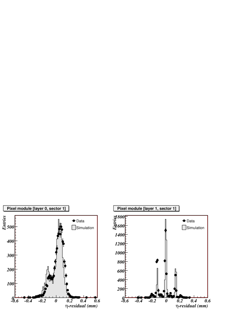
Figure 3: Pixel $\eta$-residuals for tracks reconstructed with Pixels and SCT. Left: first Pixel layer. Right: middle Pixel layer.

The fact that the modules were exposed to almost perpendicular beams resulted in discrete Pixel $\eta$-residual distributions. Due to the large dimension in this direction (400 $\mu m$ compared to 300 $\mu m$ of the thickness of the silicon bulk) the drift of the charge carriers along that direction is negligible. Therefore, almost all of the clusters consist of a single pixel in the $\eta$-coordinate. As the cluster position is located in its geometrical center, the outcome is a discrete positioning of clusters (Fig. 3). With only three pixel layers providing three precision points, a discrete residual distribution was obtained. The use of SCT clusters in the tracking partially removed this undesired effect [4]. Effectively the pixel $\eta$-residuals of the first and last pixel layers were somewhat broadened by overlaps of Gaussian distributions, while the middle layer $\eta$-residuals remained discrete. This peculiarity of the CTB setup made the alignment along the pixel $\eta$-coordinate difficult. ATLAS collision data will not present such difficulties.

3 Alignment of the CTB Data

The goal of alignment is to determine the corrections to the parameters that describe the position and orientation of the module in space. Each module is treated as a flat rigid body with 6 DoFs, i.e., three translations along the local coordinate axes ($x$, $y$, $z$) and three rotations ($\alpha$, $\beta$, $\gamma$) around the local coordinate axes, in a right-handed orthogonal frame where the origin is at the center-of-gravity of each module and the local $x$-coordinate is along the most precise coordinate. The translations correspond to the shift of the module with respect to its nominal position. For the axes orientation, the Cardano representation of angular rotation with respect to the cartesian axes was used. The alignment corrections were stored in the conditions database.

The alignment corrections are given in terms of CLHEP [23] transform objects $H$, made of a rotation matrix $R$ and a translation vector $\vec{T}$. The rotation matrix is defined as:

$$R=R_{x}(\alpha)\cdot R_{y}(\beta)\cdot R_{z}(\gamma)$$ (1)

with $\alpha$, $\beta$ and $\gamma$ being the rotation angles around the $x$, $y$ and $z$-axes. $R_{z}(\gamma)$ is the first rotation applied and $R_{x}(\alpha)$ the last. The representation of a point in the local reference frame ($\vec{P}$) of a module is $H\cdot\vec{P}=\vec{T}+R\cdot\vec{P}$ in the global frame. Lets consider $H_{0}$ as the transformation specifying the nominal position of a given module. If $\delta H$ is a shift of the module, the new transformation of the points measured by it becomes $H=H_{0}\cdot\delta H$. Therefore, the task of the alignment is to determine the 6 DoFs that define $\delta H$ for each module. In the case of poorly constrained movements, some DoFs may not be considered.

The technique to align each silicon module consists of minimizing its two residuals (pixel modules measure two coordinates and each SCT module has two sensor planes). The $i$-$th$ residual (defined by coordinate, plane or module) is thus $r_{i}\equiv(\vec{m_{i}}-\vec{e_{i}}(\mathbf{a},\mbox{\boldmath$\pi$}))\cdot\hat{k_{i}}$, where $\vec{m_{i}}$ represents the position of the hit recorded in the sensor plane, $\vec{e_{i}}$ is the intersection point of the extrapolated track to the detector that depends on the alignment parameters $(\mathbf{a})$ and the vector of track parameters $\mbox{\boldmath$\pi$}=(d_{0},\phi_{0},z_{0},\theta_{0},q/p)$. $\hat{k_{i}}$ denotes the unit vector of the measurement direction [9].

All alignment algorithms were run iteratively. Initially, nominal detector and hit positions were used for track reconstruction. After the track fit, residuals and their derivatives with respect to alignment and/or track parameters were calculated to determine the alignment corrections. For each module, the best fit estimates for alignment parameters were derived and its position was updated. A new reconstruction with updated module positions was performed and the alignment was reiterated. This procedure is expected to converge to final alignment corrections for each module and the residual resolution is expected to improve.

The alignment was performed using two different classes of approach. The Robust approach is based on iterative minimization of the residual means of overlapping and non-overlapping modules. The approach is “robust" because the output is stable against changes in the input tracking information.

The Valencia , Local $\chi^{2}$ and Global $\chi^{2}$ approaches are based on the linear least squares minimization defined for a set of reconstructed tracks as:

$$\chi^{2}(\mathbf{a},\mbox{\boldmath$\pi$}_{1},\dots,\mbox{\boldmath$\pi$}_{t})=\sum_{i\ \in\ tracks}{\mathbf{r}_{i}\,^{T}V_{i}^{-1}\mathbf{r}_{i}}$$ (2)

where $\mathbf{r}_{i}=\mathbf{r}_{i}(\mathbf{a},\mbox{\boldmath$\pi$}_{i})$ is the vector of residuals measured for the fitted track $i$. $V_{i}$ is the covariance matrix of the residual measurements of track $i$. The generic solution for alignment corrections ($\delta\mathbf{a}$) is:

$$\delta\mathbf{a}=-\left(\sum_{i\ \in\ tracks}\left(\frac{d\mathbf{r}_{i}}{d\mathbf{a}}\right)^{T}V^{-1}\left(\frac{\partial\mathbf{r}_{i}}{\partial\mathbf{a}}\right)\right)^{-1}\!\!\!\!\!\!\!\!\sum_{i\ \in\ tracks}\left(\frac{d\mathbf{r}_{i}}{d\mathbf{a}}\right)^{T}V^{-1}{\mathbf{r}}_{i}\quad\!\!\!\!=-A^{-1}\quad\!\!\!\!\!\!\!\sum_{i\ \in\ tracks}\left(\frac{d\mathbf{r}_{i}}{d\mathbf{a}}\right)^{T}V^{-1}{\mathbf{r}}_{i}~{}~{},$$ (3)

where $A^{-1}$ is the covariance matrix for $\delta\mathbf{a}$. The size and contents of the matrix $A$ depend on the details of the alignment method which are explained in the following sections.

3.1 The Robust approach

The Robust alignment approach [6] is an iterative method to align a silicon detector with overlapping modules. In each iteration alignment corrections are calculated from measurements of mean residuals, $\overline{res}$, and mean overlap residuals, $\overline{ovres}$, in the $x$ and $y$ coordinates. Overlap residuals are defined as the difference between two residuals from two overlapping modules. $y$ SCT residuals are constructed using both hits from each side in a module. The algorithm only corrects for shifts in the plane of the module. The alignment corrections are given by:

$$a_{x/y}=-\sum_{j=1}^{3}\frac{s_{j}}{(\delta s_{j})^{2}}/\sum_{j=1}^{3}\frac{1}{(\delta s_{j})^{2}}~{}.$$ (4)

$s_{1}$ to $s_{3}$ are defined as: $s_{1}=\overline{res};s_{2}=\sum\overline{ovres}_{x};s_{3}=\sum\overline{ovres}_{y}$, where $\delta s_{j}$ are the measurement uncertainties. The range of the sum depends on the geometry of the detector. Given the simple CTB geometry, a straightforward implementation of Eqn. 4 was used.

The alignment corrections were obtained as follows: The fractions of non-overlap and overlap hits in the sample were controlled by coefficients $A$ for overlap hits and $B$ for non-overlap hits, to adjust the influence of each information on the $x$ and $y$ correction. The corrections were weighted with the ratio of the total number of overlap hits $A\cdot noh_{x/y}$ and the number of hits $B\cdot nh_{x/y}$ to the total number of hits, $N_{x/y}$. The total residual weight $rw_{x/y}$ and the total overlap residual weight $orw_{x/y}$ obtained this way corresponded to $1/\delta{s_{j}}^{2}$:

$$rw_{x/y}=\frac{B\cdot nh_{x/y}}{N_{x/y}}~{},\quad orw_{x/y}=\frac{A\cdot noh_{X/y}}{N_{x/y}}$$ (5)

There was one overlap for each two modules in a layer. Thus, this information could be used for only one sector which was arbitrarily chosen to be sector 1. The alignment corrections for modules in Sector 1 is given by Eqn. 6 and in Sector 0 is given by Eqn. 7, as:

$$a_{x/y}=-orw_{x/Y}\cdot\overline{ovres}_{x/y}-rw_{x/y}\cdot\overline{res}_{x/y}$$ (6)

$$a_{x/y}=-\overline{r}_{x/y}$$ (7)

The CTB alignment was carried out using “unbiased" residuals, i.e., the hit of the aligned wafer on the side of the module was removed from the track fit. About 72,000 events from run 2102355 were used for the alignment. This run contained about 10 to 50 times more hits than overlap hits. Information from residual distributions and overlap residual distributions were weighted so that overlap residuals had almost similar influence: setting A to 10 and B to 1 was found optimal. Further tests showed that other values affected the speed of convergence rather than the final result.

There were two major limitations in the application of the Robust algorithm to the CTB data. First, significant tilts arose from the hand-mounted modules in the setup. In contrast with the other algorithms, the Robust algorithm does not correct for rotations. Therefore, after alignment, the residuals still had a global $Y$ dependence, in agreement with the tilts observed around the Pixel $y$-axis (see Sec. 3.4). The dependence vanished when the modules were rotated accordingly. This is the main reason why the residual resolution after the Robust alignment were not as good as the ones achieved by other algorithms. The modules with the largest residuals after the Robust Alignment correspond to the modules with the largest rotations. Second, discrete Pixel $y$ ($\eta$) residuals resulted in less stable mean of the residuals with respect to any small shifts.

The Robust algorithm converged on a solution without a tight track selection. Although 30 iterations were performed to align the detector, stable results were achieved after 15 iterations. The residuals improved significantly and the track quality stabilized after a small number of iterations. After 30 iterations, about 1 $\mu$m global shifts of module positions in the negative $x$ direction were observed (Fig. 4). The Robust algorithm had the advantage of requiring minimal computing resources. The CPU time used by the algorithm were shown to be negligible compared to that of the preceding track reconstruction.

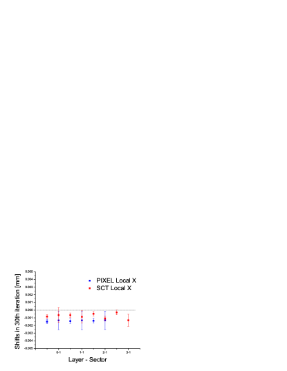
Figure 4: Shifts in the $x$ direction for the 30th iteration of the Robust alignment. Statistical uncertainties on the measurements are represented by the error bars. The quality of the reconstructed track parameters is insensitive to this negligible systematic effect.

3.2 The Valencia approach

The Valencia alignment algorithm [4] is based on the numerical minimization of the $\chi^{2}$ function defined in Eqn. 2 using “biased" residuals (i.e., the hit of the module being aligned is included in the track fit). The covariance matrix is assumed to be diagonal and the diagonal elements are filled with the measurement uncertainties, $\sigma_{r_{i}}$, for residuals, $r_{i}$, both of which are calculated numerically. The only fit parameters are the alignment corrections, ignoring the correlation between track and alignment parameters. The algorithm is therefore executed iteratively, alternating between track and alignment fits.

The SCT endcap outer module strips follow a fan-out geometry and thus have a variable pitch along the vertical direction (Sec. 2). Therefore, instead of using the standard “linear” residual (perpendicular distance from the track prediction to the strip), “angular” residuals ($\delta\gamma$) were used (Fig. 5). These represent the difference between the angular separation of the signal channel and a “fictitious” strip passing through the extrapolated point. The strip-pitch dependence was thus avoided, and uniform angular residuals were obtained.

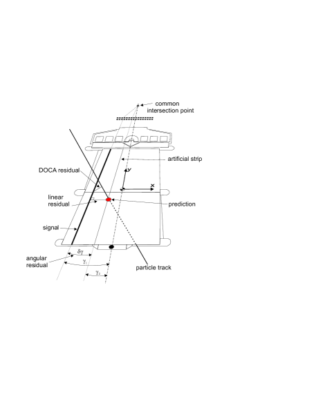
Figure 5: Residual definitions in a SCT end-cap module used by the different alignment algorithms: the angular and linear residuals and distance of closest approach (DOCA).

The outlier hit rejection was applied by defining an acceptance region determined by a critical value of the $\chi^{2}$ (outlier rejection). This value was taken as three standard deviations with respect to the mean value of the reduced residual distribution $(r_{i}/\sigma_{r_{i}})$ calculated before the minimization. The fraction of measurements lying out of the acceptance region was $\sim$3%, and reduced to below 1% if five standard deviations were used.

The Valencia algorithm was intended for runs without magnetic field yielding straight tracks. After reconstruction, each track was extrapolated to the silicon modules. If the extrapolation lay outside the module geometrical acceptance, the track prediction was discarded. The module intersection point of the accepted tracks was transformed into the local frame and residuals were calculated. For Pixels, only measurements in the $\phi$ ($x$) direction were considered. The $\eta$-coordinate was ignored due to the non-Gaussian residual distributions (Fig. 3). For the SCT modules, angular residuals and measurements from both SCT sides were used. Although an analytical residual linearisation as a function of the alignment parameters was not computed, the dependence of the $\chi^{2}$ on the alignment parameters remained linear. Fig. 6 shows the contour regions for two fitted variables and three different confidence level intervals (68%, 90% and 95%) for one Pixel module.

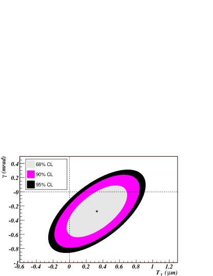
Figure 6: Contour ellipses of constant probability content for three different confidence levels and two alignment parameters of a Pixel module; translation along the most sensitive coordinate (horizontal axis) and tilt angle (vertical axis), as obtained by the Valencia alignment algorithm.

The alignment was performed in three consecutive steps, with variable number of iterations in each step: (st-1) internal alignment of the Pixel modules, (st-2) broad alignment of the SCT modules with respect to the Pixel system, and (st-3) fine alignment of all silicon modules. In st-1 ($\sim$ 6 iterations), tracks lying in the overlap region between Pixel modules in the same layer were selected to enhance the number of overlap hits and to produce a pixel alignment. In st-2 ($\sim$ 2 iterations), tracks reconstructed only with the pixel hits were extrapolated to the SCT planes. In this manner, it was possible to compute SCT residuals (unbiased only in this case) which served as input for an initial alignment of the SCT modules with respect to the Pixel modules. The required correction of the SCT modules was several hundreds of microns. In st-3 ($\sim$ 8 iterations), all silicon modules were included in the track fit and all were aligned simultaneously. In this last stage the alignment corrections per module were of few micrometers.

During alignment, the first Pixel module [layer 0, phi 0] was kept as an anchor; fixed to its nominal position to fix the global degrees of freedom. DoFs to which the sensitivity was very small were excluded from the set of fitted alignment parameters. Module positions along the beam axis were not considered. For Pixels, only the displacements along the sensitive coordinate were fitted. The tilt angle ($\gamma$) was excluded in (st-1 and st-2), but fitted in step (st-3). For the SCT modules, the parameters for displacements along and across the sensitive coordinate together with the in-plane rotation were fitted in all steps. The inclusion of one additional angle ($\beta$) during the last iterations was found to marginally help to improve the results for both sub-detectors.

3.3 The Local $\chi^{2}$ approach

The Local $\chi^{2}$ approach [7, 8] derives from Eqn. 2. The $\chi^{2}$-function uses unbiased residuals, which are defined as the 3D distance of closest approach (Fig. 5). The algorithm uses a diagonal covariance matrix, $V$ that is simlar to that of the Valencia approach. The residual errors are calculated using hit errors and the extrapolated tracking errors.

The Local $\chi^{2}$ algorithm produces alignment constants for each module separately, neglecting correlations between the modules during an iteration. Thus, the solution reduces to inverting as many $N\times N$ matrices as there are modules, where $N$ corresponds to the DoFs of each module (up to 6). Track parameters with a better fit quality gradually bring correlations into play after every iteration.

The fact that CTB was found to be a degenerate setup for track-based alignment required inclusion of external constraints to resolve some of the degeneracies. These were a momentum constraint to the reconstructed tracks and an additional stabilization term to the diagonal elements of the matrix $A$ in Eqn. 3. The stabilization term acts like an additional measurement with a zero residual, full sensitivity in the corresponding degree of freedom (the derivative in Eqn. 3 is equal to one) and an uncertainty $\sigma_{\mathrm{stability}}$. The uncertainty $\sigma_{\mathrm{stability}}$ corresponds to the inverse of the square root of the added term. These additional stability terms constrain the movement to be within $\sigma_{\mathrm{stability}}$. The values for $\sigma_{\mathrm{stability}}$ are 10, 10, 100 $\mu$m for the Pixel $x$,$y$,$z$ coordinates and 100 $\mu$m for the SCT $x$,$y$,$z$ coordinates. For the module rotations the value for $\sigma_{\mathrm{stability}}$ is set to one $mrad$.

The momentum of the incident particles from SPS is known more precisely than the intrinsic momentum resolution of the CTB ID setup. Consequently, this information can be used to constrain the track curvature. Tracks with different beam energies were used as input, using 10,000 events from each pion run listed in Table 1. The alignement procedure was parallelized where multiple jobs with different momentum constraint settings were executed simultaneously. When jobs were finished the alignment information was collected and merged. Subsequently a new iteration with a new set of parallel jobs was started.

The usage of overlap hits, a hit lying in the overlap region of two modules on the same layer, has a profound impact on alignment by constraining relative positions of both sectors, thus avoiding divergences due to lack of external constraints. Residual calculation is also more precise for overlap hits than non-overlap hits. Non-overlap hits were rejected for alignment once a defined limit was reached. In this way the number of overlap hits was enriched with respect to the number of non-overlap hits. The maximum number of non-overlap hits was set to 400.

For the alignment the iteration chain was performed 60 times. The flow of the 6 alignment parameters of each Pixel module through the iterations is shown in Fig. 7. After 10 iterations, nearly all degrees of freedom of all modules converged on stable values. Slower convergence of some parameters was due to the imposed stability term. The procedure was stopped after 60 iterations, when no significant improvement of track parameters was observed and alignment corrections for the sensitive coordinates were at the submicrometer level.

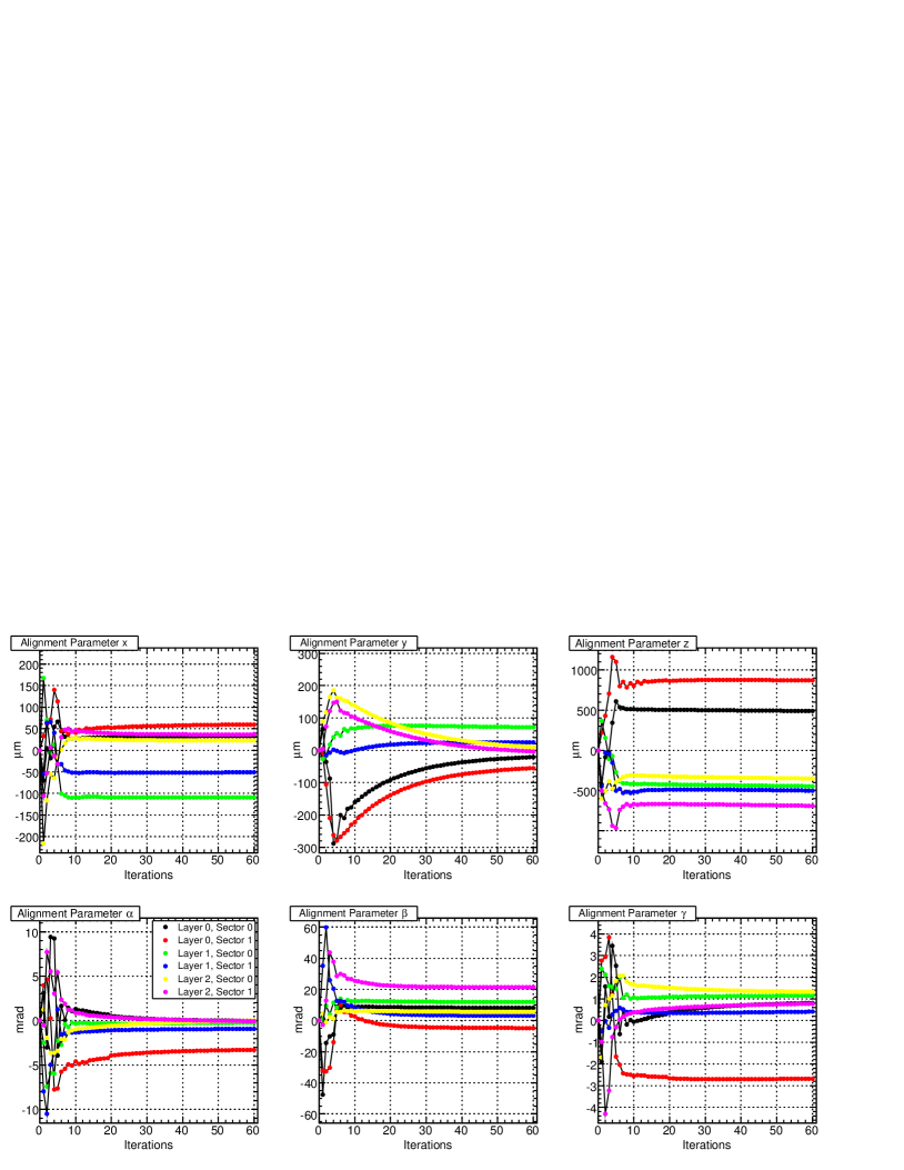
Figure 7: Flow of alignment parameters of the 6 Pixel modules through the iterations of the Local $\chi^{2}$ alignment algorithm.

3.4 The Global $\chi^{2}$ approach

The Global $\chi^{2}$ algorithm [9, 10] is based on the minimization of the $\chi^{2}$ defined as Eqn. 2 with respect to the alignment parameters. The residuals are defined within the module plane and are biased (i.e., the hit of the module being aligned is included in the track fit). They depend on the track parameters ($\pi$) as well as on the subset of alignment parameters related to the intersected module ($\mathbf{a}$):

$$\frac{d\mathbf{r}}{d\mathbf{a}}=\frac{\partial\mathbf{r}}{\partial\mathbf{a}}+\frac{\partial\mathbf{r}}{\partial\mbox{\boldmath$\pi$}}\frac{d\mbox{\boldmath$\pi$}}{d\mathbf{a}}~{}.$$ (8)

The method has the advantage of properly treating all correlations between residuals arising from common track parameters and Multiple Coulomb Scattering (MCS). Solution 3 requires inverting a symmetric matrix of size $N\times N$, where $N$ is the number of DoFs of the problem. For large systems (for instance, the entire ATLAS ID), the solution with accurate numerical precision and in a reasonable CPU time could be a challenge [24]. In the CTB case, however, the system consisted of just 14 silicon modules. Therefore it was free from such numerical limitations. Intrinsic alignment of an unconstrained system always leads to a singular matrix and consequently an ill-defined solution. This is best solved by diagonalization of the matrix. The singular modes can subsequently be ignored in the solution. The procedure can be further extended to remove all “weak modes” which either represent unphysical deformations or have an associated error exceeding expected misalignments.

In order to solve the CTB alignment, the following approach was adopted: two anchor modules were chosen (the first Pixel and the last SCT) which removed the exact singularities from the solution. All considered tracks were nearly parallel to one another and orthogonal to the SCT module planes. Also the $y$ tilt angles of the Pixel modules were considered to be very accurately known from the survey. Consequently the following DoFs were removed from the fit: out of the plane translation and the rotations with respect to $x$ and $y$-axes. This choice resulted in 3 DoFs per module (36 in total). However, results indicated a substantial residual misalignment related to the uncorrected $y$ rotation of the Pixel modules. The largest misalignment was found for the upper module in layer 2 with a value of $25.2\pm 0.5~{}mrad$. The $y$ rotations of the Pixel modules were eventually included in the alignment fit which efficiently eliminated the corresponding misalignments.

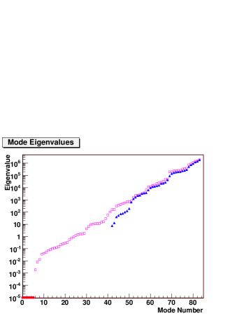
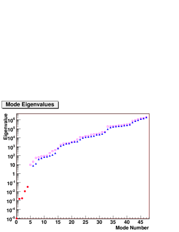
Figure 8: Left: original eigenspectrum of the unconstrained solution (84 DoFs - open squares) overlaid with that of the actual solution (42 DoFs - solid triangles) of Global $\chi^{2}$ algorithm. Six solid circles on the leftmost are the singular modes of the asymptotic freedom of the system. Their actual value is zero up to the numerical precision and were fixed to $10^{-5}$ for clarity only. Right: actual solution eigenspectrum (42 DoFs - solid triangles) compared to the analogous one without the anchor modules requirement (open squares). The five solid circles are the new near-singularities.

The final alignment was concerned with 42 DoFs. Fig. 8 shows the comparison of eigenspectra (obtained by DSPEV routine from the LAPACK library [25]) of the unconstrained CTB geometry and the one used for the final alignment. Elimination of unphysical parameters efficiently removed the lowest part of the eigenspectrum. Fig. 8 gives also the comparison of the final alignment to the one without anchor modules. The five weak modes correspond to the approximate freedom of two global translations and three rotations of the entire setup.

The method required four iterations for convergence, however a total of seven iterations was used on about 50,000 events at each iteration. Translations of some SCT modules in $y$-direction were found to be as large as 1.5 mm; $x$ translations never exceeded 0.4 mm.

4 Results

In order to assess the quality of the alignment, one must check the track reconstruction quality and physics observables. For this purpose, the alignment corrections were applied to the data detailed in Table 1.

After aligning the modules, the track finding efficiency increased. For example, for the Robust alignment approach, the number of tracks per event was found to stabilize at around 0.95. As expected, an average of three hits in the pixels and eight in the SCT (two per module) were found. All four alignment approaches produced similar performances, consistent with the simulation.

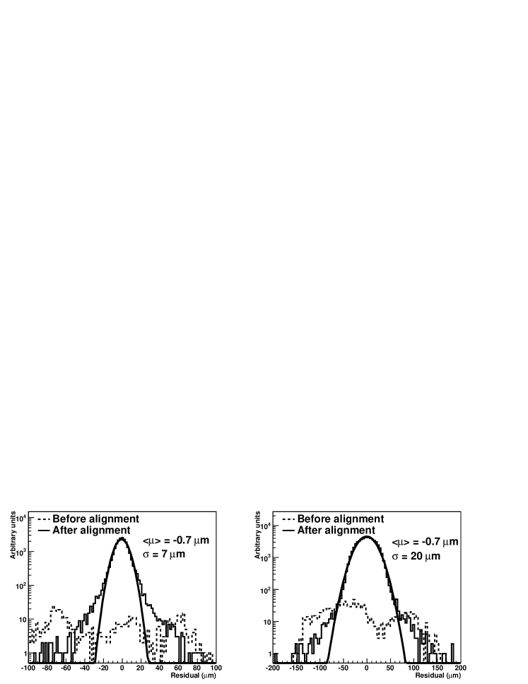
Figure 9: Residuals of all Pixels (left) and all SCT (right) modules before and after alignment. The width of the distribution is consistent with the intrinsic resolution of the modules.

A well-aligned setup returns residuals with a mean of zero and a width consistent with the intrinsic resolution of the detector and the track fit errors. Fig. 9 shows the biased $x$-residuals of all the Pixel and SCT modules for the 100 GeV pion run, for those tracks which had at least three pixel and six SCT hits. The width of the distribution after alignment is consistent with the intrinsic resolution of Pixels and SCT modules. Fig. 10 shows the mean of Pixel module residuals for an example run (20 GeV/c pion run). While simulation residual means are centered around zero for all modules, the aligned detector data show fluctuations. From the size of the fluctuations, we conclude that the Pixel residuals of all alignment methods agree within $5~{}\mu m$ over the whole momentum range. Fig. 10 also shows a good agreement between the $\chi^{2}$ minimization methods and the simulation on the residual resolutions. The Robust method results in a worse residual resolution since this method only corrects for alignment shifts in the module plane. Fig. 10 also reveals a dependence of the $\sigma$ of the pixel residuals on the module number. This indicates contributions to the resolution from the geometry of the setup in addition to the intrinsic detector resolution. The residuals also vary because the track error varies along the track due to MCS, for example.

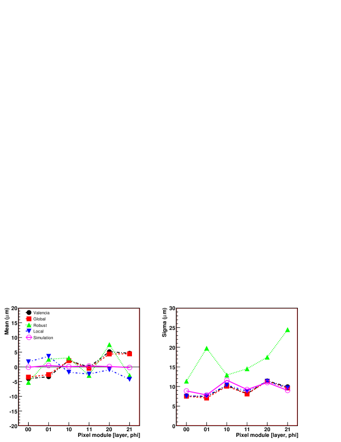
Figure 10: Pixel biased $\phi$-residuals mean (left) and $\sigma$ (right) distributions for the aligned data and the simulation, for the 20 GeV pion run with B=1.4 T.

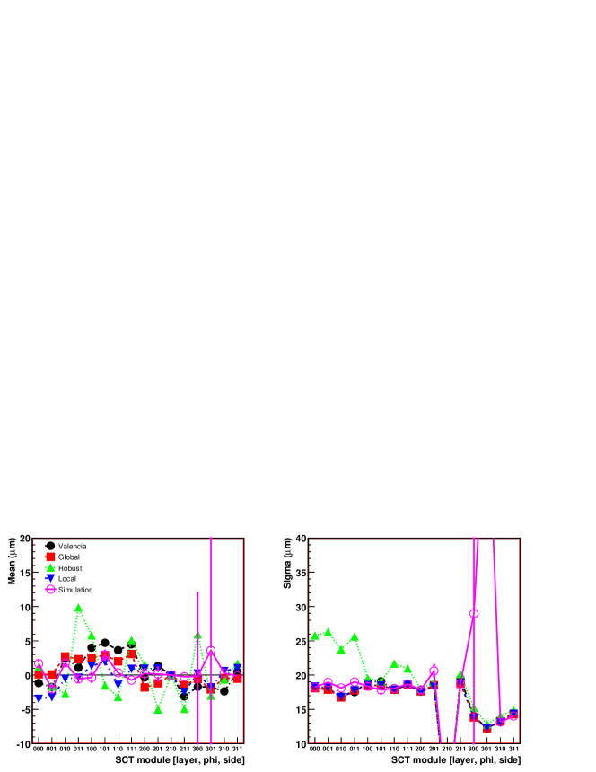
Figure 11: SCT biased residuals mean (left) and $\sigma$ (right) distributions for the aligned data and the simulation, for a 20 GeV pion run with B=1.4 T. A single SCT module has two entries in each plot (e.g. 000 and 001 correspond, respectively, to the module front and back plane at layer 0, sector 0). The dip at index 210 in the right plot corresponds to the plane which was not working.

The residual mean distributions for each SCT plane are shown in Fig. 11. Systematic correlations in the signs of the means is observed among the alignment algorithm results. Fig. 11 also shows that the residual resolution of the SCT modules in aligned data (except those reconstructed using Robust method alignment corrections) are around 20 $\mu m$, which is in good agreement with the simulation.

All track parameters at the perigee ($d_{0}$, $z_{0}$, $\phi_{0}$ and $\theta_{0}$ and the momentum) were examined when tracks were reconstructed with the alignment corrections from the four algorithms. The values of spatial track parameters were not exactly similar for tracks reconstructed with different constants, however, they followed consistent trends for the runs studied. The difference can be attributed to the insufficiently constrained global degrees of freedom. The residuals and curvature, hence the track fit $\chi^{2}$ and the $p_{T}$, are invariant under rigid body translations and rotations of the whole system.

The reconstructed $\phi_{0}$ and $\theta_{0}$ values depend on the beam properties as well as the module locations provided by the algorithms. Therefore, the measured $\phi_{0}$ and $\theta_{0}$ in data were used to tune the beam spread in the simulation and to evaluate the interaction length, $X_{0}$, upstream of the CTB setup. The track $\phi_{0}$ and $\theta_{0}$ resolutions improved with increasing momentum, as expected with a reduced MCS for more energetic particles.

The momentum reconstruction provides a very powerful test of the alignment performance. Fig. 12 shows the recovery of the momentum resolution of the 100 GeV pion run after alignment, from a highly degraded initial measurement. The momentum measurement does not depend on global transformations. Therefore the momenta of the tracks reconstructed with different alignment constants ought to agree. Fig. 13 is used to compare the electron and pion momenta resolution as a function of the reconstructed momentum obtained from the four alignment methods to the simulation. The momenta reconstructed using all algorithms, in particular $\chi^{2}$ minimization ones, are consistent with the simulation. The Robust method returns slightly worse results since the alignment does not take rotations of the modules into account.

The reconstructed electron momentum is significantly less than the nominal (set by the beamline), for both data and simulation. The presence of several layers of upstream material can account for this effect, because the radiated energy of electrons before they enter the tracking volume was not recovered. As pions do not suffer as much from energy loss, their reconstructed momenta agree much better with the nominal set by the SPS.

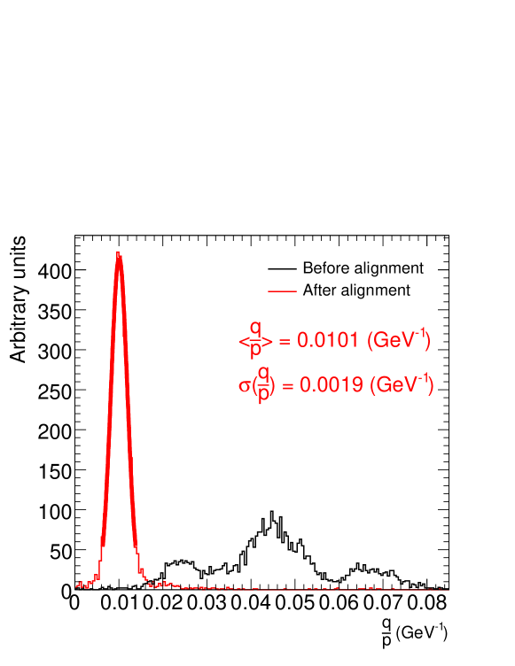
Figure 12: Momentum resolution of Pixel and SCT detectors for a 100 GeV pion run with non-zero B-field with and without alignment corrections.

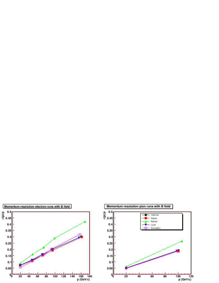
Figure 13: Momentum resolution as a function of the reconstructed momentum.

The convergence of alignment corrections per iteration and the improved residual distributions presented are mandatory but not sufficient to ensure the success of the alignment. Unfortunately, survey data of the CTB detector setup does not exist, therefore, a comparison with the derived alignment sets was not possible. However, a comparison of the position and orientation of each detector element derived with the four algorithms served as a means of validation.

When the alignment constants for the four algorithms were compared, the algorithms were observed to provided large corrections (several hundred microns). The chosen alignment strategy (fixing one or several modules as opposed to leaving the whole system free floating or constraining or removing some DoFs from the alignment) has an impact on the solution of the global DoF of the system. In order to compare the results of the different algorithms, they need to be globally matched. Allowing a global offset for each alignment set was chosen to be the method of finding a best match of the alignment results. After having subtracted the global offsets between the geometries, it was observed that a good agreement between the algorithms for the most sensitive coordinates $x$, $y$ and $\gamma$ was reached. Given the low sensitivity of the alignment procedures to the alpha and beta rotations, the agreement between the algorithms for these coordinates was only marginally improved.

5 Summary and Conclusion

Four independent algorithms were used to successfully align the setup formed by the silicon modules of the ATLAS Inner Detector tracker, using data collected during the 2004 Combined Test Beam. The reconstructed track parameters and hit residual distributions were studied. The performance of the alignment algorithms was assessed by comparing with a simulation, in which all modules were at their nominal positions. The simulation can be taken as a benchmark where all errors were regarded as only being due to the intrinsic resolution of the modules.

All alignment approaches yielded results for the reconstructed momentum of electrons and pions that agreed with the simulation. Slightly worse momentum resolution was observed using the Robust algorithm. This was understood and explained by the fact that the algorithm was limited to re-alignment of the two in-plane translations only. The unresolved residual misalignments (e.g. in-plane rotations) unavoidably led to reduced track fit quality and consequently increased uncertainties on the reconstructed curvature. For the remaining track perigee parameters, consistent results were obtained with each method.

All four methods agree well on the residuals for all modules and planes, and with the simulation. The resolution of individual pixel modules is around 10 $\mu$m and the SCT around 20 $\mu$m. Observed differences for the residual mean values remain below 5 $\mu$m. We conclude that the silicon modules of the ATLAS ID were aligned at the CTB with a precision of 5 $\mu$m in their most precise coordinate.

The data collected at the ATLAS Combined Test Beam in 2004 served as an invaluable test bed for the Inner Detector alignment algorithms. For the first time ever, the readiness of the alignment algorithms was assessed with experimental data. All algorithms performed satisfactorily given the limitations inherent to the CTB geometry and the beamline arrangement. The narrow tower of modules and almost parallel particle beams gave rise to undetermined degrees of freedom. These were successfully dealt with by the four algorithms, each in its own way, providing consistent and high quality measurements of the test beam track parameters.

- [1] ATLAS Collaboration, ATLAS Inner Detector, Technical Design Report Volume 1, in ATLAS TDR 4, (CERN/LHCC 97-16, 1997)
- [2] ATLAS Collaboration, The ATLAS Computing Technical Design Report Volume, CERN-LHCC-2005-022, 2005
- [3] T. Cornelissen, Track fitting in the ATLAS experiment, Ph.D. thesis, Universiteit van Amsterdam (Netherlands), 2006
- [4] S. Gonzalez-Sevilla, ATLAS Inner Detector performance and alignment studies, Ph.D. thesis, Universitat de Valencia (Spain), 2007
- [5] F. Campabadal et al., Nucl. Inst. and Meth. A538 (2005)
- [6] F. Heinemann, Robust Track Based Alignment of the ATLAS Silicon Detector and Assessing Parton Distribution Uncertainties in Drell-Yan Processes, Ph.D. thesis, University of Oxford, 2007
- [7] R. Härtel, Iterative local alignment approach for the ATLAS SCT detector, Diploma thesis, TU München, 2005, MPP-2005-174
- [8] T. Göttfert, Iterative local alignment algorithm for the ATLAS Pixel detector, Diploma thesis, Universität Würzburg, 2006, MPP-2006-118
- [9] P. Bruckman de Renstrom, A. Hicheur, S. Haywood, Global approach to the alignment of the ATLAS silicon tracking detectors, ATL-INDET-2005-002, 2004
- [10] A. Hicheur and S. Gonzalez-Sevilla, Implementation of a global fit method for the alignment ot the silicon tracker in Athena framework, CHEP 06, Mumbai, India, 2006
- [11] S. Blusk (ed.) et al., Proceedings of the first LHC Detector Alignment Workshop, CERN, 2006
- [12] B.D. Girolamo, M. Gallas and T. Koffas, ATLAS Barrel Combined Run in 2004, Test Beam Setup and its evolutions, CERN EDMS Public Note: ATC-TT-IN-0001, 2005
- [13] I. Gorelov, Int. J. Mod. Phys. A16S1C (2001) 1100–1102
- [14] C. Gemme, Nucl. Instrum. Meth. A501 (2003) 87–92
- [15] L. Blanquart et al., IEEE Trans. Nucl. Sci. 51 (2004) 1358–1364
- [16] A. Ahmad et al., Nucl. Instrum. Meth. A578 (2007) 98–118
- [17] A. Abdesselam et al., Nucl. Instrum. Meth. A575 (2007) 353–389
- [18] W. Dabrowski et al., IEEE Trans. Nucl. Sci. 47 (2000) 1843–1850
- [19] B.D. Girolamo et al., Beamline instrumentation in the 2004 combined ATLAS testbeam, ATL-TECH-PUB-2005-001, 2005
- [20] S. Gadomski et al., IEEE Trans. Nucl. Sci. 53 (2006)
- [21] G. Lutz, Nucl. Instrum. Meth. A273 (1988) 349–361
- [22] G. Gorfine et al., Nucl. Inst. and Meth. A565 (2006), Proceedings of Pixel2005
- [23] L. Lonnblad, Comput. Phys. Commun. 84 (1994) 307–316
- [24] M. Karagöz Ünel et al., Parallel computing studies for the alignment of the ATLAS silicon tracker, CHEP 06, Mumbai, India, 2006
- [25] E. Anderson et al., LAPACK Users’ Guide, http://netlib.org/lapack/lug, 1999.