TUM-HEP 687/08

Running minimal flavor violation

Paride Paradisi, Michael Ratz, Roland Schieren, Cristoforo Simonetto

Physik-Department T30/T31, Technische Universität München,
James-Franck-Straße, 85748 Garching, Germany

We consider the flavor structure of the minimal supersymmetric standard model (MSSM) in the framework of ‘minimal flavor violation’ (MFV). We show that, if one imposes the MFV structure at some scale, to a good accuracy the MFV decomposition works at all other scales. That is, quantum effects can be described by running coefficients of the MFV decomposition. We find that the coefficients get driven to non-trivial fixed points.

1 Introduction

Despite of its great phenomenological success, the standard model (SM) is certainly not completely satisfactory from a theoretical point of view. Certain aspects of the SM hint at unified structures: the gauge interactions and the quantum numbers of the fundamental fermions fit nicely into the framework of a grand unified theories (GUTs). As is well known, GUTs seem to require low-energy supersymmetry, as this most allows for the compelling scenarios of gauge unification. This leads to the picture of the so-called ‘SUSY desert’, i.e. between the TeV scale and the GUT scale no new physics appears. On the other hand, attempts to find a simple explanation of the SM flavor structure have not yet been as successful as one could have hoped.

In this study we consider the minimal supersymmetric extension of the SM (MSSM), where the flavor structure is particularly rich because of the various additional soft terms. As is well known, the flavor parameters are tightly constrained by phenomenology, leading to what is usually called the supersymmetric flavor problems. These problems may be viewed as evidence against low-energy supersymmetry. Adopting a more optimistic point of view, one could say that the non-observation of certain flavor transitions enforces a rather special form of soft terms, so that one can gain additional insights on the origin of flavor by studying superpartner interactions.

An efficient way to ameliorate (or even avoid) the supersymmetric flavor problems is to assume that the (soft) masses of the squarks and sleptons, i.e. the scalar superpartners of SM quarks and leptons, are close to a unit matrix. In this case the super-GIM mechanism is at work [1], i.e. unobserved flavor transitions are strongly suppressed. It has been rather popular to assume that soft masses are proportional to the unit masses at a high scale, such as the GUT scale, and all deviations come from radiative corrections, induced by the Yukawa couplings. However, one might argue that this assumption lacks a fundamental motivation.

In this note, we consider a slightly modified setting in which this strong assumption gets somewhat relaxed. We shall assume that at the GUT scale the scalar soft mass squareds receive corrections that are proportional to $\boldsymbol{Y}^{\dagger}\boldsymbol{Y}$ where $\boldsymbol{Y}$ denotes a Yukawa coupling matrix. In other words, we study the implications of an ansatz which is known as ‘minimal flavor violation’ (MFV) [2, 3, 4] at the GUT scale.

2 A short review of the MFV ansatz

As is well known, the MFV ansatz is motivated as follows: in the limit of vanishing Yukawa couplings the MSSM enjoys an enhanced (classical) symmetry,

$$G_{\mathrm{flavor}}~{}=~{}\mathrm{SU}(3)_{u}\times\mathrm{SU}(3)_{d}\times\mathrm{SU}(3)_{Q}\times\mathrm{SU}(3)_{e}\times\mathrm{SU}(3)_{L}\;.$$ (1)

One might then view the Yukawas as vacuum expectation values (vevs) of ‘spurion’ fields. If these spurions are the only source of flavor violation, this implies that any operator not respecting $G_{\mathrm{flavor}}$ has to be proportional to the spurions, i.e. to the Yukawas. This then leads to the following expansion of soft supersymmetry breaking operators [4]:

$$\boldsymbol{m}_{Q}^{2} = \alpha_{1}\,\mathds{1}+\beta_{1}\,\boldsymbol{Y}_{\!\!u}^{\dagger}\boldsymbol{Y}_{\!\!u}+\beta_{2}\,\boldsymbol{Y}_{\!\!d}^{\dagger}\boldsymbol{Y}_{\!\!d}+\beta_{3}\,\boldsymbol{Y}_{\!\!d}^{\dagger}\boldsymbol{Y}_{\!\!d}\,\boldsymbol{Y}_{\!\!u}^{\dagger}\boldsymbol{Y}_{\!\!u}+\beta_{3}\,\boldsymbol{Y}_{\!\!u}^{\dagger}\boldsymbol{Y}_{\!\!u}\,\boldsymbol{Y}_{\!\!d}^{\dagger}\boldsymbol{Y}_{\!\!d}\;,$$ (2a)

$$\boldsymbol{m}_{u}^{2} = \alpha_{2}\,\mathds{1}+\beta_{5}\,\boldsymbol{Y}_{\!\!u}\boldsymbol{Y}_{\!\!u}^{\dagger}\;,$$ (2b)

$$\boldsymbol{m}_{d}^{2} = \alpha_{3}\,\mathds{1}+\beta_{6}\,\boldsymbol{Y}_{\!\!d}\boldsymbol{Y}_{\!\!d}^{\dagger}\;,$$ (2c)

$$\boldsymbol{A}_{u} = \alpha_{4}\,\boldsymbol{Y}_{\!\!u}+\beta_{7}\,\boldsymbol{Y}_{\!\!u}\,\boldsymbol{Y}_{\!\!d}^{\dagger}\boldsymbol{Y}_{\!\!d}\;,$$ (2d)

$$\boldsymbol{A}_{d} = \alpha_{5}\,\boldsymbol{Y}_{\!\!d}+\beta_{8}\,\boldsymbol{Y}_{\!\!d}\,\boldsymbol{Y}_{\!\!u}^{\dagger}\boldsymbol{Y}_{\!\!u}\;,$$ (2e)

$$\boldsymbol{A}_{e} = \alpha_{e}\,\boldsymbol{Y}_{\!\!e}\;.$$ (2f)

Higher order terms in this expansion can be neglected due to the Yukawa hierarchies. Note that our notation is slightly different from the one used in [4] in that our coefficients $\alpha_{i}$ and $\beta_{i}$ carry mass dimension. This is done in order to simplify the expressions to be presented below. In our notation of Yukawa couplings and scalar soft mass squareds we follow [5].

As discussed above, the MFV ansatz offers a natural way to avoid unobserved large effects in flavor physics. However, we would like to stress here that small departures from complete flavor blindness of the soft terms can still provide interesting effects in low energy processes. In particular, the $\beta_{1}\,\boldsymbol{Y}_{\!\!u}^{\dagger}\boldsymbol{Y}_{\!\!u}$ term in $\boldsymbol{m}_{Q}^{2}$ induces Flavor Changing Neutral Currents (FCNC) phenomena, such as $B\to X_{s}\gamma$, through a loop exchange of gluinos and squarks. For $\mathcal{O}(1)$ values of the MFV parameter $\beta_{1}$, sizable or even dangerous contributions to flavor physics observables can be expected, depending on the absolute soft SUSY scale. Additionally, from a phenomenological side, it is well known that both FCNC transitions and the prediction for the lightest Higgs boson mass are highly sensitive to the $\boldsymbol{A}_{u}$ term in the stop sector thus, the MFV modifications to $\boldsymbol{A}_{u}$ can play, in principle, a relevant role. In this respect, one might expect that low-energy observables can still represent a useful tool to test and/or constrain the MFV parameters at the high scale. In particular, one would expect to find departures from the predictions of mSUGRA models where a completely flavor blind scenario is realized at the high scale. However, as we will discuss in the next sections, this is not the case.

3 MFV decomposition and renormalization effects

3.1 Scale-independent validity of the MFV ansatz

Usually the MFV ansatz is imposed at a scale close to the electroweak scale. As mentioned in the introduction, we will be interested in the situation where it is imposed at the GUT scale. Since the spurion argument does not imply a preferred scale, one might expect that, if the MFV decomposition applies at one renormalization scale, it will apply at different scales as well. That is, renormalization effects will modify the values of the coefficients, $\alpha_{i}$ and $\beta_{i}$, but not the validity of the ansatz.

We have checked explicitly that this is the case: we start with soft terms complying with the decomposition (2) at the GUT scale and run them down to the SUSY scale, i.e. solve the corresponding renormalization group equations (RGEs). Then we successfully fit the low energy soft masses by the decomposition (2), i.e. when inserting the Yukawa matrices at the low scale we find values of the MFV parameters $\alpha_{i}$ and $\beta_{i}$ such that the mass matrices are reproduced with a high accuracy. The details of our numerical studies are deferred to appendix A.

3.2 RGEs for the MFV parameters

Having seen that the running of the soft masses can described in terms of scale dependent MFV coefficients $\alpha_{i}$ and $\beta_{i}$ we now study the behavior of these coefficients under the renormalization group. We calculate the RGEs for the $\alpha_{i}$ and $\beta_{i}$ by inserting (2) in the one-loop RGEs for the soft-masses and the trilinear couplings (cf. [5]). Note that there are two sources for the running of the MFV coefficients: first, the soft terms run, and second, the Yukawa matrices, to which we match the soft terms, also depend on the renormalization scale. Neglecting the Yukawa couplings of the first and second generation, the results read

$$16\pi^{2}\frac{\text{d}\alpha_{1}}{\text{d}t} = -\frac{32}{3}g_{3}^{2}|M_{3}|^{2}-6g_{2}^{2}|M_{2}|^{2}-\frac{2}{15}g_{1}^{2}|M_{1}|^{2}+\frac{1}{5}g_{1}^{2}S\;,$$ (3a)

$$16\pi^{2}\frac{\text{d}\alpha_{2}}{\text{d}t} = -\frac{32}{3}g_{3}^{2}|M_{3}|^{2}-\frac{32}{15}g_{1}^{2}|M_{1}|^{2}-\frac{4}{5}g_{1}^{2}S\;,$$ (3b)

$$16\pi^{2}\frac{\text{d}\alpha_{3}}{\text{d}t} = -\frac{32}{3}g_{3}^{2}|M_{3}|^{2}-\frac{8}{15}g_{1}^{2}|M_{1}|^{2}+\frac{2}{5}g_{1}^{2}S\;,$$ (3c)

$$16\pi^{2}\frac{\text{d}\alpha_{4}}{\text{d}t} = 12\alpha_{4}y_{t}^{2}+10\beta_{7}y_{t}^{2}y_{b}^{2}+2\beta_{8}y_{t}^{2}y_{b}^{2}+\frac{32}{3}g_{3}^{2}M_{3}+6g_{2}^{2}M_{2}+\frac{26}{15}g_{1}^{2}M_{1}\;,$$ (3d)

$$16\pi^{2}\frac{\text{d}\alpha_{5}}{\text{d}t} = 12\alpha_{5}y_{b}^{2}+10\beta_{8}y_{t}^{2}y_{b}^{2}+2\beta_{7}y_{t}^{2}y_{b}^{2}+\frac{32}{3}g_{3}^{2}M_{3}+6g_{2}^{2}M_{2}+\frac{14}{15}g_{1}^{2}M_{1}+2\alpha_{e}y_{\tau}^{2}\;,$$

$$16\pi^{2}\frac{\text{d}\beta_{1}}{\text{d}t} = 2m_{H_{u}}^{2}+2\alpha_{4}^{2}+2\beta_{8}^{2}y_{t}^{2}y_{b}^{2}+2\alpha_{1}+2\alpha_{2}$$ (3f)

$${}-10\beta_{1}y_{t}^{2}+2\beta_{5}y_{t}^{2}+\beta_{1}\left(\frac{32}{3}g_{3}^{2}+6g_{2}^{2}+\frac{26}{15}g_{1}^{2}\right)\;,$$

$$16\pi^{2}\frac{\text{d}\beta_{2}}{\text{d}t} = 2m_{H_{d}}^{2}+2\alpha_{5}^{2}+2\beta_{7}^{2}y_{t}^{2}y_{b}^{2}+2\alpha_{1}+2\alpha_{3}-10\beta_{2}y_{b}^{2}-2\beta_{2}y_{\tau}^{2}+2\beta_{6}y_{b}^{2}$$ (3g)

$${}+\beta_{2}\left(\frac{32}{3}g_{3}^{2}+6g_{2}^{2}+\frac{14}{15}g_{1}^{2}\right)\;,$$

$$16\pi^{2}\frac{\text{d}\beta_{3}}{\text{d}t} = 2\alpha_{4}\beta_{7}+2\alpha_{5}\beta_{8}-12\beta_{3}y_{t}^{2}-12\beta_{3}y_{b}^{2}-2\beta_{3}y_{\tau}^{2}+\beta_{3}\left(\frac{64}{3}g_{3}^{2}+12g_{2}^{2}+\frac{8}{3}g_{1}^{2}\right)\;,$$

$$16\pi^{2}\frac{\text{d}\beta_{5}}{\text{d}t} = 4m_{H_{u}}^{2}+4\left(\alpha_{4}+\beta_{7}y_{b}^{2}\right)^{2}+4\alpha_{1}+4\alpha_{2}+4\beta_{1}y_{t}^{2}+4\beta_{2}y_{b}^{2}+8\beta_{3}y_{t}^{2}y_{b}^{2}$$ (3i)

$${}+\beta_{5}\left(-8y_{t}^{2}-2y_{b}^{2}+\frac{32}{3}g_{3}^{2}+6g_{2}^{2}+\frac{26}{15}g_{1}^{2}\right)\;,$$

$$16\pi^{2}\frac{\text{d}\beta_{6}}{\text{d}t} = 4m_{H_{d}}^{2}+4\left(\alpha_{5}+\beta_{8}y_{t}^{2}\right)^{2}+4\alpha_{1}+4\alpha_{3}+4\beta_{1}y_{t}^{2}+4\beta_{2}y_{b}^{2}+8\beta_{3}y_{t}^{2}y_{b}^{2}$$ (3j)

$${}+\beta_{6}\left(-2y_{t}^{2}-8y_{b}^{2}-2y_{\tau}^{2}+\frac{32}{3}g_{3}^{2}+6g_{2}^{2}+\frac{14}{15}g_{1}^{2}\right)\;,$$

$$16\pi^{2}\frac{\text{d}\beta_{7}}{\text{d}t} = 2\alpha_{5}+\beta_{7}\left(-12y_{b}^{2}-2y_{\tau}^{2}+\frac{32}{3}g_{3}^{2}+6g_{2}^{2}+\frac{14}{15}g_{1}^{2}\right)\;,$$ (3k)

$$16\pi^{2}\frac{\text{d}\beta_{8}}{\text{d}t} = 2\alpha_{4}+\beta_{8}\left(-12y_{t}^{2}+\frac{32}{3}g_{3}^{2}+6g_{2}^{2}+\frac{26}{15}g_{1}^{2}\right)\;.$$ (3l)

Here $\text{d}/\text{d}t$ denotes the logarithmic derivative w.r.t. the renormalization scale, $g_{1}$, $g_{2}$, $g_{3}$ are the gauge couplings, $M_{1}$, $M_{2}$, $M_{3}$ the gaugino masses, $y_{t}$, $y_{b}$, $y_{\tau}$ the third family Yukawa couplings, $m_{H_{u}}$, $m_{H_{d}}$ the Higgs soft mass terms. We have further defined

$$S = m_{H_{u}}^{2}-m_{H_{d}}^{2}+\mathrm{Tr}\bigg{[}\alpha_{1}\mathds{1}+\beta_{1}\boldsymbol{Y}_{\!\!u}^{\dagger}\boldsymbol{Y}_{\!\!u}+\beta_{2}\boldsymbol{Y}_{\!\!d}^{\dagger}\boldsymbol{Y}_{\!\!d}+2\beta_{3}\boldsymbol{Y}_{\!\!d}^{\dagger}\boldsymbol{Y}_{\!\!d}\boldsymbol{Y}_{\!\!u}^{\dagger}\boldsymbol{Y}_{\!\!u}$$ (4)

$${}-2\alpha_{2}\mathds{1}-2\beta_{5}\boldsymbol{Y}_{\!\!u}\boldsymbol{Y}_{\!\!u}^{\dagger}+\alpha_{3}\mathds{1}+\beta_{6}\boldsymbol{Y}_{\!\!d}\boldsymbol{Y}_{\!\!d}^{\dagger}-\boldsymbol{m}_{L}^{2}+\boldsymbol{m}_{e}^{2}\bigg{]}$$

with $\boldsymbol{m}_{L}^{2}$ and $\boldsymbol{m}_{e}^{2}$ denoting the $3\times 3$ mass matrices for the charged lepton doublets and singlets, respectively.

3.3 Approximations of low-energy MFV coefficients

We derive approximate relations between the values at the GUT scale and the low scale. Here we assume mSUGRA inspired initial conditions (for details see equation (9) in appendix B) and allow for one non-zero $\beta_{i}$ while the others are set to zero. The value of $\tan\beta$ is fixed to 10. The formulae are obtained by varying the initial values of $m_{\nicefrac{{1}}{{2}}},m_{0},A,\beta_{i}$, running them down to the low scale and fitting a linear combination of the parameters to the obtained points in parameter-space. Details and the results are shown in appendix B.

3.4 Fixed points in the evolution of the MFV coefficients

Let us now come to the discussion of the relation between the boundary values for the MFV coefficients at the high scale and the values they attain at the low scale. A crucial feature of the low-energy values of the MFV coefficients $\beta_{i}$ is that they are rather insensitive to their GUT boundary values. It is, of course, well known that the soft masses tend to get aligned due to the renormalization group evolution [6, 7, 8, 9]. Our results make this statement more precise. There is an on-going competition between the alignment process, triggered mainly by the positive gluino contributions, and misalignment process, driven by negative effects proportional to the Yukawa matrices. These effects are so strong that the memory to the initial conditions gets almost wiped out, at least as long as the ratio between scalar and gaugino masses at the high scale is not too large.

To illustrate the behavior under the renormalization group, we analyze the situation at several benchmark points. These points were chosen to be the so-called SPS points [10] (cf. table 1) amended by corrections in the MFV form.

Point $m_{0}$ $m_{\nicefrac{{1}}{{2}}}$ $A$ $\tan\beta$ 1a 100 GeV 250 GeV -100 GeV 10 1b 200 GeV 400 GeV 0 30 2 1450 GeV 300 GeV 0 10 3 90 GeV 400 GeV 0 10 4 400 GeV 300 GeV 0 10 5 150 GeV 300 GeV -1000 GeV 5

Table 1: Survey of SPS points.

Examples for the RG behavior are displayed in figures 1 and 2. We show the ratio $\beta_{1}/\alpha_{1}$ and $\beta_{6}/\alpha_{3}$, respectively. Note that these ratios coincide with $b_{1}/a_{1}$ and $b_{6}/a_{3}$ in the original MFV decomposition [4]. These ratios parametrize the deviations of the soft terms from unit matrices. In our illustrations, we use two different initial conditions for the $\beta_{i}$. For the solid curve only the shown parameter is set non-zero at the high scale, i.e. in figure 1 only $\beta_{1}$ has a non-zero initial value, while the dashed curves correspond to universal initial conditions for the $\beta_{i}$. That is, we choose input values of the soft terms of the form (2) with

$$\alpha_{i}~{}=~{}m_{0}^{2}\quad\text{and}\quad\beta_{j}=0~{}\forall j\neq k\quad\text{or}\quad\beta_{i}~{}=~{}\text{universal}\;.$$ (5)

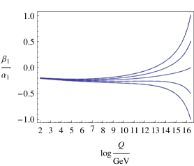
(a) SPS1a

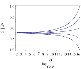
(b) SPS1b

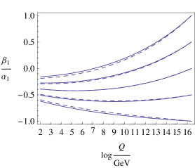
(c) SPS2

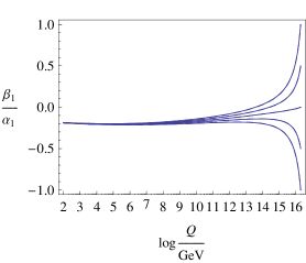
(d) SPS3

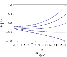
(e) SPS4

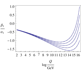
(f) SPS5

Figure 1: The running of $\frac{\beta_{1}}{\alpha_{1}}$. For the solid curve only $\beta_{1}$ is non-zero at the high scale while for the dashed curve all $\beta_{i}$ are switched on.

(a) SPS1a

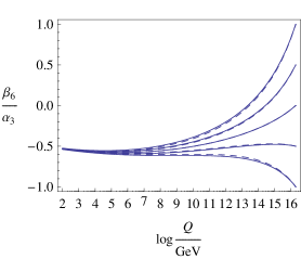
(b) SPS1b

(c) SPS2

(d) SPS3

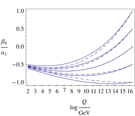
(e) SPS4

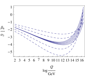
(f) SPS5

Figure 2: The running of $\frac{\beta_{6}}{\alpha_{3}}$. For the solid curve only $\beta_{6}$ is non-zero at the high scale while for the dashed curve all $\beta_{i}$ are switched on.

We observe that the ratios get driven to non-trivial, i.e. non-zero, fixed points. The corresponding low-energy fixed point values can be inferred from our numerical approximations in appendix B. These fixed points emerge from the competition from alignment and misalignment processes, as discussed above.

4 Beyond MFV

The MFV ansatz is usually justified by a spurion argument. However, there are some drawbacks to this reasoning. First of all, $G_{\mathrm{flavor}}$ (cf. equation (1)) is anomalous. Secondly, it is hardly conceivable that one (spurion) field vev can give rise to a rank three Yukawa coupling with hierarchical eigenvalues. From these considerations we infer that the flavor symmetry will likely be broken by more than one field, such that Yukawa couplings and corrections to soft parameters are proportional to linear combinations of such fields with, in general, different coefficients. In this picture one would expect corrections to the MFV scheme.

Assuming that both new physics interactions and flavor models operate at the high scale, it is worthwhile to understand the implications of the presence of non-MFV terms $\boldsymbol{\Delta m}^{2}_{f},\boldsymbol{\Delta A}_{f}$, which we add to the ansatz (2). That is, we decompose the soft terms according to

$$\boldsymbol{m}^{2}_{f} = (\boldsymbol{m}^{2}_{f})_{\mathrm{MFV}}+\boldsymbol{\Delta m}^{2}_{f}\;,$$ (6a)

$$\boldsymbol{A}_{f} = (\boldsymbol{A}_{f})_{\mathrm{MFV}}+\boldsymbol{\Delta A}_{f}\;.$$ (6b)

We require the norm (cf. equation (11)) of the non-MFV terms to be minimal, which makes the decomposition unambiguous. In other words, we demand orthogonality between the MFV and the non-MFV terms, for instance

$$\operatorname{Tr}(\boldsymbol{\Delta m}^{2}_{f})~{}=~{}0\;,\quad\operatorname{Tr}(\boldsymbol{Y}_{\!\!u}\boldsymbol{Y}_{\!\!u}^{\dagger}\boldsymbol{\Delta m}^{2}_{u})~{}=~{}0\;,\quad\text{etc.}$$ (7)

As we know from our considerations in 3.1, the non-MFV terms will – to high accuracy – not be influenced by the running of the MFV terms. This implies that, in a decomposition of the soft terms in MFV and non-MFV terms, the evolution of non-MFV terms is governed by non-MFV terms only. To make this statement more precise, let us spell out the RGEs for the non-MFV terms. With the additional requirement of orthogonality the derivation is analogous to the one in section 3.2. One obtains

$$16\pi^{2}\,\frac{\text{d}}{\text{d}t}\boldsymbol{\Delta m}_{u}^{2} = 2\boldsymbol{\Delta m}_{u}^{2}\,\boldsymbol{Y}_{\!\!u}\boldsymbol{Y}_{\!\!u}^{\dagger}+4\,\boldsymbol{Y}_{\!\!u}\,\boldsymbol{\Delta m}_{Q}^{2}\,\boldsymbol{Y}_{\!\!u}^{\dagger}+2\,\boldsymbol{Y}_{\!\!u}\boldsymbol{Y}_{\!\!u}^{\dagger}\,\boldsymbol{\Delta m}_{u}^{2}+4\,\boldsymbol{\Delta}(\boldsymbol{A}_{u}\boldsymbol{A}_{u}^{\dagger})\;,$$ (8a)

$$16\pi^{2}\,\frac{\text{d}}{\text{d}t}\boldsymbol{\Delta m}_{d}^{2} = 2\boldsymbol{\Delta m}_{d}^{2}\,\boldsymbol{Y}_{\!\!d}\boldsymbol{Y}_{\!\!d}^{\dagger}+4\,\boldsymbol{Y}_{\!\!d}\,\boldsymbol{\Delta m}_{Q}^{2}\,\boldsymbol{Y}_{\!\!d}^{\dagger}+2\,\boldsymbol{Y}_{\!\!d}\boldsymbol{Y}_{\!\!d}^{\dagger}\,\boldsymbol{\Delta m}_{d}^{2}+4\,\boldsymbol{\Delta}(\boldsymbol{A}_{d}\boldsymbol{A}_{d}^{\dagger})\;,$$ (8b)

$$16\pi^{2}\,\frac{\text{d}}{\text{d}t}\boldsymbol{\Delta m}_{Q}^{2} = \boldsymbol{\Delta m}_{Q}^{2}\,\left(\boldsymbol{Y}_{\!\!u}^{\dagger}\boldsymbol{Y}_{\!\!u}+\boldsymbol{Y}_{\!\!d}^{\dagger}\boldsymbol{Y}_{\!\!d}\right)+\left(\boldsymbol{Y}_{\!\!u}^{\dagger}\boldsymbol{Y}_{\!\!u}+\boldsymbol{Y}_{\!\!d}^{\dagger}\boldsymbol{Y}_{\!\!d}\right)\,\boldsymbol{\Delta m}_{Q}^{2}$$ (8c)

$${}+2\,\boldsymbol{Y}_{\!\!u}^{\dagger}\,\boldsymbol{\Delta m}_{u}^{2}\,\boldsymbol{Y}_{\!\!u}+2\,\boldsymbol{Y}_{\!\!d}^{\dagger}\,\boldsymbol{\Delta m}_{d}^{2}\,\boldsymbol{Y}_{\!\!d}+2\,\boldsymbol{\Delta}(\boldsymbol{A}_{u}^{\dagger}\boldsymbol{A}_{u})+2\,\boldsymbol{\Delta}(\boldsymbol{A}_{d}^{\dagger}\boldsymbol{A}_{d})\;,$$

$$16\pi^{2}\,\frac{\text{d}}{\text{d}t}\boldsymbol{\Delta A}_{u} = \boldsymbol{\Delta A}_{u}\,\left[3\operatorname{Tr}(\boldsymbol{Y}_{\!\!u}\boldsymbol{Y}_{\!\!u}^{\dagger})+5\,\boldsymbol{Y}_{\!\!u}^{\dagger}\boldsymbol{Y}_{\!\!u}+\boldsymbol{Y}_{\!\!d}^{\dagger}\boldsymbol{Y}_{\!\!d}-\frac{16}{3}g_{3}^{2}-3g_{2}^{2}-\frac{13}{15}g_{1}^{2}\right]$$ (8d)

$${}+\boldsymbol{Y}_{\!\!u}\,\left[4\,\boldsymbol{Y}_{\!\!u}^{\dagger}\,\boldsymbol{\Delta A}_{u}+2\,\boldsymbol{Y}_{\!\!d}^{\dagger}\,\boldsymbol{\Delta A}_{d}\right]\;,$$

$$16\pi^{2}\,\frac{\text{d}}{\text{d}t}\boldsymbol{\Delta A}_{d} = \boldsymbol{\Delta A}_{d}\,\left[\operatorname{Tr}(3\,\boldsymbol{Y}_{\!\!d}\boldsymbol{Y}_{\!\!d}^{\dagger}+\boldsymbol{Y}_{\!\!e}^{\dagger}\boldsymbol{Y}_{\!\!e})+5\,\boldsymbol{Y}_{\!\!d}^{\dagger}\boldsymbol{Y}_{\!\!d}+\boldsymbol{Y}_{\!\!u}^{\dagger}\boldsymbol{Y}_{\!\!u}-\frac{16}{3}g_{3}^{2}-3g_{2}^{2}-\frac{7}{15}g_{1}^{2}\right]$$ (8e)

$${}+\boldsymbol{Y}_{\!\!d}\,\left[4\,\boldsymbol{Y}_{\!\!d}^{\dagger}\,\boldsymbol{\Delta A}_{d}+2\,\boldsymbol{Y}_{\!\!u}^{\dagger}\,\boldsymbol{\Delta A}_{u}\right]\;,$$

where $\boldsymbol{\Delta}(\boldsymbol{A}_{f}\boldsymbol{A}_{f}^{\dagger})=\boldsymbol{\Delta A}_{f}\,\boldsymbol{A}_{f}^{\dagger}+\boldsymbol{A}_{f}\,\boldsymbol{\Delta A}_{f}^{\dagger}+\boldsymbol{\Delta A}_{f}\,\boldsymbol{\Delta A}_{f}^{\dagger}$. An important point to notice is that the $\boldsymbol{\Delta m}^{2}_{f}$ terms get only contributions from the Yukawas but not from the gauge couplings. This is not true for the $\boldsymbol{\Delta A}_{f}$ terms, where the running is substantial. However, the $\boldsymbol{\Delta A}_{f}$ terms cannot be too large since they are constrained by FCNC processes and the requirement of avoiding of charge and color braking minima [11, 12]. We have also checked that, due to the hierarchical structure of the Yukawas, non-MFV terms will to a good accuracy stay non-MFV, i.e. orthogonal to the MFV terms, under the RGE. This statement applies as long as the corrections $\boldsymbol{\Delta A}_{f}$ are not too large, which we assume, as discussed. We would like to close by summarizing the following observations:

1. For vanishing $\boldsymbol{\Delta A}_{f}$ the $\beta$-functions of the $(\boldsymbol{\Delta m}^{2}_{f})_{\mathrm{off-diagonal}}$ are only proportional to the Yukawa couplings. Hence the $\boldsymbol{(\Delta m}^{2}_{f})_{\mathrm{off-diagonal}}$ stay almost constant.

2. By contrast, the $\boldsymbol{\Delta A}_{f}$ do change due to the running. The dominant contributions are a scaling effect proportional to the gauge couplings and a lowering proportional to the top Yukawa. The net evolution can be approximated by $\boldsymbol{\Delta A}_{f}|_{\mathrm{low-scale}}\approx(1\!-\!3)\cdot\boldsymbol{\Delta A}_{f}|_{\mathrm{high-scale}}$.

5 Discussion

We have studied the scale-dependence of the structure of the MSSM soft masses within the MFV framework. We find that, if the soft masses comply with the MFV ansatz at one scale (such as $M_{\mathrm{GUT}}$), they can always be accurately described in the MFV expansion. This implies that the RG evolution of soft terms can then be expressed through the running (scalar) expansion parameters $\beta_{i}$ (and $\alpha_{i}$). We have further studied the RG behavior of these coefficients, and find that they get driven to non-trivial fixed points; i.e. that the low-energy values of $\beta_{i}$ are rather insensitive to their ‘input’ values at high energies. This has two important implications. First, there is a degeneracy of parameters: regardless of what one assumes for the $\beta_{i}$ parameters at the high scale one always obtains a very similar phenomenology. Second, our results indicate that it might not be necessary to keep the $\beta_{i}$ arbitrary if one works in the MFV scheme. Rather, for given mSUGRA parameters the $\beta_{i}$ turn out to be restricted to very narrow ranges. That is, if one takes the picture of the SUSY desert seriously and believes that flavor originates from physics at high energies, there are in the MFV framework only narrow ranges of parameters that need to be studied, at least as long the ratio between scalar and gaugino masses is order unity.

We have also discussed corrections that go beyond the MFV decomposition. It turns out that, in first approximation, in the case of the scalar masses, non-MFV terms stay close to their boundary values. By contrast, in the case of the trilinear couplings, non-MFV terms receive important corrections.

It is clear that our results can be extended in various respects. It should be interesting to carry out an analogous analysis for the lepton sector. However, due to the absence of gluino contributions, one might not expect a fixed point behaviour which is as pronounced as in the quark sector. We have concentrated in our work on moderate values of the Higgs vev ratio $\tan\beta$; extensions to other, in particular large, values of $\tan\beta$ appear desirable. We have also neglected phases in our presentation, to study their impact will be another interesting task.

Acknowledgments

We would like to thank W. Altmannshofer, A. Buras, D. Guadagnoli, M. Schmaltz, D. Straub and M. Wick for interesting discussions, and B. Allanach for correspondence. Two of us (P.P. and M.R.) would like to thank the Aspen Center for Physics, where some this discussion was partially initiated. This research is supported by the DFG cluster of excellence Origin and Structure of the Universe, the Graduiertenkolleg ”Particle Physics at the Energy Frontier of New Phenomena” and the SFB-Transregios 27 ”Neutrinos and Beyond” by the Deutsche Forschungsgemeinschaft (DFG).

Appendix A Numerical checks

In this appendix we describe how we numerically check the scale-independent validity of the MFV decomposition. For our numerical calculations we use SOFTSUSY Version 2.0.14 [13]. We restrict ourselves to real matrices only (partially because of the corresponding limitation of SOFTSUSY). Apart from the usual GUT-relations

$$M_{1} = M_{2}~{}=~{}M_{3}~{}=:~{}m_{\nicefrac{{1}}{{2}}}\;,$$

$$\alpha_{1} = \alpha_{2}~{}=~{}\alpha_{3}~{}=~{}m^{2}_{H_{u}}~{}=~{}m^{2}_{H_{d}}~{}=:~{}m_{0}^{2},\quad\boldsymbol{m}^{2}_{e}~{}=~{}\boldsymbol{m}^{2}_{L}~{}=~{}m_{0}^{2}\,\mathds{1}\;,$$

$$\alpha_{4} = \alpha_{5}~{}=:~{}A\;,$$ (9)

we consider here only universal $\beta_{i}$:

$$\beta_{1}~{}=~{}\dots~{}=~{}\beta_{6}~{}=:~{}b\,m_{0}^{2}\;,\quad\beta_{7}~{}=~{}\beta_{8}~{}=~{}b\,A\;.$$ (10)

Restricting ourselves to $\tan\beta=10$, we perform a scan over the following region in parameter space:

$$-1000\,\mathrm{GeV}~{}<~{}A~{}<~{}1000\,\mathrm{GeV}\;,\qquad|A|~{}\leq~{}m_{0}\;,\quad 200\,\mathrm{GeV}~{}<~{}m_{\nicefrac{{1}}{{2}}}~{}<~{}500\,\mathrm{GeV}\;,$$

$$100\,\mathrm{GeV}~{}<~{}m_{0}~{}<~{}1500\,\mathrm{GeV}\;,\quad|\beta_{1,2,3,4,5,6}|~{}\leq~{}m_{0}^{2}\;,\qquad|\beta_{7,8}|~{}\leq~{}|A|\;.$$

At the low scale, defined by SOFTSUSY as $\sqrt{m_{\tilde{t}_{1}}\,m_{\tilde{t}_{2}}}$, a best fit decomposition is used to minimize the absolute difference to the form of equation (2). To this end, we use the matrix norm

$$|M_{ij}|~{}=~{}\sqrt{\sum_{ij}|M_{ij}|^{2}}\;.$$ (11)

Define now $\boldsymbol{\Delta m}_{f}$ $\left(\boldsymbol{\Delta A}_{f}\right)$ as the part of $\boldsymbol{m}_{f}$ ($\boldsymbol{A}_{f}$) which is orthogonal to the MFV decomposition at the low scale (cf. equation (6)). Then for all the points in our scan the ratio $\frac{|\boldsymbol{\Delta m}_{f}|}{|\boldsymbol{m}_{f}|}$ ($\frac{|\boldsymbol{\Delta A}_{f}|}{m_{\nicefrac{{1}}{{2}}}}$) lies below the indicated number (table 2). We normalize $\boldsymbol{\Delta A}_{f}$ to $m_{\nicefrac{{1}}{{2}}}$ rather than $|\boldsymbol{A}_{f}|$ since the later can approach zero at the low scale. Notice also that we truncate the MFV decomposition as specified in (2). The deviations (table 2) are of the order of higher-order MFV terms, i.e. we expect that the MFV approximation gets practically perfect when higher order terms are included.

quantity $\boldsymbol{m}^{2}_{Q}$ $\boldsymbol{m}^{2}_{u}$ $\boldsymbol{m}^{2}_{d}$ $\boldsymbol{A}_{u}$ $\boldsymbol{A}_{d}$ deviation $10^{-7}$ $10^{-6}$ $10^{-5}$ $10^{-2}$ $10^{-3}$

Table 2: Deviations from scale independency.

We observe that for the bilinear soft masses the MFV-decomposition holds with great accuracy. In the case of the trilinears the error is of the order $\frac{m_{c}}{m_{t}}\approx 1\%$, as one might have expected.

In summary, for $|\beta_{i}|\leq\alpha_{j}$ (comparing only coefficients of same mass dimension), soft terms which are in the MFV form at the GUT scale will be in this form at the low scale with good precision.

Appendix B Approximations on low-energy MFV coefficients

We numerically solve the RGEs as described in appendix A, but with only one $\beta_{i}$ set different from zero.

The following formulae reproduce the exact SOFTSUSY results up to an error of

$$\frac{|\alpha_{i,\textrm{fit}}-\alpha_{i,\textrm{SOFTSUSY}}|}{|\alpha_{i,\textrm{SOFTSUSY}}|}<0.1\quad\textrm{and}$$

$$\frac{|\beta_{1,2,3;4;5,\textrm{fit}}-\beta_{1,2,3;4;5,\textrm{SOFTSUSY}}|}{|\alpha_{1;2;3,\textrm{SOFTSUSY}}|},\frac{|\beta_{7,8,\textrm{fit}}-\beta_{7,8,\textrm{SOFTSUSY}}|}{m_{\nicefrac{{1}}{{2}}}}<0.02\;.$$

In the following formulae, the variables on the left hand side denote the values at the low scale, while those on the right hand side are the quantities at the high scale.

$\alpha_{1}$	=	$+0.94\,m_{0}^{2}$	$+5.04\,m^{2}_{\nicefrac{{1}}{{2}}}$
$\alpha_{2}$	=	$+0.95\,m_{0}^{2}$	$+4.72\,m^{2}_{\nicefrac{{1}}{{2}}}$
$\alpha_{3}$	=	$+0.95\,m_{0}^{2}$	$+4.61\,m^{2}_{\nicefrac{{1}}{{2}}}$
$\alpha_{4}$	=		$-2.00\,m_{\nicefrac{{1}}{{2}}}$		$+0.32\,A$
$\alpha_{5}$	=		$-3.23\,m_{\nicefrac{{1}}{{2}}}$		$+0.98\,A$
$\beta_{1}$	=	$-0.41\,m_{0}^{2}$	$-0.96\,m^{2}_{\nicefrac{{1}}{{2}}}$	$+0.16\,A\,m_{\nicefrac{{1}}{{2}}}$	$-0.04\,A^{2}$	$+0.27\,\beta_{1}-0.03\,\beta_{5}$
$\beta_{2}$	=	$-0.43\,m_{0}^{2}$	$-1.38\,m^{2}_{\nicefrac{{1}}{{2}}}$	$+0.57\,A\,m_{\nicefrac{{1}}{{2}}}$	$-0.15\,A^{2}$	$-0.02\,\beta_{1}+0.1\,\beta_{2}+0.01\,\beta_{5}$
$\beta_{3}$	=		$+0.13\,m^{2}_{\nicefrac{{1}}{{2}}}$	$-0.13\,A\,m_{\nicefrac{{1}}{{2}}}$	$+0.04\,A^{2}$	$+0.02\,\beta_{1}+0.03\,\beta_{3}-0.01\beta_{5}-(0.01\,\beta_{7}+0.04\,\beta_{8})\,A+(0.03\,\beta_{7}+0.08\,\,\beta_{8})\,m_{\nicefrac{{1}}{{2}}}$
$\beta_{5}$	=	$-0.83\,m_{0}^{2}$	$-1.96\,m^{2}_{\nicefrac{{1}}{{2}}}$	$+0.32\,A\,m_{\nicefrac{{1}}{{2}}}$	$-0.09\,A^{2}$	$-0.07\,\beta_{1}+0.24\,\beta_{5}$
$\beta_{6}$	=	$-0.86\,m_{0}^{2}$	$-2.57\,m^{2}_{\nicefrac{{1}}{{2}}}$	$+0.94\,A\,m_{\nicefrac{{1}}{{2}}}$	$-0.25\,A^{2}$	$-0.07\,\beta_{1}+0.01\beta_{5}+0.12\beta_{6}-0.14\,A\,\beta_{8}+0.25\,m_{\nicefrac{{1}}{{2}}}\,\beta_{8}$
$\beta_{7}$	=		$+0.51\,m_{\nicefrac{{1}}{{2}}}$		$-0.27\,A$	$+0.10\,\beta_{7}$
$\beta_{8}$	=		$+0.27\,m_{\nicefrac{{1}}{{2}}}$		$-0.14\,A$	$+0.30\,\beta_{8}$

References

- [1] S. Dimopoulos and H. Georgi, Nucl. Phys. B193 (1981), 150.
- [2] R. S. Chivukula and H. Georgi, Phys. Lett. B188 (1987), 99.
- [3] A. J. Buras, P. Gambino, M. Gorbahn, S. Jäger, and L. Silvestrini, Phys. Lett. B500 (2001), 161–167, [hep-ph/0007085].
- [4] G. D’Ambrosio, G. F. Giudice, G. Isidori, and A. Strumia, Nucl. Phys. B645 (2002), 155–187, [hep-ph/0207036].
- [5] S. P. Martin and M. T. Vaughn, Phys. Rev. D50 (1994), 2282, [hep-ph/9311340].
- [6] A. Brignole, L. E. Ibáñez, and C. Muñoz, Nucl. Phys. B422 (1994), 125–171, [hep-ph/9308271].
- [7] D. Choudhury, F. Eberlein, A. König, J. Louis, and S. Pokorski, Phys. Lett. B342 (1995), 180–188, [hep-ph/9408275].
- [8] P. Brax and C. A. Savoy, Nucl. Phys. B447 (1995), 227–251, [hep-ph/9503306].
- [9] P. H. Chankowski, O. Lebedev, and S. Pokorski, Nucl. Phys. B717 (2005), 190–222, [hep-ph/0502076].
- [10] B. C. Allanach et al., (2002), hep-ph/0202233.
- [11] F. Gabbiani, E. Gabrielli, A. Masiero, and L. Silvestrini, Nucl. Phys. B477 (1996), 321–352, [hep-ph/9604387].
- [12] J. A. Casas and S. Dimopoulos, Phys. Lett. B387 (1996), 107–112, [hep-ph/9606237].
- [13] B. C. Allanach, Comput. Phys. Commun. 143 (2002), 305–331, [hep-ph/0104145].