Quantum Pareto Optimal Control

Abstract

We describe algorithms, and experimental strategies, for the Pareto optimal control problem of simultaneously driving an arbitrary number of quantum observable expectation values to their respective extrema. Conventional quantum optimal control strategies are less effective at sampling points on the Pareto frontier of multiobservable control landscapes than they are at locating optimal solutions to single observable control problems. The present algorithms facilitate multiobservable optimization by following direct paths to the Pareto front, and are capable of continuously tracing the front once it is found to explore families of viable solutions. The numerical and experimental methodologies introduced are also applicable to other problems that require the simultaneous control of large numbers of observables, such as quantum optimal mixed state preparation.

I Introduction

The methodology of quantum optimal control has been applied extensively to problems requiring the maximization of the expectation values of single quantum observables. Recently, an important new class of quantum control problems has surfaced, wherein the aim is the simultaneous maximization of the expectation values of multiple quantum observables, or more generally, control over the full quantum state as encoded in the density matrix. Whereas various algorithms for the estimation of the density matrix have been reported in the literature Banaszek et al. (1999), comparatively little attention has been devoted to the optimal control of the density matrix or multiobservables Bonacina et al. (2007); Weber et al. (2007); Chakrabarti et al. (2008). Such methodologies are important in diverse applications including the control of product selectivity in coherently driven chemical reactions Weber et al. (2007), the dynamical discrimination of like molecules Li et al. (2002, 2005), and the precise preparation of tailored mixed states.

In a recent work Chakrabarti et al. (2008), we reported an experimentally implementable control methodology - quantum multiobservable tracking control (MOTC) - that can be used to simultaneously drive multiple observables to desired target expectation values, based on control landscape gradient information. It was shown that, due to the fact that the critical manifolds of quantum control landscapes Chakrabarti and Rabitz (2007) have measure zero in the search domain, tracking control algorithms are typically unobstructed when following paths to arbitrary targets in multiobservable space. Therefore, these algorithms can facilitate multiobservable control by following direct paths to the target expectation values, and are typically more efficient than algorithms based on optimization of a control cost functional. The MOTC method falls into the general category of continuation algorithms for multiobjective optimization Hillermeier (2001). These were introduced several years ago as alternatives to stochastic multiobjective optimization algorithms, which do not exploit landscape gradient information.

In this paper, we extend the theory of MOTC to complex multiobjective optimization problems such as multiobservable maximization, and propose experimental techniques for the implementation of MOTC in such complex multiobservable control scenarios. Multiobjective maximization typically seeks to identify non-dominated (rather than completely optimal) solutions, which lie on the so-called Pareto frontier Statnikov and Matusov (1990). Conventional multiobjective control algorithms require substantial search effort in order to adequately sample the Pareto frontier and locate solutions that strike the desired balance between the various objectives. Direct application of optimal control (OC) Levis et al. (2001) or MOTC algorithms is also inefficient in other applications, such as quantum state preparation, that require control of a large number $m$ of observables.

When naively applied, both OC and MOTC fail to exploit the simple underlying geometry of quantum control landscapes Chakrabarti and Rabitz (2007), by convoluting a) the dynamic Schrödinger map $\varepsilon(t)\mapsto U(T)$ between time-dependent control fields and associated unitary propagators at the prescribed final time $T$ with b) the kinematic map $U(T)\mapsto\Phi(U(T))$ between unitary propagators and associated observable expectation values. In multiobservable Pareto optimal control, the Pareto frontier on the domain $\mathcal{U}(N)$ has a simple geometric structure, which can be exploited to efficiently sample the corresponding frontier on the domain $\varepsilon(t)$. Here, we develop strategies that combine the application of MOTC with quantum state estimation and kinematic optimization on $\mathcal{U}(N)$ for the purpose of solving Pareto optimal control and other large $m$ observable control problems.

The paper is organized as follows. In Section II, we provide necessary preliminaries on Pareto optimal control and quantum multiobservable control cost functionals. Section III presents analytical results on the distribution of Pareto optima in quantum multiobservable maximization problems. In Section IV, we describe how MOTC can be used to locate corresponding points on the dynamic Pareto front and to subsequently explore families of fields within the front that minimize auxiliary, experimentally relevant costs. Section V proposes measurement strategies aimed at improving the experimental efficiency of MOTC. In Section VI, we numerically implement Pareto optimal tracking control and illustrate the use of efficient measurement strategies for difficult problems with large numbers of observables $m$. We also examine the impact of prior state preparation and the advantages of using MOTC versus scalar cost function optimization for Pareto front sampling. Finally, in Section VII, we discuss the implications of these results for Pareto optimal control experiments.

II Pareto optimization of quantum control cost functionals

The class of quantum optimal control problems we examine in this paper in can be expressed Chakrabarti and Rabitz (2007):

$$\max_{\varepsilon(t)}~{}~{}\Phi(U(T)).$$ (1)

$U(T)$ is an implicit functional of $\varepsilon(t)$ via the Schrödinger equation for the unitary propagator

$$\frac{{\rm d}U(t)}{{\rm d}t}=-\frac{\imath}{\hbar}H(\varepsilon(t))U(t),~{}~{}~{}U(0)=I_{N},$$

where $H$ is the total Hamiltonian, and $\varepsilon(t)$ is the time-dependent control field. Solutions to the optimal control problem correspond to $\frac{\delta\Phi}{\delta\varepsilon(t)}=0$ for all $t\in[0,T]$. In quantum single observable control, $\Phi$ is typically taken to be the expectation value of an observable of the system:

$$\Phi(U(T))={\rm Tr}(U(T){\rho(0)}U^{{\dagger}}(T)\Theta),$$ (2)

where $\rho(0)$ is the density matrix of the system at time $t=0$ and $\Theta$ is a Hermitian observable operator whose expectation value we seek to maximize Rabitz et al. (2006). Recent work Chakrabarti and Rabitz (2007) has demonstrated that the landscape for optimization of (2) is devoid of local extrema.

Although the goal of a multiobjective optimization problem may be to maximize the expectation values of all observables, i.e.,

$$\max_{\varepsilon(t)}~{}\vec{\Phi}(U(T))=\{\Phi_{1}(U(T),\cdots,\Phi_{m}(U(T))\},$$

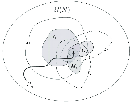
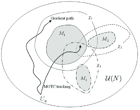
Fig. 1: Quantum Pareto optimal control aims to maximize the expectation values $\langle\Theta_{k}\rangle$, $k=1,\cdots,m~{}$ ($m=3$ in the present case). For each observable, the expectation value is maximized on a continuous submanifold $\mathcal{M}_{k}^{(\max)}$ of unitary propagators $U(T)$, the dimension of which is determined by the rank and eigenvalue degeneracies of the initial density matrix $\rho(0)$ and $\Theta_{k}$. The observables can be simultaneously maximized if the intersection $\bigcap_{k}\mathcal{M}_{k}^{(\max)}$ is nonempty and a point in the intersection can be reached under some time-dependent field $\varepsilon(t)$ (left panel). This intersection is a subset of the set of strongly Pareto optimal propagators $\mathcal{P}^{U}_{s}$, also called the Pareto frontier. Depending on $\rho(0)$ and $\{\Theta_{k}\}$, some problems may not have a completely optimal solution, and may involve a tradeoff between maximization of different observables. The set $\mathcal{P}^{U}_{w}$ of weakly Pareto optimal propagators consists of the union of intersections of the various $\mathcal{M}_{k}^{(\max)}$ with level sets $\{U(T)~{}|~{}\langle\Theta_{k}(T)\rangle=\chi_{k}\}$ of other observables (right panel). Optimization of multiobjective scalar cost functionals on the domain $\varepsilon(\cdot)$ (for example through gradient flows) does not generally lead to Pareto optima. Pareto optimal tracking control involves computational identification of points in $\mathcal{P}^{U}_{s}$ or $\mathcal{P}^{U}_{w}$ and subsequent experimental tracking of a direct path to that manifold on $\varepsilon(\cdot)$.

in many cases the $\Phi_{k}$ cannot be simultaneously maximized. Thus, the scalar concept of optimality must be replaced by the notion of Pareto optimality Statnikov and Matusov (1990). A control field $\varepsilon^{*}(t)$ is said to be strongly Pareto optimal if all other fields $\varepsilon(t)$ have a lower value for at least one of the objective functions $\Phi_{k}(\cdot)$, or else have the same value for all objectives. $\varepsilon^{*}(t)$ is weakly Pareto optimal if there does not exist another field $\varepsilon(t)$ such that $\Phi_{k}(\varepsilon(t))>\Phi_{k}(\varepsilon^{*}(t))$ for all $k$. Analogous definitions hold for strongly and weakly Pareto optimal unitary propagators $U^{*}(T)$, which we refer to as kinematic Pareto optima in order to distinguish them from the aforementioned dynamic Pareto optima. Fig. 1 provides examples of strong and weak kinematic Pareto optima. We denote the set of strong (kinematic, dynamic) Pareto optima by $\mathcal{P}^{(U,\varepsilon)}_{s}$, and the set of weak Pareto optima by $\mathcal{P}^{(U,\varepsilon)}_{w}$. We will use the term Pareto frontier (or Pareto front) to refer to $\mathcal{P}^{(U,\varepsilon)}_{s}$ or $\mathcal{P}^{(U,\varepsilon)}_{w}$. Our primary interest in this paper is the development of algorithms for sampling weak Pareto optima, which are much more numerous in quantum control problems than are strong Pareto optima. Note that it is possible to define the notion of Pareto optimality for more general cost functions; in particular, selected observable expectation values may be minimized through the replacements $\Phi_{k}(\cdot)\rightarrow-\Phi_{k}(\cdot)$.

A natural scalar objective function $\Phi$ for multiobservable control is a positively weighted convex sum of the individual observable objectives, i.e.,

$$\Phi_{M}(U)=\sum_{k=1}^{m}\alpha_{k}\Phi_{k}(U),\quad\alpha_{k}>0,$$ (3)

where $\Phi_{k}={\rm Tr}(U(T)\rho(0)U^{{\dagger}}(T)\Theta_{k}),\quad k=1,2,\cdots,m$. Within the electric dipole formulation, where the Hamiltonian assumes the form

$$H(t)=H_{0}-\mu\cdot\varepsilon(t)$$ (4)

with internal Hamiltonian $H_{0}$ and electric dipole operator $\mu$, the gradient of $\Phi_{M}$ is Ho and Rabitz (2006):

$$\frac{\delta\Phi_{M}}{\delta\varepsilon(t)}=-\frac{\imath}{\hbar}\sum_{k}\alpha_{k}{\rm Tr}\{\left[\Theta_{k}(T),\mu(t)\right]\rho(0)\},$$ (5)

where $\mu(t)=U^{{\dagger}}(t)\mu U(t)$. One approach to quantum Pareto optimal control is to employ gradient flow algorithms of the form

$$\frac{\partial\varepsilon_{s}(t)}{\partial s}=\gamma\frac{\delta\Phi_{M}}{\delta\varepsilon_{s}(t)},$$ (6)

where $\gamma$ is an arbitrary positive constant and $s$ is a continuous variable parameterizing the algorithmic search trajectory, to maximize an objective function or the form (3). In order to sample the Pareto front, various settings of the convex weights in (3) are typically sampled in independent optimizations Lin (1976). Note that the objective function $\Phi_{M}$ is just the expectation value of a single quantum observable $\Theta_{M}=\sum_{k=1}^{m}\alpha_{k}\Theta_{k}$. The absence of local traps Chakrabarti and Rabitz (2007) in control landscapes for the single observable objective function (2) thus indicates that the multiobservable gradient flow will also reach its global optimum . However, it is not immediately clear whether the multiobservable gradient flow (6) converges to points on the Pareto front, since the global optima of (2) for $\Theta=\Theta_{k}$ and (3) do not necessarily intersect. The same question arises for stochastic optimization of (3). We now examine the conditions under which (6) will converge to a weak Pareto optimum.

III Identification of Pareto optima

In order to understand the structure of the set $\mathcal{P}^{U}_{w}$ of weakly Pareto optimal points, it is necessary to first characterize the global optima of the individual objectives. The condition for a unitary propagator $U$ to be a critical point of objective function (2) is Wu et al. (2008):

$$[\Theta_{k},U\rho(0)U^{{\dagger}}]=0.$$ (7)

Let $\rho(0)$ and $\Theta_{k}$ be diagonalized according to $\tilde{\rho}=R^{{\dagger}}\rho(0)R$, $\tilde{\Theta}_{k}=S_{k}^{{\dagger}}\Theta_{k}S_{k}$, such that

$$\tilde{\rho} = diag\{\lambda_{(1)},\cdots,\lambda_{(1)};\cdots;\lambda_{(r)},\cdots,\lambda_{(r)}\}$$ (8)

$$\tilde{\Theta}_{k} = diag\{\gamma_{k(1)},\cdots,\gamma_{k(1)};\cdots;\gamma_{k(s_{k})},\cdots,\gamma_{k(s_{k})}\},$$ (9)

where the $\lambda_{(i)},~{}\gamma_{k(i)}$ are distinct eigenvalues of $\rho(0),\Theta_{k}$ with multiplicities $n_{1},\cdots,n_{r}$ and $m_{k1},\cdots,m_{ks_{k}}$, respectively. Further, set $\tilde{U}\equiv R^{{\dagger}}US_{k}$. We choose $R$ such that $\lambda_{(1)}<\cdots<\lambda_{(r)}$ and $S_{k}$ such that $\gamma_{k(1)}<\cdots<\gamma_{k(s_{k})}$. A diagonal matrix of eigenvalues satisfying this condition is said to be “arranged in increasing order”.

It was shown in Wu et al. (2008) that the critical submanifolds $\mathcal{M}_{k}^{i}$ that satisfy equation (7) for each objective $\Phi_{k}$ may be expressed in terms of $\tilde{U}$ as the double cosets

$$\mathcal{M}_{k}^{i}=\mathcal{U}(\textbf{n})\pi^{i}\mathcal{U}(\textbf{m}_{k}),$$ (10)

where $\mathcal{U}(\textbf{m}_{k})$ is the product group $\mathcal{U}(m_{k1})\times\cdots\times\mathcal{U}(m_{ks_{k}})$, each $\mathcal{U}(m_{kl})$ corresponding to an eigenvalue of $\Theta_{k}$ with $m_{kl}$-fold degeneracy (respectively $\mathcal{U}(\textbf{n}),\mathcal{U}(n_{1})\times\cdots\times\mathcal{U}(n_{r}),~{}\rho(0)$,$~{}n_{l}$), and $\pi^{i}$ denotes a permutation matrix on $N$ indices. We denote by $diag\{\gamma_{k1}^{\pi},\cdots,\gamma_{kN}^{\pi}\}=\pi^{{\dagger}}\tilde{\Theta}_{k}\pi$ the diagonal matrix of (possibly degenerate) eigenvalues resulting from application of a permutation $\pi$ to $\tilde{\Theta}_{k}$.

If two permutation matrices $\pi^{1},\pi^{2}$ satisfy the relation

$$\pi^{2}=U\pi^{1}V,\quad(U,V)\in\mathcal{U}(\mathbf{n})\times\mathcal{U}(\mathbf{m}_{k}),$$ (11)

then they are associated with the same critical submanifold, and we write $\pi^{1}\sim\pi^{2}$. By this equivalence relation, we can partition the permutation group $\mathcal{D}(N)$ into nonintersecting subsets:

$$\mathcal{P}(N)=\mathcal{D}_{k}^{1}\cup\cdots\cup\mathcal{D}_{k}^{d_{k}},$$ (12)

where each subset is an equivalence class with respect to $\sim$ and uniquely corresponds to a critical submanifold; $d_{k}$ is the number of critical submanifolds. For simplicity, we always let $\mathcal{D}_{k}^{\max}=\mathcal{D}_{k}^{1}$ correspond to the optimum manifold $\mathcal{M}_{k}^{\max}$, whose elements arrange the eigenvalues of $\tilde{\Theta}_{k}$ in increasing order.

Analytical results concerning the distribution of Pareto optima are most readily derived in the case where the observables $\{\Theta_{k}\}$ commute. In this case, they can be simultaneously diagonalized by a single unitary transformation $S$. Because the partition (12) for each $k$ is complete, each $\mathcal{D}_{k}^{i}$ must overlap with at least one $\mathcal{D}_{k^{\prime}}^{j}$. Hence, the critical manifolds $\bigcup_{i}\mathcal{M}_{k}^{i}$ and $\bigcup_{j}\mathcal{M}_{k^{\prime}}^{j}$ of $\Phi_{k}$ and $\Phi_{k^{\prime}}$, respectively, must intersect. The critical submanifolds $\mathcal{M}_{k}^{i}$ and $\mathcal{M}_{k^{\prime}}^{j}$ intersect if the corresponding $\mathcal{D}_{k}^{i}\cap\mathcal{D}_{k^{\prime}}^{j}\neq\emptyset$.

Based on the above result, we can specify the relationship between the maximum of the function $\Phi_{M}(U)$ and the critical submanifolds of the single observable cost functions $\Phi_{k}(U)$ in the case that the $\{\Theta_{k}\}$ commute. Let $\Theta_{M}\equiv\sum_{k=1}^{m}\alpha_{k}\Theta_{k}$, let $\mathcal{P}(N)=\mathcal{D}_{M}^{1}\cup\cdots\cup\mathcal{D}_{M}^{d_{M}}$ be the corresponding partition of permutation group, and let $S$ denote the unitary transformation that arranges $\tilde{\Theta}_{M}$ in increasing order. Then we have the following lemma pertaining to the conditions for convergence of gradient flow (6) to a Pareto optimum.

Lemma 1

Let $\{\Theta_{k}\}$ be a set of mutually commuting observables. The gradient flow (6) may (depending on initial conditions) converge arbitrarily close to a weak Pareto optimum if for at least one $k$, $\mathcal{D}_{k}^{\max}\cap\mathcal{D}_{M}^{\max}\neq\emptyset$. The flow is guaranteed to converge to a weak Pareto optimum if for each $~{}\mathcal{U}(m_{Mi})$ we have $S_{k}^{{\dagger}}S~{}\mathcal{U}(m_{Mi})~{}S^{{\dagger}}S_{k}\subseteq\mathcal{U}(m_{kj})$ for some $j$, and $\mathcal{D}_{M}^{\max}\subseteq\mathcal{D}_{k}^{\max}$. The flow may converge arbitrarily close to a strong Pareto optimum if $\mathcal{D}_{k}^{\max}\cap\mathcal{D}_{M}^{\max}\neq\emptyset$ for all $k$. For each $\Theta_{k}$, the flow may converge arbitrarily close to the critical submanifold $\mathcal{M}_{k}^{i}$ of $\Phi_{k}$ if $\mathcal{D}_{k}^{i}\cap\mathcal{D}_{M}^{\max}\neq\emptyset$.

The proof for guaranteed convergence to $\mathcal{P}_{w}^{(U,\varepsilon)}$ is presented in Appendix A. The remaining claims follow directly from the arguments above.

Now consider the problem of solving for the coefficients $\{\alpha_{k}\}$ such that the gradient flow is capable of converging to an arbitrarily specified combination of $l\leq m$ critical submanifolds of the respective observable operators, i.e.,

$$\Phi_{k}(U)=\chi_{k}^{i_{k}},\quad\chi_{k}^{i_{k}}\in\mathcal{C}_{k},\quad 1\leq k\leq l,$$ (13)

where $\chi_{k}^{i_{k}}$ denotes the $i_{k}$-th critical value in the set $\mathcal{C}_{k}$ of critical values of $\Phi_{k}(U)$. Let us write $\tilde{\Theta}_{M}=S^{{\dagger}}\Theta_{M}S=diag\{\sum_{k}\alpha_{k}\gamma_{k1}^{\pi_{k}},\cdots,\sum_{k}\alpha_{k}\gamma_{kN}^{\pi_{k}}\}$, where $\pi_{k}$ is the permutation matrix that reorders the diagonal elements of $\tilde{\Theta}_{k}=S_{k}^{{\dagger}}\Theta_{k}S_{k}$ so that they are arranged in the order induced by $S$, i.e., $S=\pi_{k}^{{\dagger}}S_{k}\pi_{k}$. Provided that we have

$$\mathcal{D}_{1}^{i_{1}}\cap\cdots\cap\mathcal{D}_{l}^{i_{l}}\neq\emptyset,$$ (14)

then for each permutation matrix $\pi\in\mathcal{D}_{1}^{i_{1}}\cap\cdots\cap\mathcal{D}_{l}^{i_{l}}$, there is an independent system of $N!-1$ inequalities:

$$\sum_{j=1}^{N}\sum_{k=1}^{m}\alpha_{k}\lambda_{j}\left(\gamma_{kj}^{\pi}-\gamma_{kj}^{\pi^{\prime}}\right)\geq 0,~{}~{}\forall\pi^{\prime}\neq\pi.$$ (15)

It is possible to satisfy conditions (13) at the global optimum of the objective function (3) if a solution to this set of inequalities exists for at least one such $\pi$. We therefore have the following theorem.

Theorem 1

Consider a quantum Pareto optimization problem of the form (13) involving mutually commuting observables $\{\Theta_{k}\}$.

1. It is possible to design an objective function (3) whose gradient flow may (depending on initial conditions) converge arbitrarily close to a weak Pareto optimum corresponding to $\chi_{k}^{i_{k}}=\chi_{k}^{\max}$ while arranging the expectation values of observables $\Theta_{k^{\prime}},~{}k^{\prime}\neq k$ in the order designated by equation (13), if a solution to the inequalities (15) exists for at least one $\pi\in\mathcal{D}_{1}^{i_{1}}\cap\cdots\cap\mathcal{D}_{l}^{i_{l}}.$

2. Similarly, it is possible to minimize the expectation value of observable $\Theta_{k}$ if a solution exists for $\chi_{k}^{i_{k}}=\chi_{k}^{\min}$.

3. If a solution exists for the choice $\{\chi_{k}^{i_{k}}\}=\{\chi_{k}^{\max}\}$, then it is possible to design an objective function (3) whose gradient flow converges arbitrarily close to a strong Pareto optimum.

The results of Theorem 1 pertaining to convergence to Pareto optima hold also for stochastic search algorithms that optimize a conventional multiobjective cost function of the form (3).

The relative likelihoods of the gradient flow (6) converging to various Pareto optima can be qualitatively assessed by comparing the dimension of $\mathcal{M}_{M}^{\max}$ to the dimension of the intersection $\mathcal{I}_{M,k}^{\max,\max}=\mathcal{M}_{M}^{\max}\cap\mathcal{M}_{k}^{\max}$ for each observable $k$ whose $\chi_{k}^{i_{k}}=\chi_{k}^{\max}$ in equation (13). These dimensions can be bounded analytically, according to a method described in Appendix A.

In the case that the $\{\Theta_{k}\}$ do not commute, the critical submanifold $\mathcal{M}_{k}^{i}$ of observable $\Theta_{k}$ does not necessarily intersect submanifold $\mathcal{M}_{k^{\prime}}^{j}$ of an observable $\Theta_{k^{\prime}}$ that is diagonal in a different basis even if $\mathcal{D}_{k}^{i}\cap\mathcal{D}_{k^{\prime}}^{j}\neq\emptyset$. In this case, a simple analytical criterion analogous to Lemma 1 for assessing whether (6) converges to a Pareto optimum does not exist, but a method presented in Appendix A may be used to determine the maximum possible dimension of the intersection sets.

The most common technique for sampling the Pareto front of multiobjective control problems is to run many independent maximizations of a cost functional like (3) on the domain $\varepsilon(t)$, using different coefficients $\{\alpha_{k}\}$. The results of Lemma 1 and Theorem 1 indicate conditions under which this strategy may be successful in quantum Pareto optimal control, and demonstrate that it may not always constitute a viable method. Even when the global optimum of a multiobjective cost function intersects the Pareto front, it is not necessarily advisable to employ such a function for Pareto front sampling on $\varepsilon(t)$, due to the considerable expense of each optimization on this high-dimensional domain Chakrabarti et al. (2008).

An alternative, generic approach to accelerating Pareto front sampling is to employ stochastic search algorithms that do not rely on optimization of a scalar objective function. In recent years, several such multiobjective genetic or evolutionary algorithms (MOEAs) - including the elitist nondominated sorted genetic algorithm (NSGA-II) Deb et al. (2002), the Pareto-archived evolution strategy (PAES) Knowles and Corne (1999) and strength-Pareto evolutionary algorithm (SPEA) Zitzer and Thiele (1999) - have been designed for the problem of multiobjective Pareto front sampling. These algorithms successively sort populations based on nondominance. The NSGA-II algorithm was applied successfully to the two-objective problem of optimal quantum dynamical discrimination Bonacina et al. (2007). While promising, MOEAs share several drawbacks, most notably a computational complexity that scales as $\mathcal{O}(md^{2})$ or $\mathcal{O}(md^{3})$, where $d$ denotes the population size. For problems involving control of a large number of observables, these algorithms - in addition to being less precise than deterministic algorithms - become very expensive since large population sizes are required to adequately sample the front.

Due to the fact that the quantum control cost functionals (2) are explicit functions of the final unitary propagator $U(T)$, but only implicit functions of the control field $\varepsilon(t)$, there exists a convenient alternative to either of the above Pareto optimization strategies based on a hybrid approach that combines kinematic and dynamic sampling. Assuming full controllability Ramakrishna et al. (1995), there is at least one $\varepsilon(t)$ in $\mathcal{P}_{w}^{\varepsilon}$ that maps to any given $U(T)$ in $\mathcal{P}_{w}^{U}$. The distribution of $\mathcal{P}_{w}^{U}$ in the domain $\mathcal{U}(N)$ is determined solely by the properties of $\rho(0)$ and the $\{\Theta_{k}\}$. Therefore, provided that the initial density matrix $\rho(0)$ is known, it is possible to sample Pareto optima on $\mathcal{U}(N)$; this sampling on a finite-dimensional space will be much more efficient than direct sampling of $\mathcal{P}_{w}^{\varepsilon}$. Once target points in $\mathcal{P}_{w}^{U}$ have been numerically identified, one may experimentally track a direct path to the corresponding points in $\mathcal{P}_{w}^{\varepsilon}$, using techniques that will be described in Section IV.

For example, many different coefficient sets $\{\alpha_{k}\}$ may be rapidly sampled using the kinematic gradient flow Chakrabarti et al. (2008) of the multiobservable objective function (3), namely

$$\frac{{\rm d}U}{{\rm d}s}=\sum_{k=1}^{m}\alpha_{k}[\Theta_{k},U\rho(0)U^{{\dagger}}]U,$$ (16)

instead of the dynamic flow (6). In the case that this flow converges to a (weak) Pareto optimum, it is a very convenient means of sampling segments of the front due to its speed. Of course, single observable kinematic gradient flows may always be used to locate a weakly Pareto optimal point, but do not provide the freedom to preferentially weight the importance of the other observables. Dividing the $m$ observables into mutually commuting sets and applying the weighted flow (16) for each set, with the $\{\alpha_{k}\}$ determined by solving the system of inequalities (15), provides a simple and rapid means of sampling the (weak) Pareto optima associated with a specified combination (13) of multiple expectation value constraints.

In the more general case where the $\{\Theta_{k}\}$ cannot be conveniently subdivided into mutually commuting subsets, the analytical results above on the distribution of Pareto optima are not immediately useful, but it is straightforward to determine numerically whether certain types of weak and strong Pareto optima exist. Given an estimate for $\rho(0)$, and the expectation values of $m$ observables at time $T$ specified as the control targets, the submanifold of unitary propagators $U(T)$ within which the actual propagator may lie is defined by the system of equations

$${\rm Tr}(U(T)\rho(0)U^{{\dagger}}(T)\Theta_{k}) = \chi_{k},\quad k=1,...,m,$$ (17)

$$\left[U^{{\dagger}}(T)U(T)\right]_{ij} = \delta_{ij},\quad i,j=1,...,N,$$ (18)

where $\chi_{k}$ is the desired expectation value of $\Theta_{k}$. If $\rho(0)$ is full-rank and nondegenerate, the rank of this system of equations in the $2N^{2}$ real variables $\mathrm{Re}\left(U_{ij}\right),\mathrm{Im}\left(U_{ij}\right)$ is maximal, resulting in the smallest possible dimension of the solution submanifold in $\mathcal{U}(N)$. Note that this system of equations is overdetermined if

$$m>2Nn-n^{2},\quad n={\rm rank}~{}\rho(0),$$ (19)

provided $\{\Theta_{k}\}$ is linearly independent. For example, if $\rho(0)$ is a pure state, parameterized by $N$ complex coefficients subject to a normalization constraint, then no more than $2N-1$ independent observables can be simultaneously driven to arbitrary expectation values. Multiobservable controllability amounts to controllability over a subset of the independent parameters of $\rho(0)$.

It is convenient to apply the principle of entropy maximization (PEM) in choosing a target $W$ from the solution submanifold, since this identifies a propagator that is most likely, from the perspective of statistical uncertainty, to be the real propagator of the system given the measurements made during multiobservable control. In this approach Buzek et al. (1999), the von Neumann entropy

$$S(\rho)={\rm Tr}(\rho\log\rho),~{}~{}~{}~{}\rho(U(T))=U(T)\rho(0)U^{{\dagger}}(T),$$ (20)

is maximized on $\mathcal{U}(N)$ subject to the constraints (17).

The following protocol then constitutes a general strategy for kinematic sampling of Pareto optima: 1) determine the maximum and minimum expectation values of each of the individual observables (by simple matching of the eigenvalues of $\rho(0)$, $\Theta_{k}$); 2) choose putative sets of observable expectation values $\{\chi_{k}\}$ within these respective ranges (setting $l<m$, $l=m$ of these expectation values to $\chi_{k}^{\max}$ for weak Pareto optima, strong Pareto optima respectively); 3) maximize the von Neumann entropy (using, for example, the simplex or Newton-Raphson algorithms with the constraints imposed as Lagrange multipliers), assuming the system of equations (17) above is consistent.

In the next section, we describe experimentally implementable algorithms for the optimization of multiple observable expectation values on the domain of controls $\varepsilon(t)$, which can be used in conjunction with the above kinematic algorithms to efficiently sample the dynamic Pareto front.

IV Pareto optimal tracking control

Once the target observable expectation values $\chi_{k},~{}k=1,\cdots,m$ on the Pareto front have been determined, it is possible to identify corresponding Pareto optimal control fields $\varepsilon^{*}(t)$ through minimization of an objective function of the following form:

$$\Phi_{M}^{\prime}(U)=\sum_{k=1}^{m}\alpha_{k}|\Phi_{k}(U)-\chi_{k}|^{2},\quad\alpha_{k}>0$$ (21)

over $\varepsilon(t)$, instead of maximization of (3). However, as described in Chakrabarti et al. (2008), gradient flow algorithms of this type can be inefficient, especially when the rank of the initial density matrix $\rho(0)$ is high, as it may be in large molecular systems or at elevated temperatures. Moreover, it is inconvenient to employ optimization of (21) to systematically investigate families of fields $\varepsilon^{*}(t)$ that differ in other experimentally relevant dynamic properties. In this section, we review and extend the more versatile methodology of multiobservable tracking control (MOTC), which drives the expectation values of $m$ observable operators along predetermined paths to the target $\{\chi_{k}\}$ Chakrabarti et al. (2008). Once an $\varepsilon^{*}(t)$ has been found, MOTC can be used to continuously trace the dynamic front to identify solutions that minimize the expenditure of control resources.

We assume, without loss of generality, that the observables $\Theta_{1},...,\Theta_{m}$ measured at each step of the search are linearly independent. Let $\Phi_{s}^{1},\cdots,\Phi_{s}^{m}$ denote the expectation value paths (functions of an algorithmic parameter $s$) for each observable, which together constitute a desired path $\textbf{w}_{s}$ of $\vec{\Phi}$ in the vector space of multiobservable expectation values. Then, the change in the control field along the track $\frac{\partial\varepsilon_{s}(t)}{\partial s}$ must satisfy the following condition:

$$\frac{{\rm d}\Phi_{s}^{i}}{{\rm d}s}=\int_{0}^{T}\frac{\delta\Phi_{s}^{i}}{\delta\varepsilon_{s}(t)}\frac{\partial{\varepsilon_{s}(t)}}{\partial s}{\rm d}t=\frac{{\rm d}\textbf{w}_{s}^{i}}{{\rm d}s}.$$ (22)

where $\Phi_{i}={\rm Tr}(U(T)\rho(0)U^{\dagger}(T)\Theta_{i})$ This is a Fredholm integral eqn of the first kind for the unknown partial derivative $\frac{\partial{\varepsilon_{s}(t)}}{\partial s}$, given $\varepsilon_{s}(t)$ at $s$ and all $t\in[0,T]$. To solve for the algorithmic flow $\frac{\partial\varepsilon_{s}(t)}{\partial s}$ that tracks $\textbf{w}_{s}$, it is necessary to expand it on a basis of independent functions. It is convenient to make this expansion on the basis of the independent observable expectation value gradients:

$$\frac{\partial\varepsilon_{s}(t)}{\partial s}=\sum_{j=1}^{m}x^{j}_{s}\frac{\delta\Phi_{s}^{j}}{\delta\varepsilon_{s}(t)}+f_{s}(t),$$ (23)

where $f_{s}(t)$ contains the degrees of freedom outside the subspace spanned by $\frac{\delta\Phi_{s}^{j}}{\delta\varepsilon_{s}(t)}$. As described in Chakrabarti et al. (2008), $f_{s}(t)$ can take on a variety of forms depending on auxiliary dynamical costs on $\varepsilon(t)$ that are to be minimized. Inserting the expansion (23) into the integral equation (22), we have

$$\sum_{j=1}^{m}x^{j}_{s}\int_{0}^{T}\frac{\delta\Phi_{s}^{i}}{\delta\varepsilon_{s}(t)}~{}\frac{\delta\Phi_{s}^{j}}{\delta\varepsilon_{s}(t)}{\rm d}t=\frac{{\rm d}\textbf{w}^{i}_{s}}{{\rm d}s}-\int_{0}^{T}\frac{\delta\Phi_{s}^{i}}{\delta\varepsilon_{s}(t)}f_{s}(t){\rm d}t.$$

Defining the $m$-dimensional vector $\textbf{a}_{s}(t)=(a_{s}^{1}(t),\cdots,a_{s}^{m}(t))$ by

$$a_{s}^{i}(t)=\frac{\delta\Phi_{s}^{i}}{\delta\varepsilon_{s}(t)}=-\frac{\imath}{\hbar}{\rm Tr}\left(\rho(0)\big{[}U^{{\dagger}}_{s}(T)\Theta_{i}U_{s}(T),\mu_{s}(t)\big{]}\right),$$

and the MOTC Gramian matrix $\Gamma_{s}$ by

$$(\Gamma_{s})_{ij}=\int_{0}^{T}a^{i}_{s}(t^{\prime})a^{j}_{s}(t^{\prime}){\rm d}t^{\prime},$$ (24)

it can then be shown Chakrabarti et al. (2008) that the initial value problem for $\varepsilon_{s}(t)$ given $\varepsilon_{0}(t)$ is:

$$\frac{\partial\varepsilon_{s}(t)}{\partial s}=f_{s}(t)+\left[\frac{{\rm d}\textbf{w}}{{\rm d}s}-\int_{0}^{T}\textbf{a}_{s}(t^{\prime})f_{s}(t^{\prime}){\rm d}t^{\prime}\right]^{T}\Gamma_{s}^{-1}\textbf{a}_{s}(t).$$ (25)

This expression can be integrated either numerically (using standard methods described in Chakrabarti et al. (2008)) or experimentally (Section V) to track the desired path $\textbf{w}_{s}$ to the dynamic Pareto front. The invertibility of the Gramian matrix $\Gamma_{s}$ corresponds to the ability to move from the point $\vec{\Phi}_{s}$ in multiobservable space to any infinitesimally close point $\vec{\Phi}_{s+{\rm d}s}$ through an infinitesimal change $\delta\varepsilon_{s}(t)$ in the control field Chakrabarti et al. (2008). With minor modifications Chakrabarti et al. (2008), the MOTC tracking differential equation (25) can also be used to carry out multiobjective optimizations for non-observable objectives.

The MOTC algorithm can be applied to follow any arbitrary vector track $\textbf{w}_{s}$ of observable expectation values. It is convenient to choose $\textbf{w}_{s}$ based on the corresponding set of possible paths $U_{s}(T)$ in the domain $\mathcal{U}(N)$ of unitary propagators, since the latter contains the most information about the dynamics of the system at time $T$. Let $\mathcal{L}_{s}=\{V_{s}~{}|~{}\Phi_{k}(V_{s})=w_{s}^{k},~{}k=1,...,m\}$ denote the set of propagators that map to the observable track at algorithmic time $s$. Denote by $B_{s}$ the system of equations (17) with $\{\chi_{k}\}$ replaced by $\textbf{w}_{s}$. Assuming this system is consistent, the dimension of $\mathcal{L}_{s}$ is equal to $N^{2}$ less the number of independent equations in $B_{s}$. As such, the path $U_{s}(T)$ followed by the optimization algorithm in $\mathcal{U}(N)$ will, on average, be more similar to a target unitary track $Q_{s}$, for a greater number $m$ of orthogonal observables (note $\mathrm{dim}~{}\mathcal{L}_{s}$ also depends on the eigenvalue spectra of $\rho(0)$ and $\{\Theta_{k}\}$). As a function of the algorithmic step $s$, the term $\left[\int_{0}^{T}\textbf{a}_{s}(t^{\prime})f_{s}(t^{\prime}){\rm d}t^{\prime}\right]^{T}\Gamma_{s}^{-1}$ in equation (25) will adjust the step direction so that the possible unitary propagators $V_{s}$ at each step are constrained within the subspace $\mathcal{L}_{s}$ (provided $\Gamma$ is invertible; see Section VI). In Section V, we describe special choices for $\textbf{w}_{s}$ that are globally optimal from the standpoint of mean distance traveled in $\mathcal{U}(N)$.

An alternative MOTC-based approach to identifying weak dynamic Pareto optima is to maximize the expectation values of successive observable operators while holding those previously maximized at constant values. This requires successively applying $m$ MOTC searches of dimensions $1,\cdots,m$, respectively; these searches may be carried out in an order that reflects the relative importance of the observable objectives. Let $(p_{1},\cdots,p_{m})$, where $p$ is a permutation on $m$ indices, denote this order and let $\chi^{p_{i}}$ denote the conditional maximum of $\Phi^{p_{i}}(\varepsilon(t))$ given $\Phi^{p_{j}}(\varepsilon(t))=\chi^{p_{j}},~{}1\leq j<i$. This approach then amounts to successive integrations of (25) with

$$\textbf{w}_{s}^{(r)} = (\chi^{p_{1}},\cdots,\chi^{p_{r-1}},w_{s}^{r}),$$ (26)

$$\textbf{a}_{s}^{(r)} = (a_{s}^{p_{1}},\cdots,a_{s}^{p_{r}}),\quad r=1,\cdots,m,$$ (27)

where $w_{s}^{r}$ is any monotonically increasing function of $s$. For maximization of $m$ observables, there are $m!$ such combinatorially distinct control strategies.

The final observable expectation values $\{\chi_{k}\}$ will seldom be the only properties of a control solution that are relevant experimentally. In general, other dynamic properties of the field, such as its total fluence $\int_{0}^{T}\varepsilon^{2}(t)dt$, will have implications for the feasibility of a control experiment. Hence, the ability to continuously traverse a submanifold of the dynamic Pareto front, once it has been found, may be essential for identifying a Pareto optimal control $\varepsilon^{*}(t)$ with the most desirable physical properties. There generally exists an infinite number of control field solutions corresponding to any given combination of final observable expectation values $\{\chi_{k}\}$, as evidenced by the presence of the free function $f_{s}(t)$ in equation (25). The MOTC algorithm offers a systematic means of exploring these families of solutions through specification of $f_{s}(t)$. To maintain the objective function values $\{\Phi_{k}\}$ at their target values $\{\chi_{k}\}$ while sampling fields corresponding to a free function $f_{s}(t)$, the following initial value problem for $\varepsilon_{s}(t)$ is solved:

$$\frac{\partial\varepsilon_{s}(t)}{\partial s}=f_{s}(t)-\left[\int_{0}^{T}\textbf{a}_{s}(t^{\prime})f_{s}(t^{\prime}){\rm d}t^{\prime}\right]^{T}\Gamma_{s}^{-1}\textbf{a}_{s}(t).$$ (28)

With the observable expectation values fixed, different choices of the free function $f_{s}(t)$ correspond to different trajectories through the associated portion of the dynamic Pareto front. The final unitary propagator $U(T)$ may change during such excursions. Choosing $f_{s}(t)=-\frac{1}{\eta}\frac{\varepsilon_{s}(t)}{S(t)}$ , where $S(t)>0$ is an arbitrary weight function (e.g., a Gaussian) and $\eta$ is a constant that controls numerical instabilities, will minimize fluence at each algorithmic time step $s$ Rothman et al. (2006). Note that equation (28) can also be used to identify fluence-minimizing controls for other multiobservable control problems like optimal state preparation.

The connectedness of the submanifold of $\mathcal{P}_{w}^{\varepsilon}$ corresponding to the expectation values $\{\chi_{k}\}$ determines which $\varepsilon^{*}(t)$ can be accessed by application of (28). It has been shown Pechen et al. (2008) that the kinematic level sets $\{U(T)~{}|~{}\Phi_{k}(U(T))=\chi_{k}\}$ of single observables are connected manifolds. However, the dynamic level sets $\{\varepsilon(t)~{}|~{}\Phi_{k}(\varepsilon(t))=\chi_{k}\}$ may under certain circumstances Dominy and Rabitz (2008) be disconnected. Moreover, it is possible that the intersections of the kinematic level sets of multiple observables (i.e., the solutions to the system of equations (17)) consist of disconnected submanifolds. If this intersection is disconnected, it follows that the dynamical intersection set is also disconnected Dominy and Rabitz (2008).

A disadvantage of the purely dynamic Pareto front sampling strategy (26) is that since the manifold of control fields $\{\varepsilon(t)~{}|~{}\Phi_{k}(\varepsilon(t))=\chi_{k},~{}1\leq k\leq m\}$ to which the algorithm converges may in general consist of disconnected submanifolds, certain classes of solutions may not be accessible from a canonical starting field $\varepsilon^{*}(t)$ by the homotopy tracking algorithm (28). By contrast, sampling of the kinematic Pareto front by the methods described in Section III can (at the expense of additional initial overhead required for state estimation) identify propagators $U^{*}(T)$ that lie in different disconnected submanifolds of the front, such that (28) can subsequently be applied to reach any control field in the local vicinity of the canonical field $\varepsilon^{*}(t)$ obtained from application of (25). On the other hand, a virtue of the method (26) is that it is also applicable to quantum Pareto optimal control problems other than observable maximization, where kinematic identification of Pareto optima may not be possible.

Maximization of (21) or of (3) (assuming $\{\alpha_{k}\}$ are restricted to the ranges stipulated by the system of inequalities (15)), with various coefficient sets $\{\alpha_{k}\}$, will also lead to distinct points on the dynamic Pareto front with the same observable expectation values but different $U(T)$ and/or dynamic properties of the field. However, such a strategy is far less efficient than applying equation (28), since a separate optimization must be carried out for each set of coefficients. Further mathematical details on the formal correspondence between these two approaches, from the perspective of differential geometry, may be found in the treatise Hillermeier (2001).

The observables $\{\Theta_{k}\}$ of interest are not necessarily orthogonal. However, the statistical efficiency of MOTC (i.e., the tracking accuracy for a given number of measurements) is easiest to assess when orthogonal observables are measured at each step. For simplicity, we represent each of the Hermitian matrices as an $N^{2}$-dimensional vector with real coefficients. Then Gram-Schmidt orthogonalization offers a convenient means of constructing an orthogonal basis of $m$ linearly independent $N^{2}$-dimensional vectors, $\Theta^{\prime}_{1}(T),...,\Theta^{\prime}_{m}(T)$ that spans the associated subspace - any element of the set $\{\Theta_{k}\}$ can be expressed as a linear combination of the basis operators in this set, i.e., for any $k$, $\Theta_{k}=\sum_{i=1}^{m}c_{ki}\Theta^{\prime}_{i}$. When the desired tracks of the target observable expectation values are thus expanded on a set of experimentally measured orthogonal observables, we have

$$\frac{\delta\Phi_{k}}{\delta\varepsilon_{s}(t)}=-\frac{\imath}{\hbar}\sum_{i}c_{ki}{\rm Tr}\left(\left[\Theta_{i}^{\prime}(T),\rho(0)\right]\mu(t)\right)$$ (29)

for the gradient of each of the observable expectation values $\langle\Theta_{k}\rangle$ with respect to the control.

V Experimental implementation

This section discusses methodologies for the laboratory implementation of MOTC and Pareto optimal control. Laboratory implementation of quantum optimal control is typically carried out in open loop with numerical search algorithms guiding the experimental control field updates (e.g., via a laser pulse shaper) at each algorithmic step Levis et al. (2001).

V.1 Initial state estimation

In order to kinematically sample the Pareto front as described above, it is necessary to have an estimate for the initial density matrix $\rho(0)$. In the case that $\rho(0)$ is not a thermal mixed state, it can be determined by the method of maximal likelihood estimation (MLE) of quantum states Banaszek et al. (1999). Here, the likelihood function

$$L(\hat{\rho})=\prod_{i=1}^{n}{\rm Tr}(\hat{\rho}(0)\mathcal{F}_{i}),$$

where $\mathcal{F}_{i}$ denotes a positive operator valued measure (i.e., one of a complete set of $N^{2}-1$ orthonormal observable operators) corresponding to the outcome of the $i$-th measurement, describes the probability of obtaining the set of $n$ observed outcomes for a given trial density matrix $\hat{\rho}$. This likelihood function must be maximized over the set of admissible density matrices. An effective parameterization of $\hat{\rho}$ is the Cholesky decomposition $\hat{\rho}(0)=\hat{T}^{{\dagger}}\hat{T}$ – where $T$ is a complex lower triangular matrix with real elements along the diagonal – which guarantees positivity and Hermiticity. The remaining condition of unit trace is imposed via a Lagrange multiplier $\lambda$. Maximization of the function

$$\mathcal{L}(\hat{T})=\sum_{i=1}^{n}\ln{\rm Tr}(\hat{T}^{{\dagger}}\hat{T}\mathcal{F}_{i})-\lambda{\rm Tr}(\hat{T}^{{\dagger}}\hat{T}),$$

with the choice $\lambda=n$ for the Lagrange multiplier, guarantees normalization of $\hat{\rho}$ at the MLE estimate Banaszek et al. (1999). Standard numerical techniques, such as Newton-Raphson or uphill simplex algorithms, are used to search for the maximum of $\mathcal{L}$ over the $N^{2}$ parameters of the matrix $\hat{T}$.

V.2 Minimal-length $\textbf{w}_{s}$ and error correction

There are many possible choices for the track $\textbf{w}_{s}$ that leads to a point $W$ in $\mathcal{P}_{w}^{U}$. However, it is desirable to choose paths that are globally optimal from a geometric perspective. The Riemannian Bures metric on the space of density matrices Uhlmann (1976) could be used for this purpose, but this metric cannot be expressed in compact form for arbitrary Hilbert space dimensions, especially for arbitrary $m$-dimensional subspaces of the Hilbert space. We thus adopt the more convenient approach of defining the target multiobservable track as the $\textbf{w}_{s}$ that maps to the geodesic $Q_{s}$ in $\mathcal{U}(N)$ between any $U_{0}$ consistent with the initial control guess and $W$, i.e.,

$$\textbf{w}_{s}^{k}\equiv\sum_{i}c_{ki}{\rm Tr}\left\{\rho(0)Q_{s}^{{\dagger}}\Theta_{i}^{\prime}Q_{s}\right\},$$ (30)

where $Q_{s}=U_{0}\exp(\imath As)$ with $A=-\imath\log(W^{{\dagger}}U_{0})$.

Error-correction methods can be applied to account for deviations from the track $\textbf{w}_{s}$. These generally involve the addition of a correction term $\mathbf{c}_{s}$ to the tracking differential equation (25) such that

$$\frac{\partial\varepsilon_{s}(t)}{\partial s}=f_{s}(t)+\left[\mathbf{c}_{s}+\frac{{\rm d}\textbf{w}_{s}}{{\rm d}s}-\int_{0}^{T}\textbf{a}_{s}(t^{\prime})f_{s}(t^{\prime}){\rm d}t^{\prime}\right]^{T}\Gamma_{s}^{-1}\textbf{a}_{s}(t),$$ (31)

where $\mathbf{c}_{s}$ may be taken to be a scalar multiple of the difference between the actual vector of observable expectation values and the target track, i.e.,

$$\mathbf{c}_{s}=\beta(\mathbf{w}_{s}-\vec{\Phi}_{s}),~{}~{}~{}\beta>0.$$

Note that since this error-correction method requires only estimation of the expectation values of the $m$ observable operators $\{\Theta_{k}\}$, it is straightforward to implement in an experimental setting.

Runge-Kutta (RK) integration of the MOTC differential equation (31) can further decrease tracking errors by employing derivative information at multiple points across the algorithmic step, instead of only at a single point. In principle, RK may be applied experimentally at a substantially lower cost than including second order functional derivatives in the tracking differential equations, since the latter requires estimation of the Hessian matrix of the observable expectation values with respect to the control. Moreover, although it is possible to implement second-order MOTC numerically, accurate experimental estimation of the Hessian is difficult due to the inevitable presence of experimental noise. Thus, RK integration is the preferred method for further improvement of the experimental accuracy of MOTC algorithms.

V.3 Choice of measurement bases

Gram-Schmidt orthogonalization, as discussed in the previous section, is a convenient method for obtaining a canonical orthogonal observable basis for MOTC, but from the point of view of experimental overhead, it is generally not statistically efficient to measure these observables. The complete set of $N^{2}-1$ possible orthogonal observables can instead be expanded on $N+1$ orthonormal measurement bases. Here, we use mutually unbiased measurement bases (MUB) Wootters and Fields (1989), which are known to provide tight confidence intervals on the expectation values of a set of multiple observables for a finite number of measurements (the advantage in statistical efficiency increases with $m$). The expression for MUB differs based on the Hilbert space dimension $N$. When $N$ is the power of an odd prime (which encompasses all cases considered in the current work), these bases $V^{(r)}$ are given by

$$V_{pq}^{(r)}=\left\{\begin{array}[]{ll}\delta_{pq},&r=0\\ \\ \frac{1}{\sqrt{N}}\exp[\frac{2\pi i}{N}(rq^{2}+pq)],{}{}&1\leq r\leq N.\\ \end{array}\right.$$

The orthonormal observables $\Theta^{\prime}$ in equation (29) can then be taken to be

$$\Theta_{r(N-1)+i}^{\prime} = V^{(r)}\tilde{\Theta}_{i}^{\prime}(V^{(r)})^{{\dagger}},$$ (32)

$$\tilde{\Theta}_{i}^{\prime} = |i\rangle\langle i|=diag\{0,...,1,...0\},$$ (33)

for $1\leq i\leq N-1$, $0\leq r\leq N$. However, the orthonormal observables in these bases need not be projection operators.

Every quantum measurement in a basis $V^{(r)}$ provides information regarding the parameters $p_{1},...,p_{N}$ of the multinomial distribution corresponding to that basis ($N-1$ of these may be considered parameters of $\rho(T)$). The measurement of an observable $\Theta$ with $s$ distinct eigenvalues returns $s-1$ independent parameters from the set. Control of multiple observables can be achieved for the lowest experimental cost by measuring nondegenerate observables in the bases of interest. Moreover, tight bounds on those gradient estimates will be obtained if the measurement bases are mutually unbiased. Therefore, for each MUB basis, assume a full-rank, nondegenerate observable $\Theta$ is measured that is diagonal in that basis, i.e., $\Theta=V^{(r)}\Sigma(V^{(r)})^{{\dagger}},\quad\Sigma=diag\{\sigma_{1},\cdots,\sigma_{N}\}$. The multinomial distribution parameters $p_{1},...,p_{N-1}$ are then formally given by

$$p_{i}={\rm Tr}\left(\rho(T)V^{(r)}\tilde{\Theta}_{i}^{\prime}(V^{(r)})^{{\dagger}}\right),~{}1\leq i\leq N-1,$$

with the remaining $p_{N}=1-\sum_{i=1}^{N-1}p_{i}$. These correspond experimentally to the frequencies with which the measurement outcomes $\sigma_{i}$ are observed. Assuming for simplicity that the measurement basis $V^{(r)}$ has been chosen such that it coincides with a basis within which one of the $m$ target observables $\Theta_{k}$ is diagonal (extension to the more general case is straightforward), and writing $\Theta_{k}=V^{(r)}\Xi(V^{(r)})^{{\dagger}}$ where $\Xi=diag\{\gamma_{1},\cdots,\gamma_{N}\}$, the expectation values of the $m$ target observables at each MOTC step can then be written in terms of the experimentally estimated frequencies as

$$\langle\Theta_{k}\rangle=\sum_{i=1}^{N}c_{ki}p_{i}\gamma_{i},$$

where the $c_{ki}$ are the expansion coefficients in (29). This approach is generally more efficient than direct estimation of the $\langle\Theta_{k}\rangle$.

V.4 Gradient estimation

In an experimental setting, the gradients $\frac{\delta\Phi_{k}}{\delta\varepsilon_{s}(t)}$ may be estimated by statistical sampling of points near the current control field $\varepsilon_{s}(t)$ Roslund and Rabitz (2008) instead of the method of finite differences; the latter is inaccurate due to the inevitable presence of noise (e.g., laser noise) in the laboratory. Let us denote a discretized representation of the control field $\varepsilon(t)$ by the vector $\vec{x}$ (e.g., the 128 pixel settings in a laser pulse shaper) with associated domain $\mathcal{D}$, the point at which the gradient is evaluated by $\vec{x}_{0}$, and a symmetric distribution function around $\vec{x}_{0}$ over $\mathcal{D}$ by $\pi$.

It can be shown Roslund and Rabitz (2008) that the following expression constitutes a second-order approximation to $\nabla\Phi(\vec{x}_{0})$:

$$\nabla\Phi(\vec{x}_{0})\approx{\Sigma}^{-1}\int_{\mathcal{D}}(\vec{x}-\vec{x}_{0})\Phi(\vec{x})\pi(\vec{x}-\vec{x}_{0}){\rm d}\vec{x},$$

where the covariance matrix is

$${\Sigma}=\int_{\mathcal{D}}(\vec{x}-\vec{x}_{0})(\vec{x}-\vec{x}_{0})^{T}\pi(\vec{x}-\vec{x}_{0}){\rm d}\vec{x}.$$

This expression can be evaluated via Monte Carlo integration over $N_{\exp}$ measurement results:

$$\nabla\Phi(\vec{x}_{0})\approx\frac{{\Sigma}^{-1}}{N_{\exp}}\sum_{i=1}^{N_{\exp}}(\vec{x}^{(i)}-\vec{x}_{0})\Phi(\vec{x}^{(i)})\pi(\vec{x}^{(i)}-\vec{x}_{0}).$$

Open-loop steepest ascent control field search using a femtosecond laser pulse shaper, with the gradient evaluated at each iteration via this technique, successfully reached the global maximum of the control landscape for second harmonic generation Roslund and Rabitz (2008), indicating a robustness of such gradient-based search algorithms to noise.

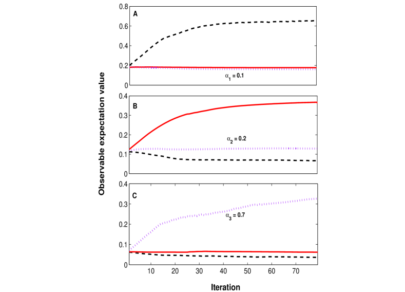
Fig. 2: MOTC-based Pareto optimum ($\mathcal{P}_{w}^{\varepsilon}$) sampling for three observables in an 11-level system. Weakly Pareto optimal unitary matrices were determined using the kinematic gradient (16) followed by MOTC to identify optimal controls. The convex weights in equation (3) were set to $\alpha_{1}=0.7,~{}\alpha_{2}=0.2,\alpha_{3}=0.1$ (dashed); $\alpha_{1}=0.2,~{}\alpha_{2}=0.7,\alpha_{3}=0.1$ (solid); $\alpha_{1}=0.1,~{}\alpha_{2}=0.2,\alpha_{3}=0.7$ (dotted). $\rho(0)$ was a thermal mixed state. A) Observable $\Theta_{1}$: rank three diagonal degenerate observable with the three highest energy levels targeted; B) Observable $\Theta_{2}=|2\rangle\langle 2|$; C) Observable $\Theta_{3}=|3\rangle\langle 3|$.

VI Examples

As a representative Pareto optimal control scenario, we apply tracking control to the weighted maximization of three mutually commuting observables. In addition, in order to illustrate the characteristic features of problems - such as optimal mixed state preparation - that require the control of $m>2N-1$ observables, we apply MOTC using multiple mutually unbiased measurement bases to a multiobservable control problem involving control of 40 observables in an 11-level system.

The tracking examples below employ an 11-dimensional Hamiltonian of the form (4), with

$$H_{0} = diag~{}\{0.1,0.2,\cdots,1.1\},$$ (34)

$$\mu_{ij} = \left\{\begin{array}[]{cl}1,&i=j;\\ 0.15,&|i-j|=1;\\ 0.08,&|i-j|=2;\\ 0,&\text{otherwise}.\end{array}\right.$$ (39)

It can verified (by checking that the rank of the Lie algebra generated by and $H_{0}$, $\mu$ equals $N^{2}$), that this system is fully (propagator) controllable Ramakrishna et al. (1995); Albertini and D’Alessandro (2003). MOTC and multiobservable gradient flow algorithms were implemented using the numerical methods described in Chakrabarti et al. (2008).

VI.1 Quantum control landscape Pareto front sampling

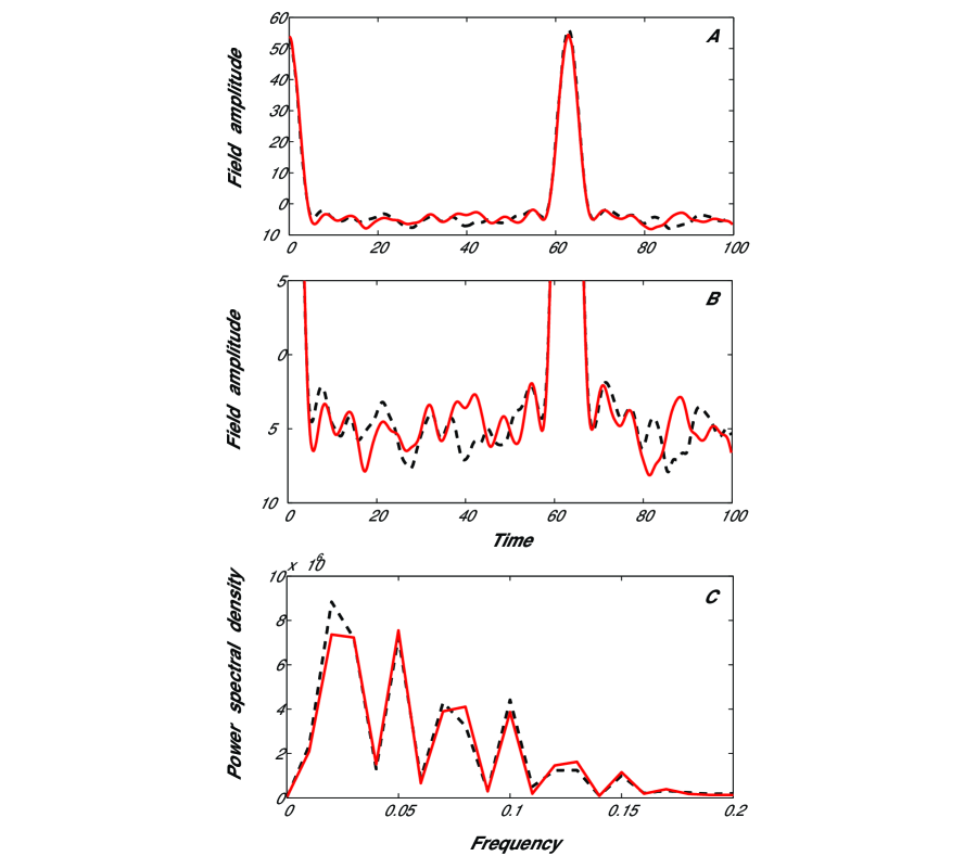
Fig. 3: Optimal control fields A), B) (magnified) and their Fourier power spectra C) obtained by the MOTC Pareto optimum sampling depicted in Fig. 2, for weights $\alpha_{1}=0.7,~{}\alpha_{2}=0.2,~{}\alpha_{3}=0.1$ (dashed) and $\alpha_{1}=0.2,~{}\alpha_{2}=0.7,~{}\alpha_{3}=0.1$ (solid). $\varepsilon_{0}(t)$ was of the form (40) with amplitudes weighted according to the number of times the frequency $\omega_{ij}$ appears in the transition frequency spectrum.

A common objective in quantum multiobservable maximization problems is the identification of control fields that maximize a single observable expectation value while selectively weighting the importance of increasing the expectation values of several auxiliary observables. As discussed above, such control fields are weakly Pareto optimal. These weak Pareto optima can be efficiently sampled using the methods described in Sections III and IV. As an example of weighted multiobservable maximization, several combinations of convex weights in multiobservable objective function (3) were employed in separate trials, representing desired trends in the relative magnitudes of the respective observable expectation values of three commuting observables; each observable was assigned the highest weight in several trials. The weakly Pareto optimal set corresponds in this case to points on $\varepsilon(t)$ where at least one of the 3 observable expectation values is at its maximum possible value; for the purposes of numerical illustration, $\sim 85\%$ of the maximum achievable value was considered sufficient. The kinematic gradient (16) was applied to maximize the multiobservable objective function on the domain $\mathcal{U}(N)$; in the case of these observables, it always reached a weakly Pareto optimal point. The expectation value of the observable assigned the highest weight reached the greatest value.

MOTC (equation (25)) was then applied to track multiobservable expectation value paths (30) to controls in $\mathcal{P}_{w}^{\varepsilon}$ that map to these points in $\mathcal{P}_{w}^{U}$ (Fig. 2). Fig. 3A compares the optimal control fields obtained by MOTC and their Fourier power spectra at a point on the weak Pareto optimum where observable 1 dominates, with those at a corresponding point where observable 2 dominates. These points do not lie on the same level set of any observable. Nonetheless, note that their Fourier power spectra (Fig. 3B) are very similar, indicating that many similar fields reside at the distinct weakly Pareto optimal manifolds corresponding to different dominant observables. By contrast, optimal fields that lie on the level set of a single observable may display very different Fourier spectra, if different numbers $m$ of observables are controlled (as shown in Fig. 6 below). This suggests that the major contributor to the complexity of optimal fields in Pareto optimal control problems is the number of parameters of the density matrix or $U(T)$ that are simultaneously constrained, and not the tradeoff between the expectation values of the various observables on the Pareto front.

In order to assess the advantage of precomputing a propagator in $\mathcal{P}_{w}^{U}$ and tracking to a corresponding point in $\mathcal{P}_{w}^{\varepsilon}$ via MOTC, the multiobservable dynamical gradient (5) was applied directly in an adaptive step size (line search) steepest ascent algorithm. Although the multiobservable gradient flow converged to a weak Pareto optimum, the dynamical gradient flow was substantially less efficient in most weighted multiobservable maximizations compared to single observable maximizations (data not shown). Typically, none of the $m$ observable expectation values increase monotonically in dynamical multiobservable steepest ascent, whereas the expectation value of the most highly weighted observable does rise monotonically in the kinematic multiobservable gradient flow, presumably due to the lower dimensionality of the search domain. In an experimental setting where noise may obscure minute differences in observable expectation values, application of steepest ascent may therefore not be as efficient as it has been found to be for the control of single observables Roslund and Rabitz (2008). By contrast, kinematic sampling on $\mathcal{U}(N)$ (after estimation of the state $\rho(0)$) is a reliable and rapid method of sampling $\mathcal{P}_{w}^{U}$.

In the above example, the observables were mutually commuting, i.e. belonged to the same measurement basis. In this case, the kinematic gradient flow (16) could be used to locate weakly Pareto dominant points, since the maximum submanifold $\mathcal{M}_{M}^{\max}$ of $\Phi_{M}$ intersected the maximum $\mathcal{M}_{k}^{\max}$ of one of the single observable cost functions $\Phi_{k}$ (here, the cost functions satisfied the conditions in Lemma 1 guaranteeing Pareto convergence). In the more general case where the targets are $m$-tuples of arbitrary observable expectation values, or points on the Pareto front where specific expectation values of the $m-1$ dominated observables are desired, the von Neumann entropy (20) can be maximized, instead of employing the kinematic gradient flow.

VI.2 Effect of state preparation

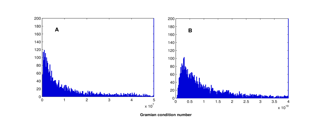
Fig. 4: Gramian matrix condition number distributions for an 11-level system (random internal Hamiltonian $H_{0}$ and dipole operator $\mu$): multiple measurement bases and the effect of state preparation. The amplitudes and phases of the modes of the control field $\varepsilon(t)$ were sampled randomly from the uniform distributions $(0,1]$ and $(0,2\pi]$, respectively, with the mode frequencies tuned to the transition frequencies of the system. A) MOTC, 20 observables: pure state $\rho(0)$. B) MOTC, 40 observables: pure state $\rho(0)$. Observables were drawn sequentially from successive mutually unbiased measurement bases in equation (32).

The MOTC Gramian matrix $\Gamma$ must be invertible at a given control field $\varepsilon_{s}(t)$ in order for the tracking algorithm to be able to follow any arbitrarily designated path to the Pareto front $\mathcal{P}_{w}^{\varepsilon}$. Typically, a Gramian condition number $C>10^{9}$ results in large numerical errors upon inversion, and would be expected to compromise the accuracy of tracking, due to the sparseness of control field increments $\delta\varepsilon(t)$ that are capable of driving the system to the arbitrary neighboring states.

As the number of controlled observables $m$ increases, the condition number $C$ can rise steeply beyond a critical $m$, where additional observables cannot be assigned arbitrary local tracks. Analytically, when the condition (19) is satisfied, the $m$ functions of time $\frac{\delta\Phi_{k}}{\delta\varepsilon(t)}$ that dictate local multiobservable controllability cannot remain linearly independent, resulting in an ill-conditioned Gramian $\Gamma$. This feature of multiobservable local controllability is independent of the Hamiltonian. However, in practice, condition numbers typically do not explode at a critical $m$, due to numerical inaccuracies in the singular value decomposition of matrices that are close to singular.

Fig. 4 compares the $\Gamma$ condition number distributions for a system with pure $\rho(0)$, for $m_{1}=20$ and $m_{2}=40$, using randomly sampled fields $\varepsilon(t)$ of the form

$$\varepsilon(t)=\sum_{i=1}^{N}\sum_{j=i+1}^{N}A_{ij}\sin\left(\omega_{ij}t+\phi_{ij}\right),\quad 0\leq t\leq T,$$ (40)

where $\omega_{ij}=|E_{i}-E_{j}|$ denote the transition frequencies between energy levels $E_{i},~{}E_{j}$ of $H_{0}$, $\phi_{ij}$ denotes a phase sampled uniformly within the range $(0,2\pi]$, and $A_{ij}$ denotes a mode amplitude sampled uniformly within the range $(0,1]$. The final time $T$ was chosen to be sufficiently large to achieve full controllability over $\mathcal{U}(N)$ at $t=T$ Chakrabarti and Rabitz (2007); Ramakrishna et al. (1995). The observed trends are consistent with theoretical predictions since $m_{1}=2N-2<2N-1$, whereas $m_{2}=4N-4\gg 2N-1$.

An increase was observed in the mean condition numbers encountered for large $m$ MOTC algorithms starting from the field modes of $\varepsilon(t)$ tuned to the transition frequencies of the system, compared to $\varepsilon(t)$ modes tuned to sample frequencies within roughly the same range but not precisely tuned to the transition frequencies (data not shown; fields of the form (40) with frequencies $\omega_{j}=0.1j({E_{N}-E_{1}})/\hbar,\quad 1\leq j\leq 50$ were used). Thus careful tuning of the initial guess for the control may facilitate implementation of MOTC algorithms for large $m$.

VI.3 MOTC with multiple measurement bases

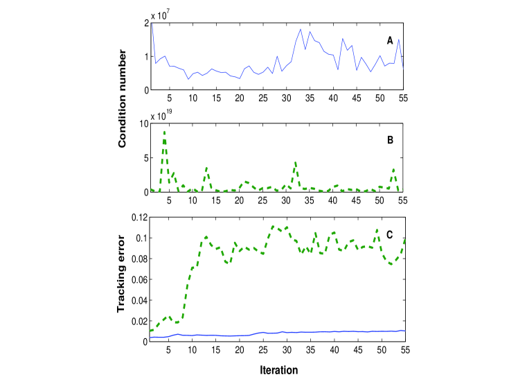
Fig. 5: Comparison of MOTC of a set of 40 observables from four measurement bases for a full-rank nondegenerate mixed initial state $\rho(0)$ and for a pure initial state; the lowest eigenstate $E_{1}$, $|\psi_{1}\rangle$ of $H_{0}$). A) $\Gamma$ matrix condition numbers for thermal $\rho(0)$; B) $\Gamma$ matrix condition numbers for pure $\rho(0)$; C) Associated tracking errors (solid = thermal, dashed = pure).

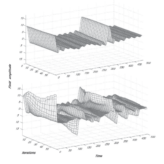
Fig. 6: Evolution of the control field during MOTC with different numbers of measurement bases (system (34)). Top: 5 observables (1 measurement basis); Bottom: 15 observables (2 measurement bases). $\varepsilon_{0}(t)$ was of the form (40); $\rho(0)$ was a full-rank, nondegenerate mixed state.

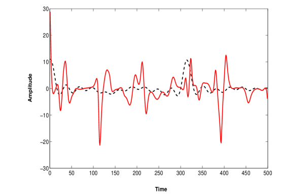
Fig. 7: Superimposition of the optimal control fields identified by MOTC for $5$ (dashed) and $20$ (solid) observable control problems. $\varepsilon_{0}(t)$ was of the form (40); $\rho(0)$ was a full-rank, nondegenerate mixed state. Observables were drawn successively from mutually unbiased measurement bases as described in equation (32).

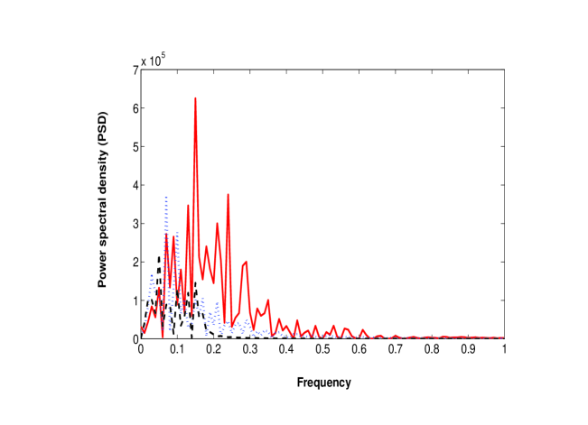
Fig. 8: Fourier power spectra of optimal control fields obtained by MOTC tracking for various numbers of observables $m$. The spectra for $m=5$ (dashed) and $m=20$ (solid), corresponding to the fields in Fig. 7, are shown alongside the spectrum for $m=15$ (dotted).

Greater numbers of orthogonal observables can be effectively tracked for state preparation $\rho(0)$ of higher rank. A full set of observables from multiple measurement bases (or more generally, $m\leq 2Nn-n^{2}$ orthogonal observables) can be effectively tracked for state preparation of $\rho(0)$ with rank $n$, according to equation (19).

Figs. 4A and B indicate that for $m=40$, the $\Gamma$ condition numbers for thermal $\rho(0)$ are significantly lower than those for pure $\rho(0)$. It should be possible to track 40 observables without significant numerical errors occurring due to singularity of the MOTC Gramian. 40 observables can be tracked through measurements in four bases. For this purpose, we employed the $r=0,1,2,3$ MUB bases given by equation (32). The $\Gamma$ condition numbers and associated tracking errors are presented in Fig. 5A,C (solid trace). Despite uniformly higher condition numbers, singularity is not a limiting factor when $\rho(0)$ is thermal; the error correction methods described in section V suffice to maintain the desired optimization trajectory.

For $\rho(0)$ being a pure state, the number of observables that can be simultaneously tracked along arbitrary paths while avoiding $\Gamma$-matrix singularities is lowest. According to Fig. 4, the $\Gamma$-matrix for tracking 40 observables for $\rho(0)$ being pure should be effectively singular. This leads to unacceptably large tracking errors and deviation from the expected path, as shown in Fig. 5C. Indeed, based on the analytical relation (19), it should not be possible to track a full set of observables from more than two measurement bases when $\rho(0)$ is pure. In these cases, search algorithms based on scalar objective optimization, such as the gradient, may be preferred. Nonetheless, as described in Section III, gradient search will generally not effectively locate points on the Pareto front for arbitrary sets of multiple observables.

The evolution of control fields along the optimization trajectory for increasing numbers of observables sheds light on the impact of multiple observable objectives on the control landscape. Fig. 6 compares the control field evolutions for $m=5$ and $m=15$ MOTC, with the track $\textbf{w}_{s}$ given by (30) between $U_{0}$ and a target propagator lying on the global maximum manifold $\mathcal{M}_{1}^{\max}$ for the first observable. At each step, the two fields reside on the same level set of the first observable, but generally deviate increasingly from each other on the domain $\mathcal{U}(N)$. The imposition of additional observable constraints delimits each successive level set such that it contains a smaller set of more complex fields. Fig. 7 isolates and compares the optimal fields obtained by $m=5$ and $m=20$ MOTC. The power spectra of the optimal control fields for $m=5$, $m=15$ and $m=20$ are shown in Fig. 8. Note that although these fields lie on the same level set of a single observable, they are more diverse than those in Fig. 3, which lie on distinct submanifolds of the Pareto front $\mathcal{P}_{w}^{\varepsilon}$. Since control of more orthogonal observables requires control over more independent parameters of the unitary propagator $U(T)$, the latter problem imposes more constraints on the permissible dynamics over $0\leq t\leq T$.

Note that all the MOTC variants in this section (control of up to 40 observables) can be implemented through measurements of four or fewer full-rank, nondegenerate observables in mutually unbiased measurement bases.

VII Discussion

To date, the majority of quantum optimal control experiments (OCE) have been implemented with adaptive (e.g., genetic) search algorithms, which require only measurement of the expectation value of an observable at the final dynamical time for each successive control field. Recently, gradient flow algorithms have been implemented in OCE studies, based on the finding that quantum control landscapes are devoid of suboptimal traps Roslund and Rabitz (2008), and the observation in computer simulations that gradient-based algorithms converge more efficiently than genetic algorithms. Similar conclusions may be drawn about search algorithms for quantum multiobservable control. Whereas in generic multiobjective optimization problems, the existence of local traps typically requires the use of stochastic methods, the inherent monotonicity of quantum control landscapes enables more efficient deterministic algorithms for multiobjective quantum control. Quantum multiobservable tracking control (MOTC) is an example of such an algorithm.

Efficient control algorithms are especially important in the context of quantum Pareto optimization, since the tradeoff between observable objectives in such control problems renders the problem of identifying optimal control fields on the Pareto front via stochastic algorithms much more expensive than the analogous problem of single observable control. Moreover, in quantum Pareto optimization, it is generally nontrivial to parameterize a family of scalar objective functions whose maxima are all (weak) Pareto optima, as demonstrated in section III. Promising successes have been reported in the application of multiobjective evolutionary algorithms (MOEA), which avoid this obstacle, to quantum Pareto optimal control problems involving a limited number of quantum observables $m$ Bonacina et al. (2007). However, the convergence time of such algorithms scales unfavorably with system size due to the computational expense of sorting nondominated solutions Deb et al. (2002). By contrast, apart from the overhead costs of initial state estimation and online measurements of observable expectation values, the convergence time of MOTC does not scale with the number of observables optimized.

In quantum multiobservable maximization problems, it is particularly efficient to first identify points on the kinematic Pareto front $\mathcal{P}_{w}^{U}$ of the multiobservable optimization problem, which requires knowledge or estimation of the initial density matrix $\rho(0)$ of the quantum system. In the case that $\rho(0)$ is not a thermal mixed state, it can be determined by the method of maximal likelihood estimation (MLE) of quantum states Banaszek et al. (1999). Once $\rho(0)$ is known, the Pareto optima on $\mathcal{U}(N)$ can be sampled efficiently using the methods described in Section III. Observable tracking can then be applied in open loop quantum control experiments to locate optimal control fields $\varepsilon^{*}(t)$ on the dynamic Pareto front $\mathcal{P}_{w}^{\varepsilon}$. The local vicinity of each $\varepsilon^{*}(t)$ can subsequently be explored to identify controls with the most favorable dynamic properties.

Experimental observable expectation value tracking requires an extension of gradient flow methods that have already been applied in the laboratory Roslund and Rabitz (2008). Specifically, instead of following the path of steepest ascent, the control field is updated in a direction that in the first-order approximation would produce the next observable track value. In principle, the ability to follow the path of steepest ascent for single observable maximization should be extensible to following arbitrary trajectories across multiobservable control landscapes. When applied in conjunction with signal averaging, statistical estimation of the gradient - employing as few 30 sampled points as per iteration - has been found to confer adequate accuracy and robustness to laser noise in single observable gradient flow algorithms. In practice, experimental multiobservable tracking may demand additional robustness to noise, due to the smaller number of control fields that are consistent with any given point along the track. Experimental error correction, described in Section IV and applied numerically in Section VI, may therefore be essential for these applications. Our goal in this paper has been to lay the theoretical foundations for quantum Pareto optimal control and to illustrate its implementation under ideal conditions. Numerical studies that simulate the effects of control field noise Shuang and Rabitz (2004) on MOTC will be reported in a separate work.

The eigenvalue spectrum of the initial density matrix $\rho(0)$ affects the combinations of observable expectation values that can be simultaneously achieved and the nonsingularity of the multiobservable control Gramian. Tracking a vector $\vec{\Phi}(s)$ of $m$ orthogonal observable expectation values rarely encounters singularities originating in lack of local controllability, if $m\ll N^{2}-1$. However, for the greater number of observables that must be controlled in complex Pareto optimization or state preparation problems, the MOTC Gramian is more prone to becoming ill-conditioned. This effect can be alleviated by carefully tuning the initial guess for the control field.

The additional overhead required for multiobservable tracking, relative to stochastic algorithms, can be mitigated by the development of efficient estimators of multiobservable control gradients. We have presented simple measurement techniques, including the use of mutually unbiased measurement bases, that can dramatically improve MOTC efficiency for large numbers of observables. Still, the methodology for gradient estimation described in section IV does not exploit the statistical correlation of components of the multiobservable gradient (5), which originates in the correlation between elements of $\rho(0)$. Future work should investigate the application of MLE to generate more accurate estimates of the multiobservable gradient for an equivalent number of observable measurements. In addition, it is important to examine the impact of quantum decoherence - which produces nonunitary dynamics described by Kraus operators - on the efficiency of multiobservable tracking.

Appendix A Characterization of Pareto optimal submanifolds

In order to qualitatively assess the likelihood of the gradient flow (6) converging to a weak Pareto optimum where the expectation value of observable $k$ is maximized, the dimensions of $\mathcal{I}_{k,M}^{\max,\max}=\mathcal{M}_{k}^{\max}\bigcap\mathcal{M}_{M}^{\max}$ and $\mathcal{M}_{M}^{\max}$ may be compared. If the two dimensions are equal, there is a finite chance of the gradient flow converging to a Pareto optimum. Otherwise, although the gradient flow may converge arbitrarily close to a Pareto optimum, the attractor of the flow will not be in $\mathcal{P}_{w}^{(U,\varepsilon)}$ and the likelihood of approaching within a fixed radius of a Pareto optimal point will generally be diminished. In this Appendix we present a few results regarding the intersections of the critical submanifolds of the observable objective functions (2), to facilitate such an analysis. As a special case, we also derive the conditions guaranteeing convergence to a weak Pareto optimum given in Lemma 1.

Denote by $\tilde{\Theta}_{a}$ the diagonal form of $\Theta_{a}$ in a basis $S_{a}$ where its eigenvalues are arranged in increasing order; i.e., $\tilde{\Theta}_{a}\equiv S_{a}^{{\dagger}}\Theta_{a}S_{a}=diag\{\gamma_{a(1)},\cdots,\gamma_{a(1)};\cdots;\gamma_{a(s_{a})},\cdots,\gamma_{a(s_{a})}\}$, according to the convention in Section III. Set the diagonal matrix $\tilde{\Theta}_{b}\equiv S_{a}^{{\dagger}}\Theta_{b}S_{a}=S_{a}^{{\dagger}}S_{b}\cdot diag\{\gamma_{b(1)},\cdots,\gamma_{b(1)};\cdots;\gamma_{b(s_{b})},\cdots,\gamma_{b(s_{b})}\}\cdot S_{b}^{{\dagger}}S_{a}.$ Let $\mathcal{U}(\textbf{m}_{b}^{\prime})=S_{a}^{{\dagger}}S_{b}\mathcal{U}(\textbf{m}_{b})S_{b}^{{\dagger}}S_{a}$, where $\mathcal{U}(\textbf{m}_{b})$ is defined as in Section III.

We first obtain an upper bound on $\mathrm{dim~{}}\mathcal{I}_{a,b}^{ij}$. For any observable $\Theta_{a}$, it was shown in Wu et al. (2008) that the dimension of the critical manifold $\mathcal{M}_{a}^{i}$ of $\Phi_{a}$ is given by

$$\mathrm{dim~{}}\mathcal{M}_{a}^{i}=\sum_{x=1}^{r}n_{x}^{2}+\sum_{y=1}^{s_{a}}m_{ay}^{2}-\sum_{x=1}^{r}\sum_{y=1}^{s_{a}}v_{xy}^{2},$$ (41)

where the $v_{xy}$ are overlap numbers that denote the number of positions where the eigenvalues $\gamma_{ax}$ and $\gamma_{ay}$ appear simultaneously in $\tilde{\rho}(0)$ and $\tilde{\Theta}_{a}$, and the $n_{x}$, $m_{ky}$ are defined as in Section III. Then, we have $\mathrm{dim~{}}\mathcal{I}_{a,b}^{ij}\leq{\min}\left\{\mathrm{dim~{}}\mathcal{M}_{a}^{i},\mathrm{dim~{}}\mathcal{M}_{b}^{j}\right\}$ for the upper bound.

Further analytical characterization of $\mathcal{I}_{a,b}^{ij}=\mathcal{M}_{a}^{i}\bigcap\mathcal{M}_{b}^{j}$, including a lower bound on its dimension, is possible when the two observables $\Theta_{a}$ and $\Theta_{b}$ commute. According to equation (10) we have $\mathcal{M}_{a}^{i}\bigcap\mathcal{M}_{b}^{j}=\mathcal{U}(\textbf{n})\pi^{i}\mathcal{U}(\textbf{m}_{a})\bigcap\mathcal{U}(\textbf{n})\pi^{j}\mathcal{U}(\textbf{m}_{b}^{\prime})$ for any $\pi^{i}\in\mathcal{D}_{a}^{i}$, $\pi^{j}\in\mathcal{D}_{b}^{j}$. This can be expressed

$$\left\{\bigcup_{\pi\in\mathcal{D}_{\cap}^{ij}}\mathcal{U}(\textbf{n})\pi\left(\mathcal{U}(\textbf{m}_{a})\cap\mathcal{U}(\textbf{m}_{b}^{\prime})\right)\right\}~{}~{}\bigcup~{}~{}\left\{\bigcup_{\pi^{i}\not\in\mathcal{D}_{\cap}^{ij}~{}\lor~{}\pi^{j}\not\in\mathcal{D}_{\cap}^{ij}}\mathcal{U}(\textbf{n})\pi^{i}\mathcal{U}(\textbf{m}_{a})~{}\cap~{}\mathcal{U}(\textbf{n})\pi^{j}\mathcal{U}(\textbf{m}_{b}^{\prime})\right\},$$

where $\mathcal{D}_{\cap}^{ij}\equiv\mathcal{D}_{a}^{i}\cap\mathcal{D}_{b}^{j}$. The first term in this expression can be written $\{U\pi V~{}|~{}U\in\mathcal{U}(\textbf{n});~{}V\in\mathcal{U}(\textbf{m}_{a})\cap\mathcal{U}(\textbf{m}_{b}^{\prime});~{}\pi\in\mathcal{D}_{\cap}^{ij}\}$. Denote the Lie subgroup $\mathcal{U}(\textbf{m}_{a})~{}\cap~{}\mathcal{U}(\textbf{m}_{b}^{\prime})$ of $\mathcal{U}(N)$ by $\mathcal{U}(\textbf{P})$. Then, we have

$$\bigcup_{\pi\in\mathcal{D}_{\cap}^{ij}}\mathcal{U}(\textbf{n})~{}\pi~{}\mathcal{U}(\textbf{P})~{}\subseteq~{}\mathcal{I}_{a,b}^{ij}.$$ (42)

Let us partition the set $\mathcal{D}_{\cap}^{ij}$ with the equivalence relation $\sim$ defined by $\pi_{1}\sim\pi_{2}$ if $\pi^{2}=U\pi^{1}V,$ for $(U,V)\in\mathcal{U}(\mathbf{n})\times\mathcal{U}(\mathbf{P})$. Then it is straightforward to show that $\pi$’s in different equivalence classes with respect to $\sim$ label disconnected submanifolds of $\bigcup_{\pi\in\mathcal{D}_{\cap}^{ij}}\mathcal{U}(\textbf{n})\pi\mathcal{U}(\textbf{P})$. $\mathcal{U}(\textbf{P})$ can be written $\mathcal{U}(p_{11})\times\cdots\times\mathcal{U}(p_{s_{a}s_{b}})$, where the $p_{xy}$ are overlap numbers that denote the number of positions where the eigenvalues $\gamma_{ax}$ and $\gamma_{by}$ appear simultaneously in $\tilde{\Theta}_{a}$ and $\tilde{\Theta}_{b}^{\prime}$. Together, these overlap numbers form a contingency table Wu et al. (2008), with rows indexed by $x$ and columns indexed by $y$. The row sums are $\sum_{y=1}^{s_{b}}p_{xy}=m_{ax}$ and the column sums are $\sum_{x=1}^{s_{a}}p_{xy}=m_{by}$.

Based on these results we can now derive conditions guaranteeing convergence of (6) to a weak Pareto optimum. We have $\mathcal{M}_{b}^{j}\subseteq\mathcal{M}_{a}^{i}$ if there is just one nonzero entry in each column of the contingency table (such that each $S_{a}^{{\dagger}}S_{b}~{}\mathcal{U}(m_{by})~{}S_{b}^{{\dagger}}S_{a}\subseteq\mathcal{U}(m_{ax})$ for just one $x$, hence $\mathcal{U}(\textbf{P})=\mathcal{U}(\textbf{m}_{b}^{\prime})$), and $\mathcal{D}_{b}^{j}\subseteq\mathcal{D}_{a}^{i}$ (such that $\mathcal{D}_{a}^{i}\bigcap\mathcal{D}_{b}^{j}=\mathcal{D}_{b}^{j}$); then, $\mathcal{I}_{a,b}^{ij}=\mathcal{M}_{b}^{j}$. In this case we have the first equality in equation (42) and all $\pi\in\mathcal{D}_{\cap}^{ij}$ belong to the same equivalence class with respect to $\sim$. If we set $\Theta_{a}=\Theta_{k}$ and $\Theta_{b}=\Theta_{M}$, this proves the conditions guaranteeing convergence to $\mathcal{P}_{w}^{(U,\varepsilon)}$ in Lemma 1. $\blacksquare$

We now obtain a lower bound on $\mathrm{dim~{}}\mathcal{I}_{a,b}^{ij}$ in the case of commuting $\Theta_{a}$, $\Theta_{b}$. Define $F_{\pi}(P,Q):\pi\rightarrow P\pi Q,$ where $(P,Q)\in\mathcal{U}(\textbf{n})\times\mathcal{U}(\textbf{P})$, and let $stab~{}(F_{\pi})$ denote the set of all $(U,V)\in\mathcal{U}(\textbf{n})\times\mathcal{U}(\textbf{P})$ such that $F_{\pi}(U,V)=U\pi V=\pi$. It is straightforward to verify Wu et al. (2008) that $stab~{}(F_{\pi})=\mathcal{U}(\textbf{n})~{}\bigcap~{}\pi^{{\dagger}}~{}\mathcal{U}(\textbf{P})~{}\pi$. The latter may be written $\mathcal{U}(\textbf{Q})=\mathcal{U}(q_{111})\times\cdots\times\mathcal{U}(q_{rs_{a}s_{b}})$, where the overlap numbers $q_{xyz}$ denote the number of positions where the eigenvalue $\lambda_{i}$ appears simultaneously with $\gamma_{ay}$ and $\gamma_{bz}$, after the permutation $\pi$ has been applied to $\tilde{\Theta}_{a},~{}\tilde{\Theta}_{b}^{\prime}$. It was shown in Wu et al. (2008) that any manifold of the type $\mathcal{U}(\textbf{n})~{}\pi~{}\mathcal{U}(\textbf{P})$ has dimension $\mathrm{dim~{}}\mathcal{U}(\textbf{n})+\mathrm{dim~{}}\mathcal{U}(\textbf{P})-\mathrm{dim~{}}stab(F_{\pi})$. Given that the dimension of $\mathcal{U}(N)$ is $N^{2}$, the lower bound on the dimension of the intersection submanifold is thus

$$\mathrm{dim~{}}\mathcal{I}_{a,b}^{ij}\geq\max_{\pi\in\mathcal{D}_{\cap}^{ij}}\left\{\sum_{x=1}^{r}n_{x}^{2}+\sum_{x=1}^{s_{a}}\sum_{y=1}^{s_{b}}p_{xy}^{2}-\sum_{x=1}^{r}\sum_{y=1}^{s_{a}}\sum_{z=1}^{s_{b}}q_{xyz}^{2}\right\}.$$ (43)

In the case that the observables commute, we therefore have both analytical lower and upper bounds on $\mathrm{dim~{}}\mathcal{I}_{k,M}^{\max,\max}$, whereas if they do not commute, we have only the upper bound. If the upper bound is less than $\mathrm{dim~{}}\mathcal{M}_{M}^{\max}$, then the chance of the flow converging to $\mathcal{P}_{w}^{(U,\varepsilon)}$ is infinitesimally small (although it may approach arbitrarily close). The lower bound is most useful when it equals $\mathrm{dim~{}}\mathcal{M}_{M}^{\max}$, in which case there is a finite chance that the flow will converge to $\mathcal{P}_{w}^{(U,\varepsilon)}$.

References

- Banaszek et al. (1999) K. Banaszek, G. D’Ariano, M. Paris, and M. Sacchi, Physical Review A 61, 010304 (1999).
- Bonacina et al. (2007) L. Bonacina, J. Extermann, A. Rondi, V. Boutou, and J. Wolf, Phys. Rev. A 76, 023408 (2007).
- Weber et al. (2007) S. M. Weber, F. Sauer, M. Plewicki, A. Merli, L. Wöste, and A. Lindinger, J. Mod. Opt. 54, 2659 (2007).
- Chakrabarti et al. (2008) R. Chakrabarti, R. Wu, and H. Rabitz, Phys. Rev. A, to appear (2008), eprint eprint arXiv:0805.1556 [quant-ph].
- Li et al. (2002) B. Q. Li, G. Turinici, V. Ramakrishna, and H. Rabitz, J. Phys. Chem. B 106, 8125 (2002).
- Li et al. (2005) B. Q. Li, H. Rabitz, and J. P. Wolf, J. Chem. Phys. 122, 154103 (2005).
- Chakrabarti and Rabitz (2007) R. Chakrabarti and H. Rabitz, Int. Rev. Phys. Chem. 26, 671 (2007).
- Hillermeier (2001) C. Hillermeier, Nonlinear multiobjective optimization: a generalized homotopy approach (Birkhauser, Basel, 2001).
- Statnikov and Matusov (1990) R. B. Statnikov and J. B. Matusov, Multicriteria Optimization and Engineering (Springer-Verlag, New York, 1990).
- Levis et al. (2001) R. Levis, G. Menkir, and H. Rabitz, Science 292, 709 (2001).
- Rabitz et al. (2006) H. Rabitz, M. Hsieh, and C. Rosenthal, J. Chem. Phys. 124, 204107 (2006).
- Ho and Rabitz (2006) T.-S. Ho and H. Rabitz, J. Photochem. Photobiol. A 180, 226 (2006).
- Lin (1976) J. G. Lin, IEEE Trans. Autom. Control 21, 641 (1976).
- Wu et al. (2008) R. Wu, H. Rabitz, and M. Hsieh, J. Phys. A 41, 015006 (2008).
- Deb et al. (2002) K. Deb, A. Pratap, S. Agarwal, and T. Meyarivan, IEEE Trans. Evol. Comp. 6, 182 (2002).
- Knowles and Corne (1999) J. Knowles and D. Corne, in Proceedings of the 1999 Congress on Evolutionary Computation (IEEE Press, Piscataway, NJ, 1999), pp. 98–105.
- Zitzer and Thiele (1999) E. Zitzer and L. Thiele, in Parallel problem solving from nature, edited by A. E. Eiben, T. Back, M. Schoenauer, and H.-P. Schwefel (Springer-Verlag, Berlin, Germany, 1999), pp. 292–301.
- Ramakrishna et al. (1995) V. Ramakrishna, M. V. Salapaka, M. Dahleh, H. Rabitz, and A. Peirce, Phys. Rev. A 51, 960 (1995).
- Buzek et al. (1999) V. Buzek, G. Drobny, R. Derka, G. Adam, and H. Wiedemann, Chaos, Solitons and Fractals 10, 981 (1999).
- Rothman et al. (2006) A. Rothman, T. Ho, and H. Rabitz, Phys. Rev. A 73, 053401 (2006).
- Pechen et al. (2008) A. Pechen, D. Prokhorenko, R. Wu, and H. Rabitz, J. Phys. A 41, 045205 (2008).
- Dominy and Rabitz (2008) J. Dominy and H. Rabitz, J. Phys. A 41, 205305 (2008).
- Uhlmann (1976) A. Uhlmann, Rep. Math. Phys. 9, 273 (1976).
- Wootters and Fields (1989) W. K. Wootters and B. D. Fields, Ann. of Phys. 191, 363 (1989).
- Roslund and Rabitz (2008) J. Roslund and H. Rabitz, To be submitted (2008).
- Albertini and D’Alessandro (2003) F. Albertini and D. D’Alessandro, IEEE Trans. Autom. Cont. 48, 1399 (2003).
- Shuang and Rabitz (2004) F. Shuang and H. Rabitz, J. Chem. Phys. 121, 9270 (2004).