1D-FFLO state in the absence of time-reversal symmetry breaking

Abstract

A novel route to a one-dimensional Fulde-Ferrell-Larkin-Ovchinnikov (1D-FFLO) state in the absence of broken time-reversal symmetry is proposed in this paper. At present such a state may be encouraged in a clean AlAs quantum wire. Using the AlAs quantum wire as an example it is shown using bosonization and the renormalization group approach that the 1D-FFLO state can arise due to a combination of Coulomb interactions and the unique bandstructure arrangement of the AlAs quantum wire. The present theoretical proposal is very general and is applicable to other systems with similar fermionic interaction terms.

A superconducting state with a finite pairing momentum had been long proposed by Fulde and Ferrell Fulde and Ferrell (1964), and Larkin and Ovchinnikov Larkin and Ovchinnikov (1965). Presently this state is known as the Fulde-Ferrell-Larkin-Ovchinnikov (FFLO) (or LOFF) state. The FFLO state is widely realized from condensed matter systems to high energy physics Casalbuoni and Nardulli (2004). In a FFLO state Cooper pairs with a nonzero center-of-mass momentum are encouraged in the presence of an external magnetic field. The central physical ingredient of the originally studied FFLO state is based on the idea that Cooper pairs in a spin-singlet superconductor are composed of fermions with opposite spins. In the presence of a magnetic field these electrons couple to the external applied field through the Zeeman coupling. This in turn tends to polarize the electrons along the direction of the magnetic field and allows the system to gain polarization energy. However, the pairing of opposite spins is favorable for condensation energy. Due to these competing tendencies the superconducting state undergoes a transition to the FFLO state with a finite pairing momentum and eventually enters the normal state as the magnetic field is further increased Fulde and Ferrell (1964); Larkin and Ovchinnikov (1965).

There have been several theoretical proposals that such a state may be achievable in heavy fermion systems and organic and cuprate superconductors Gloos et al. (1993); Tachiki et al. (1996); Modler et al. (1996); Gegenwart et al. (1996); O’Brien et al. (2000); Singleton et al. (2000); Singh and Mazin (2002); Tanatar et al. (2002); Krawiec et al. (2004), as well as in cold atomic gases Liu and Wilczek (2003), 1D Kondo lattice Zachar et al. (1996), and even nuclear and quark matter Casalbuoni and Nardulli (2004). The field has been energized by recent experimental evidence of the FFLO state in the heavy fermion superconductor CeCoIn₅ Cui et al. (2006); Radovan et al. (2003); Bianchi et al. (2003). Recent theoretical progress has indicated that the state may be achievable through applied current rather than an applied field Doh et al. (2006). The original prediction as well as the more recent ones rely on introducing a magnetic field (whether externally or as an effective internal mean field Machida and Nakanishi (1984)), or using some other perturbation in order to create the unequal Fermi surfaces necessary to generate finite-momentum pairing.

In this paper, a novel route to a 1D-FFLO state is proposed in the absence of a magnetic field or any other external perturbation with the AlAs system as an example. This system was recently fabricated and investigated by Moser et al. Moser et al. (2005, 2006). In such a system it should be possible to induce an FFLO state due to the interplay of Coulomb interaction effects with the specific bandstructure of the AlAs quantum wire, which includes a unique inter-valley umklapp scattering process that is present at all densities.

\psfrag{k}{k}\psfrag{E}{E}\psfrag{umk}{$\frac{k_{U}}{2}$}\psfrag{A}{A}\psfrag{B}{B}\includegraphics[width=205.96883pt]{bandstructure.EPS}

Figure 1: Schematic of the 1D bandstructure in the AlAs quantum wire of Ref. Moser et al., 2005. The bandstructure has two degenerate subbands at the lowest densities, leading to four Fermi points. In addition, the band minima are separated by half an umklapp vector, $k_{U}/2$, giving rise to umklapp interactions which are present at all fillings. The effective dispersion can be linearized so that the Fermi points, represented by black dots on the figure, are at $k^{A\pm}_{F}=-\frac{k_{U}}{4}\pm k^{o}_{F}$ and $k^{B\pm}_{F}=\frac{k_{U}}{4}\pm k^{o}_{F}$ where $k_{U}$ is the umklapp vector, and $k_{F}^{o}$ is the magnitude of the Fermi wavevector measured from the bottom of each band.

A schematic of the AlAs quantum wire bandstructure is shown in Fig. 1 Moser et al. (2005, 2006). While bulk AlAs has three degenerate bands, the growth direction and cleavage planes chosen in fabricating the wire leave two degenerate valleys at low energy. In the effective one-dimensional bandstructure, this leads to two degenerate nonoverlapping bands separated by half an umklapp vector, as shown in Fig. 1. Because the momenta of the two band minima are related by half an umklapp vector, there is a class of umklapp excitations unique to this bandstructure which exists at all densities. Because there are four Fermi points, the bandstructure supports several fermionic scattering processes. We retain only those scattering terms which are relevant in a renormalization group sense.

\psfrag{E}{E}\psfrag{k}{k}\includegraphics[width=252.94499pt]{umklappcooper.EPS}

Figure 2: Representative inter-valley umklapp scattering process which is responsible for encouraging the 1D-FFLO state. In the process which is shown, a pair of left and right movers from the A band scatters into a pair of left and right movers in the B band by absorbing an umklapp vector. This is an umklapp process which is present at all densities.

In a quantum wire electrons are quantum mechanically confined to move along one direction with their motion in the remaining transverse directions confined via a potential, $V_{conf}(\vec{r_{\perp}})$, where $\vec{r}_{\perp}=(y,z)$ denotes the transverse coordinates of quantization. Electron-electron interactions within the wire are described by $U(\vec{r}$) which is purely repulsive. The Hamiltonian is a sum of two independent terms in the transverse and longitudinal directions with the result that the wavefunction (and therefore the correlation functions) can be decomposed as a product of $\phi(\vec{r}_{\perp})$ and $\psi_{s}(x)$ where $\phi(\vec{r}_{\perp})$ is the orthogonal wavefunction of transverse quantization of the two degenerate bands ($X$ and $Y$ valleys) and $\psi_{s}(x)$ the longitudinal part. In order to describe the physics along the longitudinal direction we now promote the wavefunction, $\psi_{s}(x)$, to the level of a field operator (for a field theoretic description) responsible for creating and annihilating the electrons taking part in the various scattering processes. With this in mind the second quantized Hamiltonian suitable for the purposes of our study is

$$H=\sum_{s}\int d^{3}r\Psi^{{\dagger}}_{s}(\vec{r})\left(-\frac{1}{2m}\vec{\nabla}^{2}_{r}-\mu+V_{conf}(\vec{r}_{\perp})\right)\Psi_{s}(\vec{r})$$

$$+\frac{1}{2}\sum_{s,s^{{}^{\prime}}}\int d^{3}rd^{3}r^{{}^{\prime}}U(\vec{r}-\vec{r^{{}^{\prime}}})\Psi^{{\dagger}}_{s}(\vec{r})\Psi^{{\dagger}}_{s^{{}^{\prime}}}(\vec{r}^{{}^{\prime}})\Psi_{s^{{}^{\prime}}}(\vec{r}^{{}^{\prime}})\Psi_{s}(\vec{r})$$

where $\Psi_{s}(\vec{r})=\phi(\vec{r}_{\perp})\psi_{s}(x)$ is now the field operator for an electron species of spin $s=\{\uparrow,\downarrow$}, and $\mu$ is the chemical potential in the leads. Because the low energy, long wavelength excitations occur in the vicinity of the Fermi points (see Fig. 2) a further decomposition is possible with $\Psi_{s}(\vec{r})=\phi(\vec{r}_{\perp})(\psi_{As}(x)+\psi_{Bs}(x))$. The coordinate $x$ is in the long direction of the wire. The longitudinal part of the field can be naturally expanded in terms of the right- and left- moving excitations, $R_{ns}(x)$ and ${L}_{ns}(x)$, respectively, residing around the Fermi points of the two bands (indicated by the black dots in Fig. 1) with $\psi_{As}(x)=R_{As}(x)e^{ik^{A+}_{F}x}+L_{As}(x)e^{ik^{A-}_{F}x}$ and $\psi_{Bs}(x)=R_{Bs}(x)e^{ik^{B+}_{F}x}+L_{Bs}(x)e^{ik^{B-}_{F}x}$. The band index is $n=A,B$ and the Fermi momenta are defined by $k^{A\pm}_{F}=-\frac{k_{U}}{4}\pm k^{o}_{F}$ and $k^{B\pm}_{F}=\frac{k_{U}}{4}\pm k^{o}_{F}$ where $k_{U}$ is the umklapp vector, and $k_{F}^{o}$ is the magnitude of the Fermi wavevector measured from the bottom of each band, as shown in Fig. 1.

The low energy properties of the interacting 1D electron gas can now be conveniently described within the framework of the bosonization technique Giamarchi (2004). Within this approach, the fermionic field operators can be written in terms of bosonic fields $\phi_{n\nu}=(\phi_{n\uparrow}\pm\phi_{n\downarrow})/\sqrt{2}$ and $\theta_{n\nu}=(\theta_{n\uparrow}\pm\theta_{n\downarrow})/\sqrt{2}$, where $\nu=\rho,\sigma$ (the charge and spin modes) correspond to the $\pm$ combination, $s=\{\uparrow,\downarrow$} is the spin index and $n=A,B$ is the band index. The bosonic fields satisfy the commutation relation [$\phi_{n\nu}(x),\partial_{x^{{}^{\prime}}}\theta_{n^{{}^{\prime}}\nu^{{}^{\prime}}}(x^{{}^{\prime}})$]=i$\pi\delta(x-x^{{}^{\prime}})\delta_{\nu,\nu^{{}^{\prime}}}\delta_{n,n^{{}^{\prime}}}$ with $\hbar$ set equal to one. We then have

$${R}_{ns}(x)=\frac{\eta_{Rns}}{\sqrt{2\pi\alpha}}e^{i\sqrt{\pi\over 2}[\theta_{n\rho}(x)-\phi_{n\rho}(x)+s(\theta_{n\sigma}(x)-\phi_{n\sigma}(x))]}$$ (2)

and,

$${L}_{ns}(x)=\frac{\eta_{Lns}}{\sqrt{2\pi\alpha}}e^{i\sqrt{\pi\over 2}[\theta_{n\rho}(x)+\phi_{n\rho}(x)+s(\theta_{n\sigma}(x)+\phi_{n\sigma}(x))]}$$ (3)

where $\alpha$ is the short distance cutoff, and $\eta_{Rns}$ and $\eta_{Lns}$ are the Klein factors for the right- and left- moving fields of band $n$ with species of spin $s$. They are required to preserve the anti-commutation relations of the fermionic fields. The convenient field variables for the Hamiltonian in our problem will be a linear combination of the boson fields constructed out of the two bands. We define the transformation to a symmetric and an anti-symmetric basis as $\phi^{\pm}_{\nu}=\frac{1}{\sqrt{2}}(\phi_{A\nu}\pm\phi_{B\nu})$ and $\theta^{\pm}_{\nu}=\frac{1}{\sqrt{2}}(\theta_{A\nu}\pm\theta_{B\nu})$.

Upon bosonization and subsequent transformation the parts of the Hamiltonian corresponding to kinetic energy lead to harmonic terms in the symmetric and the anti-symmetric bosonic fields $(\phi^{\pm}_{\nu}$ and $\theta^{\pm}_{\nu})$. The intraband interactions and the interband interactions, however, generate both cosine interaction terms and harmonic terms umk . The Hamiltonian, $H$, can then be written in the following canonical form.

$$H=\frac{1}{2}\sum_{\nu=\rho,\sigma}\int dR\bigg{[}v^{\pm}_{\nu}K^{\pm}_{\nu}(\partial_{R}\theta^{\pm}_{\nu})^{2}+\frac{v^{\pm}_{\nu}}{K^{\pm}_{\nu}}(\partial_{R}\phi^{\pm}_{\nu})^{2}\bigg{]}+H_{int}~{}.$$ (4)

Here, $R=(x+x^{{}^{\prime}})/2$ is the center-of-mass coordinate of two electrons and $a=x-x^{{}^{\prime}}$ their relative coordinate in the long direction of the quantum wire. In the quadratic part of the Hamiltonian the bare symmetric and anti-symmetric Luttinger parameters, $K^{\pm}_{\nu}$ can be expressed in terms of the original Luttinger parameters $K_{\nu}$. The symmetric and anti-symmetric velocities $v^{\pm}_{\nu}$ can also be expressed in terms of the original velocities $v_{\nu}$. The terms responsible for interactions in the bosonic fields are included in $H_{int}$. There are eleven such interaction terms in the bosonized form. Weak coupling renormalization group (RG) (to second order in the interaction coupling constants) is then used to determine the instabilities of the AlAs quantum wire Balents and Fisher (1996); Schulz (1996); Lin et al. (1998). The corresponding coupled nonlinear differential equations are then solved, using appropriate physical inputs as initial conditions for the RG flow, as discussed below.

The interaction terms which ultimately determine the final phases are

$$\frac{t_{a}}{2\pi^{2}\alpha^{2}}\int dR\cos[\sqrt{4\pi}\phi^{-}_{\rho}]\cos[\sqrt{4\pi}\phi^{+}_{\sigma}]$$ (5)

$$\frac{t_{b}}{2\pi^{2}\alpha^{2}}\int dR\cos[\sqrt{4\pi}\phi^{-}_{\rho}]\cos[\sqrt{4\pi}\phi^{-}_{\sigma}]$$

$$\frac{t_{c}}{2\pi^{2}\alpha^{2}}\int dR\cos[\sqrt{4\pi}\theta^{-}_{\rho}]\cos[\sqrt{4\pi}\phi^{+}_{\sigma}]$$

$$\frac{t_{d}}{2\pi^{2}\alpha^{2}}\int dR\cos[\sqrt{4\pi}\theta^{-}_{\rho}]\cos[\sqrt{4\pi}\phi^{-}_{\sigma}]~{}.$$

The initial values of the coupling constants are set by

$$t_{a}=2\int daM(a)\cos[2k^{o}_{F}a]$$ (6)

$$t_{b}=2\int daM(a)\bigg{(}\cos[2k^{o}_{F}a]-\cos\bigg{[}\frac{k_{U}a}{2}\bigg{]}\bigg{)}$$

$$t_{c}=2\int daM(a)\cos[2k^{o}_{F}a]\cos\bigg{[}\frac{k_{U}a}{2}\bigg{]}$$

$$t_{d}=2\int M(a)\cos\bigg{[}\frac{k_{U}a}{2}\bigg{]}$$

We use a screened Coulomb potential for the interaction kernel, $M(a)=\frac{e^{2}}{4\pi\epsilon}\frac{e^{-(a/d)}}{\sqrt{w^{2}+a^{2}}}$, where $e$ is the electronic charge, $\epsilon=10.9\epsilon_{o}$ is the dielectric constant of AlAs Streetman (1990), and $\epsilon_{o}$ is the permittivity of free space. The width of the quantum wire $w$ provides a short distance cutoff whereas the distance to the back-gate $d$ provides a long distance cutoff.

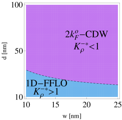
(a)  $n=10^{5}cm^{-1}$

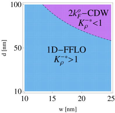
(b)  $n=5\times 10^{4}cm^{-1}$

Figure 3: Variation of $K^{-}_{\rho}$ with distance to the back gate $(d)$ and width of the wire $(w)$, using $L=1\mu m$, $\epsilon=10.9\epsilon_{o}$, and $m^{*}=0.33m_{e}$.

Using input parameters appropriate to the wire, and the expression for the coupling constants, Eq. 6, we can make an estimate for the initial conditions of the RG flow, i.e. the bare values of the coupling constants $t_{i}$. The AlAs quantum wire of Moser et al.Moser et al. (2006, 2005) fabricated using standard design parameters has a transverse size of $w\approx 15nm$ separated from the metallic gate by a distance $d\approx 300nm$. The wire length is $L\approx 1\mu m$, so that $w/d\approx$ 0.05 and $L/d$ = 10/3. The parameters used to estimate $k^{o}_{F}$ for the AlAs bandstructure are as follows: the density of the electrons in the quantum wire $\approx 10^{6}cm^{-1}$ and the effective mass of the electron $m^{*}=0.33m_{e}$ along the long direction where $m_{e}$ is the bare mass of the electron Moser et al. (2006). Experimental evidence Gunawan et al. (2004); Shkolnikov et al. (2002) suggests that spin rotational invariance is not broken in the AlAs quantum wells in the absence of a magnetic field (i.e. spin-orbit coupling is negligible.) Furthermore, since there is no external magnetic field present spin rotational invariance is not broken and we set the initial spin Luttinger parameters $K^{\pm}_{\sigma}$ equal to one.

Given these inputs for the bare parameters, we allow the running coupling constants to flow according to the RG equations with initial conditions for the bare Luttinger parameters $K^{-}_{\rho}<1$ or $K^{-}_{\rho}>1$ together with initial values for $K^{\pm}_{\sigma}$ set equal to one. When one or more coupling constants grows to be of $\mathcal{O}(1)$, we stop the flow. At that point, the fields for the corresponding divergent couplings develop a gap to excitations, and acquire a definite expectation value. This expectation value is then inserted into the correlation functions in order to determine the type of phase this instability represents.

Using this standard analysis, with initial conditions appropriate to the AlAs quantum wire as described above, we find that for the wire fabricated by Moser et al. the coupling constants which diverge are $t_{a}$ and $t_{b}$, leading to a state with divergent $2k^{o}_{F}$-charge-density wave $(CDW)$ correlations. This arises because the relative charge channel flows to an effectively repulsive state, with effective Luttinger parameter $K_{\rho}^{-*}<1$.

Although the bare interactions are (screened) repulsive Coulomb interactions, it is possible for the interactions of the relative charge channel to flow to an effective attractive regime, i.e. $K_{\rho}^{-*}>1$. When this happens, the coupling constants which diverge are $t_{c}$ and $t_{d}$, while $t_{a}$ and $t_{b}$ remain small. From the interaction terms we can then deduce that the dual antisymmetric charge field $\theta_{\rho}^{-}$ gets gapped together with the spin fields $\phi^{\pm}_{\sigma}$. These gapped fields lead to a state with divergent intraband singlet superconductivity correlations with a finite pairing momentum - the 1D-FFLO state. The pairing mechanism in this case is shown in Fig. 2. The diverging interactions allow left and right movers from band “A” to scatter into a left and right mover in band “B” by absorbing an umklapp vector. That is, pairs form within each band in order to take advantage of the lowering of energy possible with umklapp scattering from one band to the other. This is analogous to the spin gap proximity effect mechanism described in Ref. Emery et al., 1997. Because each pair resides within a single valley, the pairs each have a net momentum, $\pm k_{U}/2$, leading to a 1D FFLO state cnt ; Ando et al. (1998).

Phase diagrams showing this transition from $2k^{o}_{F}$-CDW to the FFLO state are shown in Fig. 3. Our calculations indicate that the previously fabricated AlAs QWR of Refs. Moser et al., 2005, 2006 would require extremely low densities (i.e. $n\approx 10^{4}cm^{-1}$) in order to achieve the FFLO state. Such low densities would not only make the behavior of the wire more susceptible to disorder, but it would also require a longer wire in order to achieve a reasonable total number of electrons in the wire. By using an alternate structure with a metallic side gate, it may be possible to make the long distance screening length as small as $d=10-30$ nm Mat . In this case, our calculations indicate that the FFLO state could be achievable for more reasonable densities, on the order of $n\approx 10^{5}cm^{-1}$.

In conclusion, we have proposed a novel route to an FFLO state in 1D. The state should be achievable in AlAs QWR’s for which the bandstructure leads to pairing generated by umklapp pair scattering which is present at all densities. This particular FFLO state is intrinsic to the wire, and does not require an external field or perturbation in order to induce the state. The theoretical proposal is general. It is applicable to other systems with a similar bandstructure where analogous fermionic interaction terms are allowed.

The author wishes to acknowledge Erica W. Carlson for suggesting the problem and additionally wishes to thank Matthew Grayson and Joel Moser for numerous insightful and useful discussions about the aluminum arsenide quantum wire system.

References

- Fulde and Ferrell (1964) P. Fulde and R. A. Ferrell, Phys. Rev. 135, A550 (1964).
- Larkin and Ovchinnikov (1965) A. I. Larkin and Y. N. Ovchinnikov, Sov. Phys. JETP 20, 762 (1965).
- Casalbuoni and Nardulli (2004) R. Casalbuoni and G. Nardulli, Rev. Mod. Phys. 76, 263 (2004).
- Gloos et al. (1993) K. Gloos, R. Modler, H. Schimanski, C. D. Bredl, C. Geibel, F. Steglich, A. I. Buzdin, N. Sato, and T. Komatsubara, Phys. Rev. Lett. 70, 501 (1993).
- Tachiki et al. (1996) M. Tachiki, S. Takahashi, P. Gegenwart, M. Weiden, C. G. M. Lang, F. Steglich, R. Modler, C. Paulsen, and Y. Onuki, Z. Phys. B: Condens. Matter 100, 369 (1996).
- Modler et al. (1996) R. Modler, P. Gegenwart, M. Lang, M. Deppe, M. Weiden, T. Lühmann, C. Geibel, F. Steglich, C. Paulsen, J. L. Tholence, et al., Phys. Rev. Lett. 76, 1292 (1996).
- Gegenwart et al. (1996) P. Gegenwart, M. Deppe, M. Koppen, F. Kromer, M. Lang, R. Modler, M. Weiden, C. Geibel, F. Steglich, T. Fukase, et al., Ann. Phys. 5, 307 (1996).
- O’Brien et al. (2000) J. L. O’Brien, H. Nakagawa, A. S. Dzurak, R. G. Clark, B. E. Kane, N. E. Lumpkin, R. P. Starrett, N. Muira, E. E. Mitchell, J. D. Goettee, et al., Phys. Rev. B 61, 1584 (2000).
- Singleton et al. (2000) J. Singleton, J. A. Symington, M.-S. Nam, A. Ardavan, M. Kurmoo, and P. Day, J. Phys.: Condens. Matter 12, L641 (2000).
- Singh and Mazin (2002) D. J. Singh and I. I. Mazin, Phys. Rev. Lett. 88, 187004 (2002).
- Tanatar et al. (2002) M. A. Tanatar, T. Ishiguro, H. Tanaka, and H. Kobayashi, Phys. Rev. B 66, 134503 (2002).
- Krawiec et al. (2004) M. Krawiec, B. L. Györffy, and J. F. Annett, Phys. Rev. B 70, 134519 (2004).
- Liu and Wilczek (2003) W. V. Liu and F. Wilczek, Phys. Rev. Lett. 90, 047002 (2003).
- Zachar et al. (1996) O. Zachar, S. A. Kivelson, and V. J. Emery, Phys. Rev. Lett. 77, 1342 (1996).
- Cui et al. (2006) Q. Cui, C.-R. Hu, J. Y. T. Wei, and K. Yang, Phys. Rev. B 73, 214514 (2006).
- Radovan et al. (2003) H. A. Radovan, N. A. Fortune, T. P. Murphy, S. T. Hannahs, E. C. Palm, S. W. Tozer, and D. Hall, Nature (London) 425, 51 (2003).
- Bianchi et al. (2003) A. Bianchi, R. Movshovich, C. Capan, P. G. Pagliuso, and J. L. Sarrao, Phys. Rev. Lett. 91, 187004 (2003).
- Doh et al. (2006) H. Doh, M. Song, and H.-Y. Kee, Phys. Rev. Lett. 97, 257001 (2006).
- Machida and Nakanishi (1984) K. Machida and H. Nakanishi, Phys. Rev. B 30, 122 (1984).
- Moser et al. (2005) J. Moser, T.Zibold, S.Roddaro, D.Schuh, M.Bichler, V.Pellegrini, G.Abstreiter, and M.Grayson, Appl. Phys. Lett. 87, 052101 (2005).
- Moser et al. (2006) J. Moser, S. Roddaro, D. Schuh, M. Bichler, V. Pellegrini, and M. Grayson, Phys. Rev. B 74, 193307 (2006).
- Giamarchi (2004) T. Giamarchi, Quantum Physics in One Dimension (Clarendon Press, Oxford, 2004).
- (23) While bosonizing I have used the fact that the exponential . This is true because the electrons in the QWR move in an underlying lattice and their spatial coordinate , where is the lattice spacing in the long direction of the wire and is an integer. When multiplied with the umklapp vector, , and exponentiated the result is .
- Balents and Fisher (1996) L. Balents and M. P. A. Fisher, Phys. Rev. B 53, 12133 (1996).
- Schulz (1996) H. J. Schulz, Phys. Rev. B 53, R2959 (1996).
- Lin et al. (1998) H.-H. Lin, L. Balents, and M. P. A. Fisher, Phys. Rev. B 58, 1794 (1998).
- Streetman (1990) B. G. Streetman, Solid State Electronic Devices (Prentice Hall, 1990), 3rd ed.
- Gunawan et al. (2004) O. Gunawan, Y. P. Shkolnikov, E. P. D. Poortere, E. Tutuc, and M. Shayegan, Phys. Rev. Lett. 93, 246603 (2004).
- Shkolnikov et al. (2002) Y. P. Shkolnikov, E. P. De Poortere, E. Tutuc, and M. Shayegan, Phys. Rev. Lett. 89, 226805 (2002).
- Emery et al. (1997) V. J. Emery, S. A. Kivelson, and O. Zachar, Phys. Rev. B 56, 6120 (1997).
- (31) The 1D-FFLO correlation will NOT arise in carbon nanotubes since the umklapp scattering process is not allowed in the carbon nanotube bandstructure. This is due to the absence of backscattering processes Ando et al. (1998).
- Ando et al. (1998) T. Ando, T. Nakanishi, and R. Saito, J. Phys. Soc. Jpn. 67, 2857 (1998).
- (33) M. Grayson, private communication.