Non-minimal scalar fields in 2D de Sitter and dilaton black holes

Abstract:

We study non-minimal quantum fields in the gravitational field of 2-dimensional dilaton black holes and the de Sitter spacetime. We found that the Green functions for non-minimal massless fields in a particular class of dilaton black holes and in the de Sitter spacetime are almost identical. Using this symmetry exact solutions are derived for quasinormal modes and bound states in these background geometries. The problem of stability of dilaton black holes is discussed.

1 Introduction

Our purpose is to study quantum scalar fields living on the background of a special class of solutions of (1+1)-dimensional dilaton gravity. This class of 2D spacetimes includes a variety of dilaton black holes (BH) such as CGHS solution [1] as well as the de Sitter spacetime. In this paper non-minimality is understood as a presence in the Lagrangian of an interaction term with the scalar curvature rather than with the dilaton. We demonstrate that, although the geometry of black holes is quite different from that of the de Sitter space, the dynamics of quantum non-minimal massless scalar fields does not depend really on this difference. At first sight it looks surprising, since the de Sitter geometry seems to be much more symmetrical than, e.g., the CGHS model, but it happens that for non-minimal fields they look alike. This property provides a tool to translate many quantum effects, which were calculated for the de Sitter space, to the 2D black hole background and vice versa. Quantum fields on the de Sitter background have been studied in the literature in great detail and the Green functions for scalar fields in the de Sitter space are well known. The only, though very important, difference from the case of dilaton black holes is the choice of boundary conditions for quantum states of the fields. In the presence of interacting fields the de Sitter space (for even dimensions) appears to be intrinsically unstable [2]. Technically this is a consequence of an infrared asymptotic of the Feynmann propagators corresponding to various vacua. But, as we prove in the next section, the propagators on the de Sitter space are identical to those on the considered class of dilaton black holes, which strongly suggests their intrinsic instability too. Another interesting property resulting from the discussed symmetry is that quasi-normal modes for non-minimal fields on the background of 2D dilaton black holes in question Eq.(1) are identical to quasi-normal modes on the de Sitter space.

2 Dilaton models

Let us consider spacetimes described by the metric

$$ds^{2}=-4{dUdV\over(1-UV)^{a}}={{\mathrm{e}}^{x^{*}}\over({\mathrm{e}}^{x^{*}}+1)^{a}}\left[-dt^{2}+d{x^{*}}^{2}\right].$$ (1)

where $U,V$ are the Kruskal coordinates, $x^{*}$ is the tortoise coordinate and t is the time.

$$U={\mathrm{e}}^{t+x^{*}\over 2},\hskip 28.45274ptV=-{\mathrm{e}}^{-{t-x^{*}\over 2}},\hskip 28.45274ptx^{*}=\ln{(-UV)}.$$

For simplicity, we omit all dimensional prefactors in the metric, so that the coordinates are dimensionless. Dimensional quantities can be easily restored later by introducing a proper scale of the metric.

These spacetimes (1) naturally appear as generic static solutions of a wide class of dilaton gravity models described by the action

$$S={1\over 16\pi}\int d^{2}x\sqrt{-g}{\mathrm{e}}^{-2\phi}\left[R+4a(\nabla\phi)^{2}+B{\mathrm{e}}^{2(1-a)\phi}\right]$$ (2)

and parametrized by a dimensionless parameter $a$. Most of the physically interesting spacetimes appear to belong to the interval $0\leq a\leq 2$. The dimensional parameter $B$ plays a role similar to the cosmological constant and can be fixed by an appropriate rescaling of the metric. These dilaton gravity models have been studied in detail by Fabbri and Russo [3]. An excellent analysis of the problem of geodesic completeness of these spacetimes and their generalizations can be found in the paper by Katanaev, Kummer, and Liebl [4].

Let us present a couple of other sets of static coordinates, which may be more convenient for different applications

$$ds^{2}=-z(1-z)^{a-1}dt^{2}+{(1-z)^{a-3}\over z}dz^{2}=\left({1+r\over 2}\right)^{a-2}\left[-4(1-r^{2})~{}dt^{2}+{dr^{2}\over 1-r^{2}}\right],$$ (3)

$$z=-{UV\over 1-UV},\hskip 28.45274ptx^{*}=\ln{z\over 1-z},\hskip 28.45274ptr=1-2z.$$

For these metrics with an arbitrary parameter $a$ the horizon is located at $z=0$. Surface gravity $\kappa$ on the horizon is

$$\kappa=\sqrt{\Big{|}\xi^{\mu}\xi_{\mu}w^{\nu}w_{\nu}\Big{|}_{z=0}}={1\over 2},\hskip 28.45274pt\xi^{\mu}=\delta^{\mu}_{t}\hskip 28.45274ptw_{\alpha}={1\over 2}\nabla_{\alpha}\ln\left|\xi^{\mu}\xi_{\mu}\right|.$$

One would expect that quantum fields on this background reveal effective thermal properties with the corresponding Hawking temperature to be related with the horizon surface gravity

$$T_{\mathrm{B}H}={\kappa\over 2\pi}={1\over 4\pi}.$$

Carter-Penrose diagrams of these spacetimes are basically of two different types [4] depending on the value of the parameter $a$. If $1<a\leq 2$ the global structure is similar to the de Sitter geometry (see figure1) while for $0<a\leq 1$ it is of the dilaton black hole type (see figure 2). When the parameter $a=2$ the metric Eq.(1) describes the de Sitter spacetime.

$$ds^{2}=-z(1-z)dt^{2}+{dz^{2}\over z(1-z)}=-(1-r^{2})dT^{2}+{dr^{2}\over 1-r^{2}},\hskip 28.45274ptT={t\over 2}.$$

Figure 1: Carter-Penrose diagrams for the de Sitter spacetime and geometries Eq.(1) with $1<a\leq 2$

.

If the parameter $a=1$ then the action (2) corresponds to the CGHS model [1]. A static solution describing the CGHS dilaton black hole is

$$ds^{2}=-zdt^{2}+{dz^{2}\over z(1-z)^{2}}.$$

with the horizon located at $z=0$ and spatial infinity at $z=1$.

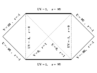
Figure 2: Carter-Penrose diagrams for the dilaton black holes with $0<a\leq 1$.

3 Euclidean dilaton black hole

Let us start with the Euclidean version of the BH. It is obtained from the metric (3) using the Wick rotation of the Killing time $t=i\tau$, the Euclidean time being periodic with the period $\beta=1/T_{\mathrm{B}H}=4\pi$.

$$ds^{2}=z(1-z)^{a-1}d\tau^{2}+{(1-z)^{a-3}\over z}~{}dz^{2},\hskip 28.45274pt0\leq\tau\leq 4\pi,\hskip 14.22636pt0\leq z\leq 1.$$ (4)

In the Euclidean case it is useful to rewrite the metric in another coordinate system $(\theta,\varphi)$

$$\cos(\theta)=1-2z,\hskip 28.45274pt\varphi={1\over 2}\tau.$$

in which it is explicitly conformal to a sphere $S^{2}$.

$$ds^{2}=\left({1+\cos\left(\theta\right)\over 2}\right)^{a-2}\left[d\theta^{2}+\sin(\theta)^{2}~{}d\varphi^{2}\right],\hskip 28.45274pt0\leq\theta\leq\pi,\hskip 14.22636pt0\leq\varphi\leq 2\pi.$$ (5)

The corresponding scalar curvature for this geometry is

$$R=a\left({1+\cos\theta\over 2}\right)^{2-a},\hskip 28.45274pt\sqrt{g}R=a\sin\theta$$

At the point $\theta=\pi$ we have to be more accurate. If $1<a<2$ and the point $\theta=\pi$ is not excluded from the manifold then there is a conical singularity at this point (see, e.g., the $a=3/2$ case right picture in figure 3) and one has to add $\delta$-like singular curvature term

$$R=\left({1+\cos\theta\over 2}\right)^{2-a}\left[a+(2-a)\delta\left({1+\cos\theta\over 2}\right)\right].$$

For compact manifolds the inclusion of conical singularity term guarantees the correct value of the topological invariant $\int d^{2}x\sqrt{g}R=8\pi$. Embeddings of these manifolds to a 3D flat space are depicted in figure (3). When $a=2$ the conical singularity disappears and we have the metric of a unit sphere, describing, obviously, an analytic continuation of the de Sitter space.

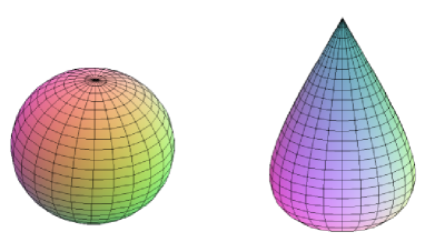
Figure 3: Embeddings of the Euclidean $a=2$ (on the left) and $a=3/2$ (on the right) geometries to a flat 3D space.

If $0<a\leq 1$ then the Euclidean manifolds have the topology of a disk (see figure 4) and conical singularities do not appear.

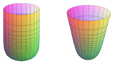
Figure 4: Embeddings of the Euclidean CGHS black hole (on the left, $a=1$) and a dilaton black hole with $a=1/2$ (on the right) to a flat 3D space.

4 Euclidean vacuum

Now let us consider quantum fields, $\phi$, which are non-minimally coupled to the scalar curvature on this background. The equation for free fields in 2D can always be written in the form

$$\left(\Box-\xi R\right)\phi=0$$

The Euclidean Green function is the solution of the equation

$$\left(\Box-\xi R\right)G_{E}(\theta,\varphi;\theta^{\prime},\varphi^{\prime})=-{\delta(\theta-\theta^{\prime})\delta(\varphi-\varphi^{\prime})\over\sqrt{g}}.$$ (6)

When quantum fields are assumed to be regular at “south pole” ($\theta=\pi$) it’s explicit form reads

$$\left[\partial_{\theta}\left(\sin\theta~{}\partial_{\theta}\right)+{1\over\sin\theta}\partial^{2}_{\varphi}-a\xi\sin\theta\right]G_{E}(\theta,\varphi;\theta^{\prime},\varphi^{\prime})=-\delta(\theta-\theta^{\prime})\delta(\varphi-\varphi^{\prime}).$$ (7)

A remarkable property of this Green function is that the parameter $a$ enters the equation only in the combination $a\xi$. If we put $a\xi=2\tilde{\xi}+m^{2}$ then this equation is identical to that of a massive non-conformal scalar field on the 2D sphere

$$\left(\Box-\tilde{\xi}R-m^{2}\right)G_{E}(\theta,\varphi;\theta^{\prime},\varphi^{\prime})\Big{|}_{{\cal M}=S^{2}}=-{\delta(\theta-\theta^{\prime})\delta(\varphi-\varphi^{\prime})\over\sqrt{g}}.$$

It means that in spite of the quite different geometries of the spacetimes in question non-minimal quantum fields do not distinguish between them after the rescaling of the constant $a\xi$.

The Green function for the non-minimal scalar field in the background of the Euclidean CGHS black hole $(a=1)$ has been found in [5] (see Eqs.(5.30)-(5.31)). In order to make more transparent the comparison of our results with the de Sitter case [2] and other dilaton black holes we define $a\xi=-\nu(\nu+1)$ or

$$\nu=-{1\over 2}+\sqrt{{1\over 4}-a~{}\xi}.$$ (8)

Then, for arbitrary $a>0$ in the metric (3) the Euclidean Green function can be written in terms of the Legendre function exactly as for CGHS black hole case (see [5])

$$G_{E}(X,X^{\prime})=-{1\over 4\sin(\pi\nu)}~{}P_{\nu}(-\lambda),$$ (9)

where

$$\lambda = (1-2z)(1-2z^{\prime})+4\sqrt{zz^{\prime}(1-z)(1-z^{\prime})}\cos\left({\tau-\tau^{\prime}\over 2}\right)$$ (10)

$$= \cos\theta\cos\theta^{\prime}+\sin\theta\sin\theta^{\prime}\cos(\varphi-\varphi^{\prime}).$$

The dependence on the geometry described by the constant $a$ comes only via the parameter $\nu$. $G_{E}(X,X^{\prime})$ is regular at “antipodal” points ($\lambda=-1$) and has a proper logarithmic divergence at coincident points ($\lambda\rightarrow 1$). Strictly speaking $\lambda=-1$ means that points are antipodal only in the 2D sphere case. But the coordinate dependence of Green functions for all other spaces is also encoded in the universal function $\lambda(X,X^{\prime})$ which in general is no longer a trivial function of the geodesic distance between points.

The mode expansion of the Green function can be written in the form

$$G_{E}(X,X^{\prime}) = -{1\over 4\sin(\pi\nu)}~{}\Big{[}~{}P_{\nu}(-1+2z^{<})~{}P_{\nu}(1-2z^{>})$$ (11)

$$+ 2\sum_{n=1}^{\infty}(-1)^{n}\cos\left({n(\tau-\tau^{\prime})\over 2}\right)~{}P^{~{}n}_{\nu}(-1+2z^{<})~{}P^{-n}_{\nu}(1-2z^{>})\Big{]}~{}.$$

After an analytical continuation to the Minkowskian signature this Green function gives the Feynmann propagator for quantum fields in the Euclidean vacuum state. The de Sitter Green function corresponds to $a=2$ and CGHS black hole case to $a=1$. Of course in the Minkowskian signature one can consider a set of different vacuum states and the Feynmann propagator depends on their choice. The Euclidean vacuum is only one of the possibilities. Moreover, if one wants to take into account interactions, there are additional constraints on a possible choice of the vacuum state. In order to get a meaningful perturbation theory the Feynmann propagator should satisfy the composition principle [2].

5 Composition principle

The variations of both the Euclidean Green function $G_{E}$ and the Feynmann propagator should satisfy the following rule

$$\delta G=G\delta\hat{F}G,$$

where

$$\hat{F}G=-\hat{1},\hskip 28.45274pt\Leftrightarrow\hskip 28.45274pt\sqrt{g}\hat{F}G(x,x^{\prime})=-\delta(x-x^{\prime}).$$

So, if we consider the following variation of the operator $\delta\hat{F}=-R\delta\xi$, then the Green functions must fulfill the identity

$${\partial}_{\xi}G(x,y)=-\int dx^{\prime}\sqrt{g(x^{\prime})}~{}G(x,x^{\prime})R(x^{\prime})G(x^{\prime},y)$$ (12)

In the case of a 2D unit sphere, which corresponds to $a=2$ and the scalar curvature $R=2$, this variational rule is equivalent to the composition principle

$${1\over 2}{\partial}_{\tilde{\xi}}G(x,y)={\partial}_{m^{2}}G(x,y)=-\int dx^{\prime}\sqrt{g(x^{\prime})}~{}G(x,x^{\prime})G(x^{\prime},y)$$ (13)

proposed by Polyakov as a property of Green functions necessary for the quantum state to be “eternal” [2]. The composition principle lies at the foundation of quantum field theory and its violation would be unacceptable for any quantum field theory which takes into account interactions.

In the case of a 2D Euclidean dilatonic black hole the Ricci scalar is not constant, but $\xi R\sqrt{g}\big{|}_{EBH}\leftrightarrow({2\tilde{\xi}+m^{2}})\sqrt{g}\big{|}_{S^{2}}$. Therefore, taking into account the coincidence of equations for Green functions in both spaces we see that the “eternity” condition (13) formally coincides with Eq.(12). For the Euclidean Green functions Eq.(9) this property Eq.(12) naturally follows from the property of the Legendre functions.

The Feynmann propagator can be obtained formally by analytic continuation from the Euclidean Green function.

$$G_{E}(X,X^{\prime})=-{1\over 4\sin(\pi\nu)}~{}P_{\nu}(-\lambda-i0)$$ (14)

This propagator corresponds to a particular choice of the vacuum state. In the case of the de Sitter spacetime it is known as the Bunch-Davies or Hartle-Hawking vacuum. Sometimes this state is also called the Euclidean vacuum. This is why we have kept here the subscript $E$ though it is defined for spacetimes with the Minkowskian signature.

Let us consider an example of 2D de Sitter spacetime. In global coordinates it has the form

$$ds^{2}=-d\tau^{2}+\cosh^{2}{\tau}d\tilde{\varphi}^{2},\hskip 28.45274pt-\infty<\tau<\infty,\hskip 28.45274pt0\leq\tilde{\varphi}\leq 2\pi,$$

and the de Sitter invariant quantity

$$\lambda=\cosh\tau\cosh\tau^{\prime}\cos(\tilde{\varphi}-\tilde{\varphi}^{\prime})-\sinh\tau\sinh\tau^{\prime},$$

is greater than $1$ for timelike separations and less then $1$ for spacelike separations. As a result of the different range of integration in the Eq.(13) the composition rule is violated for the Euclidean vacuum [2] since the Legendre function $P_{\nu}(-\lambda)$ blows up in the asymptotic $\lambda\rightarrow\infty$ and the integral over the spacetime diverges. The Euclidean vacuum is not the only de Sitter invariant vacuum. The Green functions for other de Sitter invariant vacuum states can be written as a linear combination of $P_{\nu}(\lambda+i0)$ and $Q_{\nu}(\lambda+i0)$. Here $i0$ is added to the argument of the Legendre functions in order to define the propagator on the cut $[-\infty,1]$ in the complex plane of $\lambda$. Polyakov proposed [2] that the Feynmann propagator which satisfies the composition principle for the de Sitter space is given by the formula

$$G_{Q}(X,X^{\prime}) = {1\over 2\pi}Q_{\nu}(\lambda+i0).$$ (15)

It corresponds to a different vacuum state and differs from the Euclidean vacuum propagator. The difference can be written explicitly

$$G_{Q}(X,X^{\prime}) = G_{E}(X,X^{\prime})+{{\mathrm{e}}^{-i\pi\nu}\over 4\sin(\pi\nu)}~{}P_{\nu}(\lambda+i0)$$ (16)

The Green function Eq.(15) decreases at $\lambda\rightarrow\infty$ and the integral in Eq.(13) converges provided ${\Re}(\nu)>-1/2$. $G_{Q}$ has a proper divergence at coincident points and there is also an extra divergence for antipodal points. Evidently, the corresponding quantum state belongs to the class of $\alpha-$vacua [6, 7, 8, 9, 10, 11]. In the de Sitter spacetime $G_{Q}$ is the only Feynmann propagator which respects the composition rule. Nevertheless, even this vacuum state is not stable and decays. This instability can be proved [2] using analytic properties of $Q_{\nu}(\lambda)$.

Though the generic spacetimes Eq.(1) do not respect the de Sitter symmetry, the Green functions still have the form Eq.(15) of the Feynmann propagators in the de Sitter spacetime. Therefore, the above discussion of their properties is applicable to all these spacetimes and one can conclude that Q-vacuum for dilaton black holes decays as well.

6 Bound states, quasinormal modes and spacetime instability

In static coordinates $(t,r)$ (see Eq.(3)) Fourier modes $\phi_{\omega}$ with fixed frequency $\omega$ satisfy the equation

$$\left[\partial_{r}(1-r^{2})\partial_{r}+\frac{4\omega^{2}}{1-r^{2}}-a\xi\right]\phi_{\omega}=0$$ (17)

The independent solutions of this equation are $P^{2i\omega}_{\nu}(r)$ and $Q^{2i\omega}_{\nu}(r)$. The Euclidean propagator $G_{E}$ is the sum of terms

$${\mathrm{e}}^{-i\omega(t-t^{\prime})}P^{2i\omega}_{\nu}(r)~{}P^{-2i\omega}_{\nu}(-r^{\prime})$$

with a prefactors proportional to the thermal occupation number $n(\omega)={1\over{\mathrm{e}}^{4\pi\omega}-1}$ corresponding to the inverse temperature $\beta=2\pi/\kappa=4\pi$. The $G_{Q}$ propagator is a similar sum of terms

$${\mathrm{e}}^{-i\omega(t-t^{\prime})}P^{2i\omega}_{\nu}(r)~{}Q^{-2i\omega}_{\nu}(r^{\prime})$$

Let us study an evolution of the modes with various boundary conditions. Any mode with a frequency $\omega$ is given by a linear combination of the Legendre functions $P^{2i\omega}_{\nu}(r)$ and $Q^{2i\omega}_{\nu}(r)$ or they can be equally well expressed in terms of hypergeometric functions (see, e.g., [5]). The frequency in these formulas can be taken as any complex number depending on the boundary conditions imposed on the modes. The solutions with real frequencies describe wavelike excitations. Complex frequencies are related to quasinormal modes while modes with pure imaginary frequencies appear to describe bound states. In the paper [5] it has been shown that for a CGHS black hole bound states appear when $\xi$ is negative. In this case perturbations grow exponentially with time and lead to a severe ”tachionic” instability of the black hole. It’s quite interesting that the unstable modes appear in the region outside the horizon, where the potential barrier has a minimum. Bound modes create fluxes of energy from this region to infinity and to the horizon and, because of the back reaction, eventually strongly deform the background geometry.

In our case the modes are determined by the same formula (4.7) from the paper [5], but $a\xi$ being substituted for $\xi$.

$$\omega_{n}={i\over 2}\left(\nu-n\right)={i\over 2}\left(\sqrt{{1\over 4}-a\xi}-{1\over 2}-n\right)$$ (18)

When $a\xi$ is negative and decreases further the number of bound states increases. A new bound state appears every time when $\nu=\sqrt{{1\over 4}-a\xi}-{1\over 2}$ reaches a new integer number value. This automatically leads to the conclusion that quantum fields with negative $a\xi$ cause ”tachionic” instability for all spacetimes described by the metrics Eq.(1) including the dilaton black holes and the de Sitter space.

The modes which are ingoing at the horizon $\sim{\mathrm{e}}^{-i\omega(t+x^{*})}$ and outgoing at infinity $\sim{\mathrm{e}}^{-i\omega(t-x^{*})}$ are called quasinormal modes (QNM). The parameters of QNMs can be easily determined from the position of poles in the complex $\omega$-plane of a transmission coefficient (see, e.g., Eq.(3.30) in [5])

$$|T_{\omega}|^{2}={\cosh(4\pi\omega)-1\over\cosh(4\pi\omega)+\cos\left(2\pi\sqrt{{1\over 4}-a\xi}\right)}$$ (19)

through the potential barrier. When the frequency is pure imaginary with positive imaginary part they describe bound states Eq.(18). The unstable behavior of 2D black holes against scalar perturbations discussed in [12] is directly related with the instability because of the bound states [5].

For other values of $a\xi$ the frequencies Eq.(18) may have both imaginary and real parts. If $a\xi>{1\over 4}$, then the quasinormal modes $\omega_{n}$ are

$$\omega_{n}={1\over 2}\sqrt{a\xi-{1\over 4}}-i~{}{1+2n\over 4}.$$ (20)

Here we see that the real part $\Re(\omega_{n})={1\over 2}\sqrt{a\xi-{1\over 4}}$ of the quasinormal modes does not depend on $n$ in accord with the high damping limit conjecture [13, 14] for QNMs. In pure de Sitter spacetime ($a=2,~{}2\xi=m^{2}$) quasinormal modes Eq.(18) correspond to those of 2D case in [15, 16].

7 Discussion

2D dilaton gravity models appear as effective gravity theories after a dimensional reduction from higher dimensions, in string theory, and in many other applications. The advantage of studying quantum fields in 2D spacetimes is that it is much easier to find exact solutions in this case, while reproducing qualitatively the same physical effects such as the Hawking radiation, thermodynamics etc.. Well known examples are CGHS model [1] and the de Sitter spacetime. In this paper we have found that these two models are related. Moreover they, in fact, have many more relatives. As for the non-conformal quantum fields on these backgrounds, they are exactly solvable for all members of this family and their physical properties are basically the same. The difference is encoded only in one real parameter $a$ Eq.(1), which marks the representative of the family.

For example, exact quasinormal modes are described by the common formulae Eqs.(18), (20). It is surprising because the geometries of these spacetimes are quite different. From this result one can see that there is no real part for quasinormal modes as soon as $\xi\leq{1\over 4a}$. When $\xi\geq{1\over 4a}$ a real part appears and it is the same for all $n$. The real part ${1\over 2}\sqrt{a\xi-{1\over 4}}$ can be any real number, while the Hawking temperature is the same for all these spacetimes. This observation can be considered as a counterexample to the conjecture, that the real part of highly damped QNMs is to be proportional to the logarithm of an integer number. This conjecture has been widely discussed in the literature in relation with the black holes quantization (see, e.g., review of the problem and references on the subject in the paper by R.G. Daghigh and G. Kunstatter [13]).

If scalar fields have negative coupling $\xi$ then bound modes arise outside the horizon of CGHS black hole [5]. This lead to classical instability of the system similar to tachionic one. The observed equivalence of CGHS black hole, de Sitter spacetime and other dilaton models leads to the conclusion that as soon as $a\xi<0$ bound modes appear for all these metrics along with the same destructive instabilities. For the positive non-minimal coupling quantum instabilities appear to arise similar to instabilities discussed by Polyakov [2] in application to the de Sitter. Their interpretation in the black hole case requires more detailed analysis and would be very interesting to examine.