The perfect magnetic conductor (PMC) Casimir piston
in $d\!+\!1$ dimensions

Perfect magnetic conductor (PMC) boundary conditions are dual to the more familiar perfect electric conductor (PEC) conditions and can be viewed as the electromagnetic analog of the boundary conditions in the bag model for hadrons in QCD. Recent advances and requirements in communication technologies have attracted great interest in PMC’s and Casimir experiments involving structures that approximate PMC’s may be carried out in the not too distant future. In this paper, we make a study of the zero-temperature PMC Casimir piston in $d\!+\!1$ dimensions. The PMC Casimir energy is explicitly evaluated by summing over $p+1$-dimensional Dirichlet energies where $p$ ranges from $2$ to $d$ inclusively. We derive two exact $d$-dimensional expressions for the Casimir force on the piston and find that the force is negative (attractive) in all dimensions. Both expressions are applied to the case of 2+1 and 3+1 dimensions. A spin-off from our work is a contribution to the PEC literature: we obtain a useful alternative expression for the PEC Casimir piston in 3+1 dimensions and also evaluate the Casimir force per unit area on an infinite strip, a geometry of experimental interest.

1 Introduction

Perfect magnetic conductor (PMC) boundary conditions are dual to the more familiar perfect electric conductor (PEC) conditions. In 3+1 dimensions, the electric field ${\bf E}$ and the magnetic field ${\bf B}$ are zero inside a PEC and the condition at the surface is ${\bf n\cdot B}=0$ and ${\bf n\times E}=0$ where n is the vector normal to the surface. The conditions for PMC’s is obtained via the dual transformations ${\bf E\to H}$ and ${\bf B\to-D}$ where ${\bf H}$ is the magnetic field strength and ${\bf D}$ the electric displacement. Inside a PMC, ${\bf D}$ and ${\bf H}$ are zero, and the condition at the surface becomes ${\bf n\cdot D}=0$ and ${\bf n\times H}=0$. PMC boundary conditions can be generalized to any dimension and are analogous to the boundary conditions in the bag model for hadrons in QCD (see next section).

A distinctive property of a PMC is that its surface reflects electromagnetic waves without phase change of the electric field, in contrast to the $\pi$ phase change from a PEC [1]. In the last few years there has been a great interest in structures which approximate PMC’s because of their usefulness to communication technologies, in particular low-profile antennas [1]. Casimir experiments involving structures which approximate PMC’s could therefore be carried out in the not too distant future. This would be an exciting development.

In this paper, we make a study of the zero-temperature PMC Casimir piston in a $d\!+\!1$ dimensional parallelepiped geometry. The PMC Casimir energy can be expressed as sums over Dirichlet energies of different dimensions and we perform this sum explicitly. We derive two different and exact expressions for the $d$-dimensional Casimir force on the piston. The second (alternative) expression is more useful than the first expression when the plate separation is larger than the dimension of the plates and vice-versa when the plate separation is smaller. The PMC Casimir force is negative (attractive) as in the PEC case (see refs. [4]-[8]), Dirichlet case [2, 3, 4, 8] and Neumann case [4, 8, 9]. The $d$-dimensional formulas (both expressions) are applied to the case of 2+1 and 3+1 dimensions and our results agree with previous Dirichlet and PEC results (see section 3). A spin-off from our work on PMC’s is a contribution to the PEC literature. We obtain a novel alternative expression for the 3+1 dimensional PEC Casimir piston and also calculate the Casimir force per unit area on an infinite strip, a case of experimental interest.

The piston geometry has attracted considerable attention since the original work of Cavalcanti [2] because it resolves the issue of surface divergences that often plague Casimir calculations [10] and moreover, includes the non-trivial effects of the exterior region. A Casimir piston contains an interior and an exterior region and Cavalcanti showed explicitly for the case of a massless scalar field in a 2+1 dimensional rectangular cavity that the surface terms of the interior and exterior regions canceled. He also showed that the Casimir force on the piston is always negative regardless of the ratios of the two sides of the rectangular region. This is in contrast to calculations that can yield positive Casimir forces in rectangular geometries when no exterior region is considered (see references in [11]).

The PEC Casimir piston at zero-temperature in a 3+1-dimensional square cavity was first studied in [4] and exact results were obtained for the Casimir force on the piston. It was also shown that the force was attractive. Expressions for arbitrary cross-section valid for small plate separation were also derived. Moreover, in that same work, the authors studied the Dirichlet and Neumann piston in 3+1 dimensions obtaining results for small plate separation (exact results were then obtained in [3, 8, 9]; see paragraph below). The PEC work was generalized further in [5] (see also [6, 7]) where exact results for arbitrary cross sections at zero and finite temperature were first obtained for arbitrary separation. The arbitrary cross-section results were applied to both rectangular and circular cross-sections and explicit expressions were obtained for these geometries. A positive feature of the Casimir expressions in [5] is that they are manifestly negative. Using an optical path technique, finite temperature results for the PEC rectangular piston with arbitrary separation were later obtained in a different form [8](arbitrary cross section results valid for small plate separation were also obtained). The physical meaning behind the various terms that contribute to the Casimir energy of a rectangular cavity was recently discussed as a three step process involving piston interactions [12]. It is worth noting that Casimir forces in a piston geometry can be repulsive (positive) under various conditions. This was discussed in [13, 14].

Besides the usual electromagnetic field, there is also good reason to consider massless scalar fields in Casimir calculations. As discussed in [4, 8], the PEC Casimir energy can be obtained from the Dirichlet and Neumann energy. Moreover, Casimir results for massless scalar fields have been shown to have direct application to physical systems such as Bose-Einstein condensates [15, 16, 17]. Higher-dimensional scalar field Casimir calculations have also appeared in 6D supergravity theories [18] and recently, the Casimir force on a piston with extra compactified dimensions has been investigated [19]. As already mentioned above, scalar fields in the 3+1 dimensional piston scenario were first studied in [4] and approximate results valid for small plate separation were obtained. Exact results for the zero-temperature 3+1 dimensional Dirichlet piston with rectangular cross-section was then obtained in [3] via a multidimensional cut-off technique [20]. Exact zero and finite temperature results for the 3+1 Neumann and Dirichlet piston with rectangular cross sections were then obtained in [8]. Shortly thereafter, using a different technique, two different expressions for the zero-temperature 3+1 Neumann piston with rectangular cross section were obtained in [9]. The zero-temperature Dirichlet and Neumann Casimir piston for parallelepiped geometries was solved exactly in arbitrary dimensions in [9]. The $d$-dimensional formulas were applied to the 2+1 (and 3+1) dimensional Neumann piston bringing a completion to Cavalcanti’s original work in 2+1 dimensions [2].

2 PMC Casimir piston in d+1-dimensions

The PMC boundary conditions ${\bf n\cdot E}\!=\!0$ and ${\bf n\times B}\!=\!0$ can be expressed as $\eta^{\mu}F_{\mu\nu}=0$ where $F_{\mu\nu}\equiv\partial_{\mu}A_{\nu}-\partial_{\nu}A_{\mu}$ is the electromagnetic field tensor and $\eta^{\mu}$ is a spacelike vector normal to the surface. This is analogous to the boundary conditions in the bag model for hadrons in QCD. We choose the gauge condition $A_{0}\!=\!0$ and $\partial^{i}A_{i}\!=\!0$. The PMC condition $\eta^{\mu}F_{\mu\nu}\!=\!0$ together with the gauge condition applies to any dimension. The mode decomposition for a parallelepiped geometry in $d\!+\!1$ dimensions with sides of lengths $L_{i}$ where $i$ runs from $1$ to $d$ inclusively is given by [21]:

$$A_{i}=c_{i}\sin(k_{i}\,x_{i})\prod_{\begin{subarray}{c}j=1\\ j\neq i\end{subarray}}^{d}\cos(k_{j}\,x_{j})\,e^{-i\omega t}$$ (2.1)

where $k_{p}=n_{p}\,\pi/L_{p}$, $n_{p}\geq 0\in N$ and $\omega\!=\!(k_{p}\,k^{p})^{1/2}$ where $p$ runs from $1$ to $d$ inclusively. The PMC Casimir energy can be decomposed into sums of Dirichlet energies of different dimensions. When all $n_{i}$’s are non-zero, there are $d$ modes but the gauge condition reduces this by $1$ yielding $d\!-\!1$ independent modes. When one of the $n_{i}$’s is zero, there are $d\!-\!2$ independent modes. In general, there are $d\!-\!j$ independent modes when $j\!-\!1$ $n_{i}$’s are zero (where $j$ runs from $1$ to $d\!-\!1$ inclusively). Each of those modes has the energy of a scalar field in $d\!-\!j\!+\!1$ dimensions obeying Dirichlet boundary conditions. One must sum over all distinct sets of $d\!-\!j\!+\!1$ lengths chosen among the $d$ lengths $L_{1},L_{2},..,L_{d}$. The Casimir energy $E$ for PMC boundary conditions in a $d\!+\!1$ dimensional parallelepiped geometry with sides of length $L_{1},L_{2},..,L_{d}$ can therefore be expressed as sums over Dirichlet(D) Casimir energies $E_{D}$ (in units where $\hbar\!=\!c\!=\!1$) [21]:

$$E=\sum_{j=1}^{d-1}\,(d-j)\,\,\xi^{d}_{\,i_{1},..,i_{d-j+1}}\,E_{D_{\,i_{1},..,i_{d-j+1}}}\,.$$ (2.2)

There is an implicit summation over the integers $i_{j}$ in (2.2). The ordered symbol $\xi^{d}_{\,i_{1},..,i_{p}}$, originally introduced in [3], is defined as

$$\xi^{\,d}_{\,i_{1},..,i_{p}}=\begin{cases}1&\,\,\mbox{if}\,\,i_{1}\!<\!i_{2}\!<\!\ldots\!<i_{p}\,;\,1\leq i_{p}\leq d\\ 0&\,\,\mbox{otherwise}\,\,.\end{cases}$$ (2.3)

For $p=0$, $\xi^{d}_{\,i_{1},..,i_{p}}$ is defined to be unity. The ordered symbol ensures that the implicit sum over the $i_{j}$’s is over all distinct sets $\{i_{1},\ldots,i_{p}\}$, where the $i_{j}$’s are integers that can run from $1$ to $d$ inclusively under the constraint that $i_{1}\!<\!i_{2}\!<\!\cdots\!<i_{p}$. The superscript $d$ specifies the maximum value of $i_{p}$. For example, if $p=2$ and $d=3$ then $\xi^{\,d}_{\,i_{1},..,i_{p}}=\xi^{\,3}_{\,i_{1},i_{2}}$ and the non-zero terms are $\xi_{\,1,2}$ , $\xi_{\,1,3}$ and $\xi_{\,2,3}$. This means the summation is over $\{i_{1},i_{2}\}=(1,2),(1,3)$ and $(2,3)$ so that $\xi^{\,3}_{\,i_{1},i_{2}}\,E_{i_{1}\,i_{2}}=E_{12}+E_{13}+E_{23}$. The expression for the $d$-dimensional Dirichlet Casimir energy was previously obtained and is given by [3, 9]

$$E_{D_{1,2,..,d}}=\dfrac{\pi}{2^{d+1}}\sum_{p=0}^{d-1}(-1)^{d+p}\,\,\xi^{\,d-1}_{\,k_{1},..,k_{p}}\,\dfrac{L_{k_{1}}\ldots L_{k_{p}}}{(L_{d})^{p+1}}\big{(}Q_{p}+R_{D_{p}}\big{)}\,$$ (2.4)

where $Q_{p}$ is a function of $p$ and a product of gamma and Riemann zeta functions:

$$Q_{p}=\Gamma(\tfrac{p+2}{2})\,\pi^{\frac{-p-4}{2}}\,\zeta(p+2)\,.$$ (2.5)

$R_{D_{p}}$ can be thought of as a remainder and is an infinite sum over modified Bessel functions that converges rapidly

$$R_{D_{p}}=\sum_{n=1}^{\infty}\,\sideset{}{{}^{\prime}}{\sum}_{\begin{subarray}{c}\ell_{i}=-\infty\\ i=1,\ldots,p\end{subarray}}^{\infty}\dfrac{2\,\,n^{\frac{p+1}{2}}}{\pi}\,\dfrac{\,K_{\frac{p+1}{2}}\big{(}\,2\pi\,n\,\sqrt{(\ell_{1}\frac{L_{k_{1}}}{L_{d}})^{2}+\cdots+(\ell_{p}\,\frac{L_{k_{p}}}{L_{d}})^{2}}\,\,\,\big{)}}{\left[(\ell_{1}\frac{L_{k_{1}}}{L_{d}})^{2}+\cdots+(\ell_{p}\frac{L_{k_{p}}}{L_{d}})^{2}\right]^{\tfrac{p+1}{4}}}\,.$$ (2.6)

The prime on the sum in (2.6) means that the case when all $\ell$’s are simultaneously zero ($\ell_{1}\!=\!\ell_{2}\!=\!\ldots\!=\!\ell_{p}\!=\!0$) is to be excluded. There is an implicit summation over the $k_{i}$’s via the ordered symbol $\xi_{\,k_{1},..,k_{p}}$ defined in (2.3). Unlike $Q_{p}$, $R_{D_{p}}$ does not depend only on $p$ but is also a function of the ratios of lengths i.e. $R_{D_{p}}=R_{D_{p}}(L_{k_{1}}/L_{d},\ldots,L_{k_{p}}/L_{d})$. Therefore, the implicit summation over the $k_{i}$’s applies also to $R_{D_{p}}$. For $p=0$, $R_{D_{p}}$ is defined to be zero and $\xi_{\,k_{1},..,k_{p}}$ and $L_{k_{p}}$ are defined to be unity so that $\xi^{\,d-1}_{\,k_{1},..,k_{p}}\,(L_{k_{1}}\ldots L_{k_{p}})/(L_{d})^{p+1}=1/L_{d}$ for $p=0$.

The piston divides the volume into two regions: region I (inside) and region II (outside). In region I, the $d$ sides are of length $a_{1},a_{2},..,a_{d-1},a$ where $a$ is the plate separation. The $d$ sides are labeled in the following fashion: $L_{1}\!=\!a_{1}$, $L_{2}\!=\!a_{2}$, $L_{d-1}\!=\!a_{d-1}$ and $L_{d}\!=\!a$. The Casimir force depends on the derivative with respect to $a$ of the Casimir energy and therefore only those terms which contain $L_{d}\!=\!a$ need to be included. For the Casimir energy $E_{D_{\,i_{1},..,i_{d-j+1}}}$ appearing in (2.2), the length $L_{d}$ occurs when $i_{d-j+1}=d$ (recall that $i_{1}\!<\!i_{2}\!<\!..\!<\!i_{d-j+1}$). Therefore

$$\xi^{d}_{\,i_{1},..,i_{d-j+1}}\,E_{D_{\,i_{1},..,i_{d-j+1}}}=\xi^{d-1}_{\,i_{1},..,i_{d-j}}\,E_{D_{\,i_{1},..,i_{d-j},d}}\,.$$ (2.7)

The formula for $E_{D_{\,i_{1},..,i_{d-j},d}}$ is obtained by replacing $d$ by $d\!-\!j\!+\!1$ and $L_{k_{1}}$ by $L_{i_{k_{1}}}$, $L_{k_{p}}$ by $L_{i_{k_{p}}}$ and $L_{d}$ by $L_{i_{d-j+1}}\!=\!L_{d}$ in (2.4):

$$E_{D_{\,i_{1},..,i_{d-j},d}}=\dfrac{\pi}{2^{(d-j+2)}}\sum_{p=0}^{d-j}(-1)^{d+p-j+1}\,\,\xi^{\,d-j}_{\,k_{1},..,k_{p}}\,\dfrac{L_{i_{k_{1}}}\ldots L_{i_{k_{p}}}}{(L_{d})^{p+1}}\big{(}Q_{p}+R_{p}\big{)}\,$$ (2.8)

where $R_{p}$ is equal to $R_{D_{p}}$ with $L_{k_{1}}$ replaced by $L_{i_{k_{1}}}$, $L_{k_{p}}$ by $L_{i_{k_{p}}}$ and $L_{d}$ by $L_{i_{d-j+1}}\!=\!L_{d}$.

To evaluate $\xi^{d-1}_{\,i_{1},..,i_{d-j}}\,E_{D_{\,i_{1},..,i_{d-j},d}}$ we need to determine $\xi^{d-1}_{\,i_{1},..,i_{d-j}}\xi^{\,d-j}_{\,k_{1},..,k_{p}}\,L_{i_{k_{1}}}\ldots L_{i_{k_{p}}}$. The number of distinct sets $(i_{1},..,i_{d-j})$ that can be generated by $\xi^{d-1}_{\,i_{1},..,i_{d-j}}$ is the binomial coefficient $\Bigl{(}\genfrac{}{}{0.0pt}{}{d-1}{d-j}\Bigr{)}$. The number of those sets that contain a particular set $(i_{k_{1}},..,i_{k_{p}})$ is simply $\Bigl{(}\genfrac{}{}{0.0pt}{}{d-1-p}{d-j-p}\Bigr{)}$. We therefore obtain

$$\xi^{d-1}_{\,i_{1},..,i_{d-j}}\xi^{\,d-j}_{\,k_{1},..,k_{p}}\,L_{i_{k_{1}}}\ldots L_{i_{k_{p}}}=\Bigl{(}\genfrac{}{}{0.0pt}{}{d\!-\!1\!-\!p}{d\!-\!j\!-\!p}\Bigr{)}\,\xi^{\,d-1}_{\,k_{1},..,k_{p}}\,L_{k_{1}}\ldots L_{k_{p}}\,.$$ (2.9)

As an illustration consider the case $d\!=\!5$, $p\!=\!2$ and $j\!=\!2$. Evaluating the left hand side of (2.9) yields

$$\begin{split}&\xi^{d-1}_{\,i_{1},..,i_{d-j}}\xi^{\,d-j}_{\,k_{1},..,k_{p}}\,L_{i_{k_{1}}}\ldots L_{i_{k_{p}}}=\xi^{4}_{\,i_{1},i_{2},i_{3}}\,\xi^{\,3}_{\,k_{1},k_{2}}\,L_{i_{k_{1}}}L_{i_{k_{2}}}=\xi^{4}_{\,i_{1},i_{2},i_{3}}(\xi^{\,3}_{1,2}L_{i_{1}}L_{i_{2}}+\xi^{3}_{1,3}\,L_{i_{1}}L_{i_{3}}+\xi^{3}_{2,3}\,L_{i_{2}}L_{i_{3}})\\ &=\xi^{4}_{\,i_{1},i_{2},i_{3}}(L_{i_{1}}L_{i_{2}}+L_{i_{1}}L_{i_{3}}+L_{i_{2}}L_{i_{3}})=\xi^{4}_{\,1,2,3}(L_{1}L_{2}+L_{1}L_{3}+L_{2}L_{3})+\xi^{4}_{\,1,2,4}(L_{1}L_{2}+L_{1}L_{4}+L_{2}L_{4})\\ &+\xi^{4}_{\,1,3,4}(L_{1}L_{3}+L_{1}L_{4}+L_{3}L_{4})+\xi^{4}_{\,2,3,4}(L_{2}L_{3}+L_{2}L_{4}+L_{3}L_{4})\\ &=2\,(L_{1}L_{2}+L_{1}L_{3}+L_{1}L_{4}+L_{2}L_{3}+L_{2}L_{4}+L_{3}L_{4})\,.\end{split}$$ (2.10)

The right hand side of (2.9) yields

$$\Bigl{(}\genfrac{}{}{0.0pt}{}{d\!-\!1\!-\!p}{d\!-\!j\!-\!p}\Bigr{)}\,\xi^{\,d-1}_{\,k_{1},..,k_{p}}\,L_{k_{1}}\ldots L_{k_{p}}=\Bigl{(}\genfrac{}{}{0.0pt}{}{2}{1}\Bigr{)}\xi^{\,4}_{\,k_{1},k_{2}}\,L_{k_{1}}L_{k_{2}}=2\,(L_{1}L_{2}+L_{1}L_{3}+L_{1}L_{4}+L_{2}L_{3}+L_{2}L_{4}+L_{3}L_{4})$$ (2.11)

which is equal to the result in (2.10).

The Casimir energy in region I, $E_{I}$, is obtained by substituting (2.7) into (2.2) and then using formula (2.8) and the equality (2.9):

$$\begin{split}E_{I}&=\sum_{j=1}^{d-1}\sum_{p=0}^{d-j}(-1)^{d+p-j+1}\dfrac{\pi}{2^{(d-j+2)}}(d-j)\Bigl{(}\genfrac{}{}{0.0pt}{}{d\!-\!1\!-\!p}{d\!-\!j\!-\!p}\Bigr{)}\,\xi^{\,d-1}_{\,k_{1},..,k_{p}}\,\dfrac{L_{k_{1}}\ldots L_{k_{p}}}{(L_{d})^{p+1}}\big{(}Q_{p}+R_{p}\big{)}\\ &=\sum_{p=0}^{d-1}\sum_{j=1}^{d-p}(-1)^{d+p-j+1}\dfrac{\pi}{2^{(d-j+2)}}(d-j)\Bigl{(}\genfrac{}{}{0.0pt}{}{d\!-\!1\!-\!p}{d\!-\!j\!-\!p}\Bigr{)}\,\xi^{\,d-1}_{\,k_{1},..,k_{p}}\,\dfrac{a_{k_{1}}\ldots a_{k_{p}}}{a^{p+1}}\big{(}Q_{p}+R_{I_{p}}\big{)}\,.\end{split}$$ (2.12)

Note that we have rearranged the double sum, replaced $L_{d}$ by the plate separation $a$ and $L_{k_{i}}$ by $a_{k_{i}}$. The sum over $j$ can be readily evaluated and yields

$$\sum_{j=1}^{d-p}(-1)^{d+p-j+1}\dfrac{d-j}{2^{(d-j+2)}}\Bigl{(}\genfrac{}{}{0.0pt}{}{d\!-\!1\!-\!p}{d\!-\!j\!-\!p}\Bigr{)}=\dfrac{(d\!-\!1\!-\!2\,p)}{2^{d+1}}\,.$$ (2.13)

We finally obtain for region I

$$E_{I}=\dfrac{\pi}{2^{d+1}}\sum_{p=0}^{d-1}\,(d\!-\!1\!-\!2\,p)\,\,\xi^{\,d-1}_{\,k_{1},..,k_{p}}\,\dfrac{a_{k_{1}}\ldots a_{k_{p}}}{a^{p+1}}\,\big{(}Q_{p}+R_{I_{p}}\big{)}$$ (2.14)

where $Q_{p}$ is given by (2.5) and $R_{I_{p}}$ is obtained from $R_{D_{p}}$ by replacing $L_{k_{i}}$ by $a_{k_{i}}$ and $L_{d}$ by the plate separation $a$ i.e.

$$R_{I_{p}}=\sum_{n=1}^{\infty}\,\sideset{}{{}^{\prime}}{\sum}_{\begin{subarray}{c}\ell_{i}=-\infty\\ i=1,\ldots,p\end{subarray}}^{\infty}\dfrac{2\,\,n^{\frac{p+1}{2}}}{\pi}\,\dfrac{\,K_{\frac{p+1}{2}}\big{(}\,2\pi\,n\,\sqrt{(\ell_{1}\frac{a_{k_{1}}}{a})^{2}+\cdots+(\ell_{p}\,\frac{a_{k_{p}}}{a})^{2}}\,\,\,\big{)}}{\left[(\ell_{1}\frac{a_{k_{1}}}{a})^{2}+\cdots+(\ell_{p}\frac{a_{k_{p}}}{a})^{2}\right]^{\tfrac{p+1}{4}}}\,.$$ (2.15)

We now evaluate the PMC Casimir energy in region II, $E_{II}$. In region II, the $d$ lengths are $s-a$, $a_{1},a_{2},..,a_{d-1}$ (i.e. the same lengths as in region I except that $a$ is replaced by $s\!-\!a$). We label the lengths in region II as $L_{1}=s\!-\!a$, $L_{2}=a_{1}$, $L_{3}=a_{2}$ and $L_{d}=a_{d-1}$. The Casimir force is obtained by taking the derivative with respect to $a$ so that only terms that contain $L_{1}$ need to be included in the Casimir energy. We therefore set $i_{1}=1$ in (2.2) which yields

$$E_{I\!I}=\sum_{j=1}^{d-1}\,(d-j)\,\,\xi^{d}_{\,1,i_{2},i_{3},..,i_{d-j+1}}\,E_{D_{\,1,i_{2},i_{3},..,i_{d-j+1}}}\,$$ (2.16)

where the Dirichlet expression is given by (2.4):

$$E_{D_{\,1,i_{2},i_{3}..,i_{d-j+1}}}=\dfrac{\pi}{2^{(d-j+2)}}\sum_{p=1}^{d-j}(-1)^{d+p-j+1}\,\,\xi^{\,d-j}_{\,1,k_{2},k_{3},..,k_{p}}\,\dfrac{L_{1}\,L_{i_{k_{2}}}\ldots L_{i_{k_{p}}}}{(L_{i_{d-j+1}})^{p+1}}\big{(}Q_{p}+R_{{I\!I}_{p}}\big{)}\,.$$ (2.17)

$R_{{II}_{p}}$ is obtained from $R_{D_{p}}$ eq. (2.6) with $L_{k_{1}}$ replaced by $L_{1}\!=\!s\!-\!a$, $L_{k_{p}}$ by $L_{i_{k_{p}}}$ and $L_{d}$ by $L_{i_{d-j+1}}$. Substituting (2.17) into (2.16) yields:

$$E_{I\!I}=\sum_{j=1}^{d-1}\,\sum_{p=1}^{d-j}(-1)^{d+p-j+1}\,\dfrac{\pi}{2^{(d-j+2)}}\,(d-j)\,\xi^{d}_{\,1,i_{2},i_{3},..,i_{d-j+1}}\,\xi^{\,d-j}_{\,1,k_{2},k_{3},..,k_{p}}\,\dfrac{L_{1}\,L_{i_{k_{2}}}\ldots L_{i_{k_{p}}}}{(L_{i_{d-j+1}})^{p+1}}\big{(}Q_{p}+R_{{I\!I}_{p}}\big{)}$$ (2.18)

In $\xi^{d}_{\,1,i_{2},i_{3},..,i_{d-j+1}}$ the value of $i_{d-j+1}$ ranges from $d\!-\!j\!+\!1$ to $d$ inclusively. We can therefore replace $i_{d-j+1}$ with $d-q$ and sum $q$ from $0$ to $j-1$ yielding

$$\begin{split}\xi^{d}_{\,1,i_{2},i_{3},..,i_{d-j+1}}\,\xi^{\,d-j}_{\,1,k_{2},k_{3},..,k_{p}}\,\dfrac{L_{1}\,L_{i_{k_{2}}}\ldots L_{i_{k_{p}}}}{(L_{i_{d-j+1}})^{p+1}}&=\sum_{q=0}^{j-1}\xi^{d-q-1}_{\,1,i_{2},i_{3},..,i_{d-j},d-q}\,\xi^{\,d-j}_{\,1,k_{2},k_{3},..,k_{p}}\,\dfrac{L_{1}\,L_{i_{k_{2}}}\ldots L_{i_{k_{p}}}}{(L_{d-q})^{p+1}}\\ &=\sum_{q=0}^{j-1}\Bigl{(}\genfrac{}{}{0.0pt}{}{d\!-\!q\!-\!1\!-\!p}{d\!-\!j\!-\!p}\Bigr{)}\,\xi^{\,d-q-1}_{\,1,k_{2},k_{3},..,k_{p}}\,\dfrac{L_{1}\,L_{k_{2}}\ldots L_{k_{p}}}{(L_{d-q})^{p+1}}\,\end{split}$$ (2.19)

where the binomial coefficient follows from the same reasoning given above (2.9).

Substituting the above into (2.18) yields

$$\begin{split}E_{I\!I}\!&=\!\sum_{j=1}^{d-1}\sum_{p=1}^{d-j}\sum_{q=0}^{j-1}(-1)^{d+p-j+1}\,\dfrac{\pi\,(d-j)}{2^{(d-j+2)}}\,\Bigl{(}\genfrac{}{}{0.0pt}{}{d\!-\!q\!-\!1\!-\!p}{d\!-\!j\!-\!p}\Bigr{)}\,\xi^{\,d-q-1}_{\,1,k_{2},k_{3},..,k_{p}}\,\dfrac{L_{1}\,L_{k_{2}}\ldots L_{k_{p}}}{(L_{d-q})^{p+1}}\big{(}Q_{p}+R_{{I\!I}_{p}}\big{)}\\ &=\sum_{p=1}^{d-1}\sum_{q=0}^{d-p-1}\sum_{j=q+1}^{d-p}(-1)^{d+p-j+1}\,\dfrac{\pi\,(d-j)}{2^{(d-j+2)}}\,\Bigl{(}\genfrac{}{}{0.0pt}{}{d\!-\!q\!-\!1\!-\!p}{d\!-\!j\!-\!p}\Bigr{)}\,\xi^{\,d-q-1}_{\,1,k_{2},k_{3},..,k_{p}}\,\dfrac{(s-a)\,a_{k_{2}-1}\ldots a_{k_{p}-1}}{(a_{d-q-1})^{p+1}}\big{(}Q_{p}+R_{{I\!I}_{p}}\big{)}\,\end{split}$$ (2.20)

where the triple sum has been rearranged into an equivalent form and the lengths corresponding to the $L_{i}$’s was substituted. The sum over $j$ yields

$$\sum_{j=q+1}^{d-p}(-1)^{d+p-j+1}\,\dfrac{(d-j)}{2^{(d-j+2)}}\,\Bigl{(}\genfrac{}{}{0.0pt}{}{d\!-\!q\!-\!1\!-\!p}{d\!-\!j\!-\!p}\Bigr{)}\,=\dfrac{(d\!-\!1\!-\!2\,p\!-\!q)}{2^{d-q+1}}\,$$ (2.21)

and we finally obtain the PMC Casimir energy $E_{I\!I}$ for region II:

$$E_{I\!I}=\sum_{p=1}^{d-1}\,\,\sum_{q=0}^{d-p-1}\dfrac{\pi\,(d\!-\!1\!-\!2p\!-\!q)}{2^{d-q+1}}\,\,\xi^{\,d-q-1}_{\,1,k_{2},k_{3},..,k_{p}}\,\dfrac{(s-a)\,a_{k_{2}-1}\ldots a_{k_{p}-1}}{(a_{d-q-1})^{p+1}}\big{(}Q_{p}+R_{{I\!I}_{p}}\big{)}\,$$ (2.22)

where $Q_{p}$ is again given by (2.5) and $R_{I\!I_{p}}$ is obtained from eq.(2.6) with $L_{k_{1}}$ replaced by $L_{1}\!=\!s\!-\!a$, $L_{k_{p}}$ by $a_{k_{p}-1}$ and $L_{d}$ by $a_{d-q-1}$ i.e.

$$R_{I\!I_{p}}=\sum_{n=1}^{\infty}\,\sideset{}{{}^{\prime}}{\sum}_{\begin{subarray}{c}\ell_{i}=-\infty\\ i=1,\ldots,p\end{subarray}}^{\infty}\dfrac{2\,\,n^{\frac{p+1}{2}}}{\pi}\,\dfrac{\,K_{\frac{p+1}{2}}\big{(}\,2\pi\,n\,\sqrt{(\ell_{1}\frac{s-a}{a_{d-q-1}})^{2}+\cdots+(\ell_{p}\,\frac{a_{k_{p}-1}}{a_{d-q-1}})^{2}}\,\,\,\big{)}}{\left[(\ell_{1}\frac{s-a}{a_{d-q-1}})^{2}+\cdots+(\ell_{p}\frac{a_{k_{p}-1}}{a_{d-q-1}})^{2}\right]^{\tfrac{p+1}{4}}}\,.$$ (2.23)

2.1 PMC Casimir force expressions in d+1 dimensions

The Casimir force is obtained by taking the negative derivative with respect to the plate separation $a$ of the Casimir energy. In region I the Casimir energy is given by (2.14) together with (2.5) and (2.15). The Casimir force in region I, $F_{I}$ is given by

$$\begin{split}F_{I}&=-\dfrac{\partial\,E_{I}}{\partial\,a}\\ &=\dfrac{\pi}{2^{d+1}}\sum_{p=0}^{d-1}\,(d\!-\!1\!-\!2p)\,(p+1)\,\,\xi^{\,d-1}_{\,k_{1},..,k_{p}}\,\dfrac{a_{k_{1}}\ldots a_{k_{p}}}{a^{p+2}}\,\,\Gamma(\tfrac{p+2}{2})\,\,\pi^{\frac{-p-4}{2}}\,\,\zeta(p+2)\,-\,\dfrac{\partial\,R_{I}}{\partial\,a}\end{split}$$ (2.24)

where

$$\begin{split}\dfrac{\partial\,R_{I}}{\partial\,a}&=\dfrac{\partial}{\partial\,a}\Bigg{\{}\dfrac{\pi}{2^{d+1}}\sum_{p=1}^{d-1}\,(d\!-\!1\!-\!2p)\,\,\xi^{\,d-1}_{\,k_{1},..,k_{p}}\dfrac{\,a_{k_{1}}\ldots a_{k_{p}}}{a^{p+1}}\,R_{I_{p}}\Bigg{\}}\\ &=\dfrac{\pi}{2^{d-1}}\sum_{p=1}^{d-1}\,\sum_{n=1}^{\infty}\,\sideset{}{{}^{\prime}}{\sum}_{\begin{subarray}{c}\ell_{i}=-\infty\\ i=1,\ldots,p\end{subarray}}^{\infty}(d\!-\!1\!-\!2p)\,\,\xi^{\,d-1}_{\,k_{1},..,k_{p}}\,a_{k_{1}}\ldots a_{k_{p}}\,n^{\frac{p+3}{2}}\,\dfrac{\,K_{\frac{p-1}{2}}\big{(}\,\frac{2\pi\,n}{a}\,\sqrt{(\ell_{1}\,a_{k_{1}})^{2}+\cdots+(\ell_{p}\,a_{k_{p}})^{2}}\,\,\,\big{)}}{a^{\frac{p+5}{2}}\,\left[(\ell_{1}\,a_{k_{1}})^{2}+\cdots+(\ell_{p}\,a_{k_{p}})^{2}\right]^{\tfrac{p-1}{4}}}\,.\end{split}$$ (2.25)

The Casimir energy in region II is given by (2.22) together with (2.5) and (2.23). We are interested in the case when the outside region $II$ is infinite i.e. $s\to\infty$. The Casimir force in region $II$ is then given by

$$\begin{split}F_{I\!I}&=-\lim_{s\to\infty}\dfrac{\partial\,E_{I\!I}}{\partial\,a}\\ &=\sum_{p=1}^{d-1}\,\,\sum_{q=0}^{d-p-1}\dfrac{\pi\,(d\!-\!1\!-\!2p\!-\!q)}{2^{d-q+1}}\,\,\xi^{\,d-q-1}_{\,1,k_{2},k_{3},..,k_{p}}\,\dfrac{a_{k_{2}-1}\ldots a_{k_{p}-1}}{(a_{d-q-1})^{p+1}}\\ &\qquad\qquad\qquad\qquad\qquad\qquad\Big{\{}\Gamma(\tfrac{p+2}{2})\,\,\pi^{\frac{-p-4}{2}}\,\,\zeta(p+2)\,-\lim_{s\to\infty}\,\dfrac{\partial\,}{\partial\,a}\big{\{}(s-a)\,R_{{I\!I}_{p}}\big{\}}\Big{\}}\\ &=\sum_{p=1}^{d-1}\,\,\sum_{q=0}^{d-p-1}\dfrac{\pi\,(d\!-\!1\!-\!2p\!-\!q)}{2^{d-q+1}}\,\,\xi^{\,d-q-1}_{\,1,k_{2},k_{3},..,k_{p}}\,\dfrac{a_{k_{2}-1}\ldots a_{k_{p}-1}}{(a_{d-q-1})^{p+1}}\,\Big{\{}\Gamma(\tfrac{p+2}{2})\,\,\pi^{\frac{-p-4}{2}}\,\,\zeta(p+2)\,+R_{{I\!I}_{p}}(\ell_{1}\!=\!0)\Big{\}}\end{split}$$ (2.26)

where $R_{{I\!I}_{p}}(\ell_{1}\!=\!0)$ means $R_{{I\!I}_{p}}$ evaluated with $\ell_{1}\!=\!0$:

$$R_{I\!I_{p}}(\ell_{1}\!=\!0)=\sum_{n=1}^{\infty}\,\sideset{}{{}^{\prime}}{\sum}_{\begin{subarray}{c}\ell_{i}=-\infty\\ i=2,\ldots,p\end{subarray}}^{\infty}\dfrac{2\,\,n^{\frac{p+1}{2}}}{\pi}\,\dfrac{\,K_{\frac{p+1}{2}}\big{(}\,2\pi\,n\,\sqrt{(\ell_{2}\frac{a_{k_{2}-1}}{a_{d-q-1}})^{2}+\cdots+(\ell_{p}\,\frac{a_{k_{p}-1}}{a_{d-q-1}})^{2}}\,\,\,\big{)}}{\left[(\ell_{2}\frac{a_{k_{2}-1}}{a_{d-q-1}})^{2}+\cdots+(\ell_{p}\frac{a_{k_{p}-1}}{a_{d-q-1}})^{2}\right]^{\tfrac{p+1}{4}}}\,.$$ (2.27)

The Casimir force $F_{\!P\!M\!C}$ on the piston with perfect magnetic conductor boundary conditions is finally obtained by adding $F_{I}$ and $F_{I\!I}$:

$$\begin{split}F_{\!P\!M\!C}&=\dfrac{\pi}{2^{d+1}}\sum_{p=0}^{d-1}\,(d\!-\!1\!-\!2p)\,(p+1)\,\,\xi^{\,d-1}_{\,k_{1},..,k_{p}}\,\dfrac{a_{k_{1}}\ldots a_{k_{p}}}{a^{p+2}}\,\,\Gamma(\tfrac{p+2}{2})\,\,\pi^{\frac{-p-4}{2}}\,\,\zeta(p+2)\,-\,\dfrac{\partial\,R_{I}}{\partial\,a}\\ &\qquad\qquad+\sum_{p=1}^{d-1}\,\,\sum_{q=0}^{d-p-1}\dfrac{\pi\,(d\!-\!1\!-\!2p\!-\!q)}{2^{d-q+1}}\,\,\xi^{\,d-q-1}_{\,1,k_{2},k_{3},..,k_{p}}\,\dfrac{a_{k_{2}-1}\ldots a_{k_{p}-1}}{(a_{d-q-1})^{p+1}}\,\\ &\qquad\qquad\qquad\qquad\qquad\qquad\qquad\qquad\qquad\Big{\{}\Gamma(\tfrac{p+2}{2})\,\,\pi^{\frac{-p-4}{2}}\,\,\zeta(p+2)\,+R_{{I\!I}_{p}}(\ell_{1}\!=\!0)\Big{\}}\,\end{split}$$ (2.28)

where $\partial\,R_{I}/\partial\,a$ is given by (2.25) and $R_{{I\!I}_{p}}(\ell_{1}\!=\!0)$ by (2.27). The PMC Casimir force in any spatial dimension $d$ and for arbitrary lengths of the sides of the parallelepiped can be obtained via equation (2.28) together with (2.25) and (2.27). The force is automatically negative (attractive) because it is obtained from a sum over Dirichlet Casimir piston forces which are negative.

We now discuss the rate of convergence of (2.28). Note that (2.28) contains two different kinds of terms: a finite sum over analytical terms and infinite sums over modified Bessel functions. The analytical terms contain inverse powers of the plate separation $a$ (i.e. $1/a^{p+2}$) multiplied by gamma and Riemann zeta functions. A finite sum of those terms is trivial to evaluate and there are no convergence issues. The next term, $\partial R_{I}/\partial a$ given by (2.25), contains infinite sums over modified Bessel functions. The ratios of lengths in the argument of the modified Bessel functions have the plate separation $a$ in the denominator. If $a$ is the smallest length, the modified Bessel functions are tiny and the sum converges exponentially fast (only a few terms need to be summed in (2.25) to reach convergence). However, if the plate separation $a$ is the largest length (e.g. square plates with sides of 1 micron separated by 10 microns), the modified Bessel functions can be large and converge slowly. In the large $a$ limit where $a_{k_{i}}/a<\!<1$, a large number of terms would need to be summed in (2.25) to achieve convergence. Simply put, when $a$ is large, it is not computationally efficient to use (2.28) to evaluate the Casimir force.

By using the invariance of the Casimir energy under permutation of lengths, it is possible to derive an alternative expression for the PMC Casimir force $F_{P\!M\!C}^{alt}$ that yields the same force as (2.28) but converges exponentially fast when the plate separation $a$ is the largest length. This expression is derived in appendix A and is given by (A.6) together with (A.7). In (A.7), the plate separation $a$ appears in the ${\it numerator}$ in the argument of the modified Bessel functions so that the infinite sums converge exponentially fast when $a$ is the largest length. Computationally it is better to use the alternative expression (A.6) instead of the above expression (2.28) to calculate the PMC Casimir force when the plate separation $a$ is the largest length and vice versa if $a$ is the smallest length. The main results of this paper are the two different expressions for the PMC Casimir force on the piston: equations (2.28) and (A.6).

3 Applications: the 2+1 and 3+1 dimensional PMC Casimir piston

As an illustration of how to apply the $d\!+\!1$-dimensional PMC Casimir formula (2.28) or the alternative expression (A.6) we consider 2+1 and 3+1 dimensions. The case of 2+1 dimensions is the simplest non-trivial case where equations (2.28) and (A.6) can be applied. From (2.2), we see that in two spatial dimensions, the PMC Casimir energy is equivalent to the Dirichlet energy. In three spatial dimensions (and only in three), the PMC Casimir energy is equal to the PEC Casimir energy. This can be seen most transparently in the transverse electric (TE) and transverse magnetic (TM) decomposition that exists in 3+1 dimensions. The PEC Casimir energy in 3+1 is half the sum over all modes of the eigenfrequencies $\omega_{TE}$ and $\omega_{TM}$ (see [5] for a recent application of the TE/TM decomposition in a piston geometry of arbitrary cross section). The eigenfrequencies in the PMC case are obtained by simply switching $\omega_{TE}$ for $\omega_{TM}$ and vice-versa leaving the sum $\omega_{TE}\!+\!\omega_{TM}$ unchanged. A strong confirmation of our $d$-dimensional technique and PMC formulas is that our 2+1 and 3+1 dimensional results are in agreement with previous Dirichlet and PEC results respectively. An important spin-off from our work is that we obtain an alternative expression for the PEC Casimir piston in 3+1 dimensions and also obtain the Casimir force per unit area for the special case of an infinite strip.

3.1 2+1 dimensions

In $2\!+\!1$ dimensions we use $d=2$ in (2.28). The two lengths are $a_{1}=b$ and the plate separation $a$. We evaluate the three terms in (2.28) separately. The first term is

$$\begin{split}\dfrac{\pi}{8}\sum_{p=0}^{1}\,(1-2p)(p+1)\xi^{\,1}_{\,k_{1},..,k_{p}}\,\dfrac{a_{k_{1}}\ldots a_{k_{p}}}{a^{p+2}}\,\,\Gamma(\tfrac{p+2}{2})\,\,\pi^{\frac{-p-4}{2}}\,\,\zeta(p+2)=\dfrac{\pi}{48\,a^{2}}-\dfrac{\zeta(3)\,b}{8\pi a^{3}}\,.\end{split}$$ (3.29)

The second term is evaluated via eq.(2.25) with $d=2$:

$$-\,\dfrac{\partial\,R_{I}}{\partial\,a}=\dfrac{\pi\,b}{a^{3}}\,\sum_{n=1}^{\infty}\,\sum_{\ell=1}^{\infty}\,n^{2}\,K_{0}\Big{(}\,\frac{2\pi\,n\,\ell\,b}{a}\Big{)}\,.$$ (3.30)

The third term yields (only the $p\!=\!1$, $q\!=\!0$ case needs to be evaluated):

$$\begin{split}&\dfrac{\pi\,(-1)}{2^{3}}\,\,\dfrac{1}{(a_{1})^{p+1}}\,\Big{\{}\Gamma(\tfrac{3}{2})\,\,\pi^{\frac{-5}{2}}\,\,\zeta(3)\,+R_{{I\!I}_{p}}(\ell_{1}\!=\!0)\Big{\}}\\ &=-\dfrac{\zeta(3)}{16\pi\,b^{2}}\,\end{split}$$ (3.31)

where $R_{{I\!I}_{p}}(\ell_{1}\!=\!0)$ is zero for $p=1$ (it starts at $p=2$). The PMC Casimir force on the piston in $2+1$ dimensions is given by summing all three terms:

$$F_{\!P\!M\!C}=-\dfrac{\zeta(3)\,b}{8\pi a^{3}}+\dfrac{\pi}{48\,a^{2}}+\dfrac{\pi\,b}{a^{3}}\,\sum_{n=1}^{\infty}\,\sum_{\ell=1}^{\infty}\,n^{2}\,K_{0}\Big{(}\,\frac{2\pi\,n\,\ell\,b}{a}\Big{)}-\dfrac{\zeta(3)}{16\pi\,b^{2}}\,.$$ (3.32)

In the limit of infinite parallel lines, i.e. $b\!\to\!\infty$, the force per unit length tends to $-\zeta(3)/8\pi a^{3}$.

We now calculate the Casimir force using the alternative expression (A.6) together with (A.7). For $d=2$, we only need to evaluate the term $(p\!=\!1,q\!=\!0)$ in (A.6):

$$F_{PMC}^{alt}=\dfrac{\pi}{8\,b^{2}}\dfrac{\partial\,}{\partial\,a}\Big{\{}a\,\sum_{n=1}^{\infty}\sum_{\ell=1}^{\infty}\dfrac{4}{\pi}\dfrac{n\,b}{\ell\,a}K_{1}\big{(}\frac{2\,\pi\,n\,\ell\,a}{b}\big{)}\Big{\}}=\dfrac{1}{2\,b}\sum_{n=1}^{\infty}\sum_{\ell=1}^{\infty}\dfrac{n}{\ell}\,\dfrac{\partial\,}{\partial\,a}K_{1}\big{(}\frac{2\,\pi\,n\,\ell\,a}{b}\big{)}\,.$$ (3.33)

Eqs. (3.32) and (3.33) are both in agreement with those obtained by Cavalcanti [2] for Dirichlet boundary conditions in $2\!+\!1$ dimensions and this provides an independent confirmation of our general PMC formulas (2.28) and (A.6).

3.2 3+1 dimensions

In $3+1$ dimensions we set $d=3$ in (2.28). The three lengths are $a_{1}=c$, $a_{2}=b$ and the plate separation $a$. Again we evaluate the three terms in (2.28) separately. The first term yields

$$\begin{split}\dfrac{\pi}{16}\sum_{p=0}^{2}\,(2-2p)(p+1)\xi^{\,2}_{\,k_{1},..,k_{p}}\,\dfrac{a_{k_{1}}\ldots a_{k_{p}}}{a^{p+2}}\,\,\Gamma(\tfrac{p+2}{2})\,\,\pi^{\frac{-p-4}{2}}\,\,\zeta(p+2)=\dfrac{\pi}{48\,a^{2}}-\dfrac{3\,b\,c\,\zeta(4)}{8\pi^{2}a^{4}}\,.\end{split}$$ (3.34)

The second term is given by

$$\begin{split}-\dfrac{\partial\,R_{I}}{\partial\,a}&=-\dfrac{\pi}{4}\sum_{p=1}^{2}\,\sum_{n=1}^{\infty}\,\sideset{}{{}^{\prime}}{\sum}_{\begin{subarray}{c}\ell_{i}=-\infty\\ i=1,\ldots,p\end{subarray}}^{\infty}(2-\!2p)\,\,\xi^{\,2}_{\,k_{1},..,k_{p}}\,a_{k_{1}}\ldots a_{k_{p}}\,n^{\frac{p+3}{2}}\,\dfrac{\,K_{\frac{p-1}{2}}\big{(}\,\frac{2\pi\,n}{a}\,\sqrt{(\ell_{1}\,a_{k_{1}})^{2}+\cdots+(\ell_{p}\,a_{k_{p}})^{2}}\,\,\,\big{)}}{a^{\frac{p+5}{2}}\,\left[(\ell_{1}\,a_{k_{1}})^{2}+\cdots+(\ell_{p}\,a_{k_{p}})^{2}\right]^{\tfrac{p-1}{4}}}\,\\ &=\dfrac{\pi\,b\,c}{2\,a^{7/2}}\,\sum_{n=1}^{\infty}\,\sideset{}{{}^{\prime}}{\sum}_{\begin{subarray}{c}\ell_{1},\ell_{2}=-\infty\\ \end{subarray}}^{\infty}n^{\frac{5}{2}}\,\dfrac{\,K_{\frac{1}{2}}\big{(}\,\frac{2\pi\,n}{a}\,\sqrt{(\ell_{1}\,c)^{2}+(\ell_{2}\,b)^{2}}\,\big{)}}{\,\left[(\ell_{1}\,c)^{2}+(\ell_{2}\,b)^{2}\right]^{\tfrac{1}{4}}}\end{split}$$ (3.35)

and the third term yields

$$\begin{split}&\sum_{p=1}^{2}\,\,\sum_{q=0}^{2-p}\dfrac{\pi\,(2-\!2p\!-\!q)}{2^{4-q}}\,\,\xi^{\,2-q}_{\,1,k_{2},k_{3},..,k_{p}}\,\dfrac{a_{k_{2}-1}\ldots a_{k_{p}-1}}{(a_{{}_{2\!-q}})^{p+1}}\Big{\{}\Gamma(\tfrac{p+2}{2})\,\,\pi^{\frac{-p-4}{2}}\,\,\zeta(p+2)\,+R_{{I\!I}_{p}}(\ell_{1}\!=\!0)\Big{\}}\\ &=-\dfrac{\zeta(3)}{16\,\pi c^{2}}-\dfrac{\zeta(4)\,c}{8\pi^{2}b^{3}}-\dfrac{1}{2\,c^{1/2}}\,\sum_{n=1}^{\infty}\,\sum_{\ell=1}^{\infty}\,\Big{(}\dfrac{n}{\ell\,b}\Big{)}^{3/2}\,K_{3/2}\Big{(}\,\frac{2\pi\,n\,\ell\,c}{b}\Big{)}\,.\end{split}$$ (3.36)

The PMC Casimir force in $3+1$ dimensions is obtained by summing all three terms i.e.

$$\begin{split}F_{\!P\!M\!C}&=\dfrac{\pi}{48\,a^{2}}-\dfrac{3\,\zeta(4)\,b\,c}{8\pi^{2}a^{4}}+\dfrac{\pi\,b\,c}{2\,a^{7/2}}\,\sum_{n=1}^{\infty}\,\sideset{}{{}^{\prime}}{\sum}_{\begin{subarray}{c}\ell_{1},\ell_{2}=-\infty\\ \end{subarray}}^{\infty}n^{\frac{5}{2}}\,\dfrac{\,K_{\frac{1}{2}}\big{(}\,\frac{2\pi\,n}{a}\,\sqrt{(\ell_{1}\,c)^{2}+(\ell_{2}\,b)^{2}}\,\big{)}}{\,\left[(\ell_{1}\,c)^{2}+(\ell_{2}\,b)^{2}\right]^{\tfrac{1}{4}}}\\ &-\dfrac{\zeta(3)}{16\,\pi c^{2}}-\dfrac{\zeta(4)\,c}{8\pi^{2}b^{3}}-\dfrac{1}{2\,c^{1/2}}\,\sum_{n=1}^{\infty}\,\sum_{\ell=1}^{\infty}\,\Big{(}\dfrac{n}{\ell\,b}\Big{)}^{3/2}\,K_{3/2}\Big{(}\,\frac{2\pi\,n\,\ell\,c}{b}\Big{)}\,.\end{split}$$ (3.37)

Though expressed in a different form, equation (3.37) is in numerical agreement with previous PEC results in 3+1 dimensions refs.[4]-[8]. This provides another independent confirmation of our $d$-dimensional equations.

To obtain the alternative expression for the Casimir force, we substitute $d=3$ in (A.6):

$$\begin{split}F_{\!P\!M\!C}^{alt}&=-\sum_{p=1}^{2}\,\,\sum_{q=0}^{2-p}\dfrac{\pi\,(2\!-\!2p\!-\!q)}{2^{4-q}}\,\,\xi^{\,2-q}_{\,1,k_{2},k_{3},..,k_{p}}\,\dfrac{a_{k_{2}-1}\ldots a_{k_{p}-1}}{(a_{2-q})^{p+1}}\dfrac{\partial\,}{\partial\,a}\big{\{}a\,R_{I_{p}}^{alt}(\ell_{1}\!\neq\!0)\big{\}}\\ &=\dfrac{1}{2\,c}\,\sum_{n=1}^{\infty}\sum_{\ell=1}^{\infty}\dfrac{n}{\ell}\dfrac{\partial\,}{\partial\,a}K_{1}\big{(}\frac{2\,\pi\,n\,\ell\,a}{c}\big{)}\\ &\qquad\qquad+\,\dfrac{\partial\,}{\partial\,a}\Bigg{\{}\dfrac{a\,c}{2}\sum_{n=1}^{\infty}\,\sum_{\ell_{1}=1}^{\infty}\sum_{\begin{subarray}{c}\ell_{2}=-\infty\\ \end{subarray}}^{\infty}\Big{(}\dfrac{n}{b}\Big{)}^{3/2}\,\dfrac{\,K_{\frac{3}{2}}\big{(}\,\frac{2\pi\,n}{b}\,\sqrt{(\ell_{1}\,a)^{2}+(\ell_{2}\,c)^{2}}\,\big{)}}{\left[(\ell_{1}\,a)^{2}+(\ell_{2}\,c)^{2}\right]^{\tfrac{3}{4}}}\Bigg{\}}\,.\end{split}$$ (3.38)

The alternative expression (3.38) yields the same value as the original expression (3.37) but converges much faster if $a$ is larger than $b$ and $c$. Note that (3.38) is also an alternative expression for the PEC Casimir piston in 3+1 dimensions. A spin-off from our work is therefore a novel expression for the PEC piston that is highly useful (converges fast) when $a$ is larger than $b$ and $c$.

3.2.1 Infinite strip

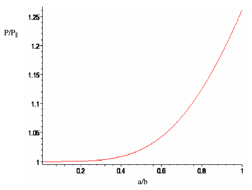
Figure 1: Casimir pressure on infinite strip versus $a/b$ (in units of $P_{||}$).

In this section we consider the special case of an infinite strip where one side of the plates is of finite length and the other side is infinitely long (yielding translation invariance along that direction). An accurate measurement of the Casimir force between parallel metallic surfaces was performed only a few years ago [23]. The infinite strip, being closely related in geometry, should therefore be of experimental interest. The 3+1 dimensional Casimir force given by eq. (3.37) is invariant under exchange of the two sides $b$ and $c$ and without loss of generality we take $b$ to be finite and let $c\to\infty$. In this limit, the term containing $K_{3/2}$ in (3.37) is zero and the term containing $K_{1/2}$ is zero except when $\ell_{1}$ equals zero. This yields a Casimir force per unit area (or pressure) of

$$P\equiv\lim_{c\to\infty}\,\dfrac{F}{b\,c}=-\dfrac{3\,\zeta(4)}{8\pi^{2}a^{4}}-\dfrac{\zeta(4)}{8\pi^{2}b^{4}}+\dfrac{\pi}{a^{7/2}}\,\sum_{n=1}^{\infty}\,\sum_{\ell=1}^{\infty}\,\,n^{\frac{5}{2}}\,\dfrac{\,K_{\frac{1}{2}}\big{(}\,\frac{2\pi\,n\,\ell\,b}{a}\big{)}}{\sqrt{\ell\,b}}\,.$$ (3.39)

After performing the sum over $\ell$ the above expression simplifies to

$$P=-\dfrac{3\,\zeta(4)}{8\pi^{2}a^{4}}-\dfrac{\zeta(4)}{8\pi^{2}b^{4}}-\dfrac{\pi}{2\,b\,a^{3}}\,\sum_{n=1}^{\infty}n^{2}\,\ln(1-e^{-2\,\pi\,n\,b\,/a})\,.$$ (3.40)

The first term represents the force per unit area between parallel plates i.e.

$$P_{||}=-\dfrac{3\,\zeta(4)}{8\pi^{2}\,a^{4}}\,.$$ (3.41)

The pressure $P$ expressed in units of $P_{||}$ reduces to the expression

$$\dfrac{P}{P_{||}}=1+\dfrac{1}{3}\bigg{(}\dfrac{a}{b}\bigg{)}^{4}+\dfrac{120}{\pi}\bigg{(}\dfrac{a}{b}\bigg{)}\,\sum_{n=1}^{\infty}n^{2}\,\ln(1-e^{-2\,\pi\,n\,b\,/a})\,.$$ (3.42)

We plot $P/P_{||}$ as a function of $a/b$ in Fig. 1. The Casimir pressure on the strip is greater than or equal to one and increases as $a/b$ increases, reaching a value that is $26\%$ higher than the parallel plate case when $b=a$.

4 Summary and discussion

In this paper we obtain two exact $d$-dimensional expressions for the PMC Casimir piston namely equations (2.28) and (A.6). We showed that the application of these formulas to 2+1 and 3+1 dimensions is in agreement with previous Dirichlet and PEC piston results. Moreover, as a spin-off, we obtain an alternative expression for the 3+1 dimensional PEC Casimir piston which is useful when the plate separation is larger than the dimension of the plates. We also calculated the Casimir force per unit area for the special case of an infinite strip, a geometry of experimental interest. We showed that the Casimir pressure on the strip is $26\%$ stronger compared to the pressure on parallel plates when the side $b$ of the strip equals the plate separation $a$.

The important role that Casimir energies can play when extra dimensions are present has recently been highlighted in [24]. It was argued that in a brane world scenario with toroidal extra dimensions, Casimir energies under certain conditions could stabilize the extra dimensions, allow three dimensions to grow large and provide an effective dark energy in the large dimensions. Higher-dimensional Casimir formulas derived in previous works were used and this illustrates the relevance of such results to investigations in different branches of Physics.

Driven in large part by communication technologies, the last four to five years have seen a great interest in structures which approximate PMC’s [1]. Casimir experiments involving such structures may therefore be possible in the not too distant future. In practice, experiments would yield different results between PEC and PMC pistons because one is comparing metals with finite electric conductivity to approximate PMC’s with finite magnetic conductivity. In PEC’s, we know that finite electric conductivity corrections can contribute on the order of 10 to 20 % of the net Casimir force for parallel plates separated by approximately $1\mu m$ [11]. It would therefore be worthwhile to calculate the effects of finite magnetic conductivity on PMC Casimir energies first in a parallel plate scenario and then a piston scenario. This is work for the future.

Appendix A Alternative expressions for the $d+1$-dimensional PMC Casimir piston

We can develop an alternative formula for the PMC Casimir force by simply labeling the $d$ lengths $L_{1},L_{2},..,L_{d}$ in region I differently while keeping the same labeling for region II. This will not alter the Casimir energy in region I because it is invariant under permutation of lengths. In our previous derivation leading to the $F_{\!P\!M\!C\!}$, eq. (2.28), we labeled the $d$ lengths in region I in the following fashion: $L_{1}=a_{1},L_{2}=a_{2},...,L_{d-1}=a_{d-1}$ and $L_{d}=a$ where $a$ is the plate separation. We now label them $L_{1}=a,L_{2}=a_{1},...,L_{d}=a_{d-1}$. Note that this is the same labeling we had for region $I\!I$ in our original derivation except that now $L_{1}$ is $a$ instead of $s-a$. This means that our alternative expression for the Casimir energy in region I, $E_{I}^{alt}$, can be obtained from the formula for $E_{I\!I}$ ((2.22) together with (2.23)) by replacing $s-a$ by $a$. This yields

$$E_{I}^{alt}=\sum_{p=1}^{d-1}\,\,\sum_{q=0}^{d-p-1}\dfrac{\pi\,(d\!-\!1\!-\!2p\!-\!q)}{2^{d-q+1}}\,\,\xi^{\,d-q-1}_{\,1,k_{2},k_{3},..,k_{p}}\,\dfrac{a\,a_{k_{2}-1}\ldots a_{k_{p}-1}}{(a_{d-q-1})^{p+1}}\big{(}Q_{p}+R_{{I}_{p}}^{alt}\big{)}\,$$ (A.1)

where $Q_{p}$ is given by (2.5) and $R_{I_{p}}^{alt}$ is obtained from (2.23) with $s\!-\!a$ replaced by $a$ i.e.

$$R_{I_{p}}^{alt}=\sum_{n=1}^{\infty}\,\sideset{}{{}^{\prime}}{\sum}_{\begin{subarray}{c}\ell_{i}=-\infty\\ i=1,\ldots,p\end{subarray}}^{\infty}\dfrac{2\,\,n^{\frac{p+1}{2}}}{\pi}\,\dfrac{\,K_{\frac{p+1}{2}}\big{(}\,2\pi\,n\,\sqrt{(\ell_{1}\frac{a}{a_{d-q-1}})^{2}+\cdots+(\ell_{p}\,\frac{a_{k_{p}-1}}{a_{d-q-1}})^{2}}\,\,\,\big{)}}{\left[(\ell_{1}\frac{a}{a_{d-q-1}})^{2}+\cdots+(\ell_{p}\frac{a_{k_{p}-1}}{a_{d-q-1}})^{2}\right]^{\tfrac{p+1}{4}}}\,.$$ (A.2)

The alternative expression for the Casimir force in region I is

$$\begin{split}F_{I}^{alt}&=-\dfrac{\partial\,E_{I}^{alt}}{\partial\,a}\\ &=-\sum_{p=1}^{d-1}\,\,\sum_{q=0}^{d-p-1}\dfrac{\pi\,(d\!-\!1\!-\!2p\!-\!q)}{2^{d-q+1}}\,\,\xi^{\,d-q-1}_{\,1,k_{2},k_{3},..,k_{p}}\,\dfrac{a_{k_{2}-1}\ldots a_{k_{p}-1}}{(a_{d-q-1})^{p+1}}\\ &\qquad\qquad\qquad\qquad\qquad\qquad\Big{\{}\Gamma(\tfrac{p+2}{2})\,\,\pi^{\frac{-p-4}{2}}\,\,\zeta(p+2)\,+\dfrac{\partial\,}{\partial\,a}\big{(}a\,R_{I_{p}}^{alt}\big{)}\Big{\}}\,.\end{split}$$ (A.3)

The expression for the Casimir force in region $I\!I$ is the same as before i.e. $F_{I\!I}$ given by eq.(2.26):

$$\begin{split}F_{I\!I}&=\sum_{p=1}^{d-1}\,\,\sum_{q=0}^{d-p-1}\dfrac{\pi\,(d\!-\!1\!-\!2p\!-\!q)}{2^{d-q+1}}\,\,\xi^{\,d-q-1}_{\,1,k_{2},k_{3},..,k_{p}}\,\dfrac{a_{k_{2}-1}\ldots a_{k_{p}-1}}{(a_{d-q-1})^{p+1}}\,\\ &\qquad\qquad\qquad\qquad\qquad\qquad\qquad\qquad\qquad\qquad\qquad\Big{\{}\Gamma(\tfrac{p+2}{2})\,\,\pi^{\frac{-p-4}{2}}\,\,\zeta(p+2)\,+R_{{I\!I}_{p}}(\ell_{1}\!=\!0)\Big{\}}\end{split}$$ (A.4)

where $R_{{I\!I}_{p}}(\ell_{1}\!=\!0)$ is given by (2.27). The alternative expression for the Casimir force on the piston, $F_{\!P\!M\!C}^{alt}$ is obtained by adding $F_{I}^{alt}$ and $F_{I\!I}$. Note that the first term in the curly brackets (the term with the Riemann zeta function) of $F_{I}^{alt}$ and $F_{I\!I}$ are identical except that one is the negative of the other. They therefore cancel out. Note also that the $\ell_{1}=0$ part of the second term in the curly brackets of $F_{I}^{alt}$ cancels out with the second term in $F_{I\!I}$ since

$$-\dfrac{\partial\,}{\partial\,a}\big{\{}a\,R_{I_{p}}^{alt}(\ell_{1}\!=\!0)\big{\}}=-R_{I_{p}}^{alt}(\ell_{1}\!=\!0)=-R_{{I\!I}_{p}}(\ell_{1}\!=\!0)\,.$$ (A.5)

The alternative expression for the PMC Casimir force reduces to

$$F_{\!P\!M\!C}^{alt}=F_{I}^{alt}+F_{I\!I}=-\sum_{p=1}^{d-1}\,\,\sum_{q=0}^{d-p-1}\dfrac{\pi\,(d\!-\!1\!-\!2p\!-\!q)}{2^{d-q+1}}\,\,\xi^{\,d-q-1}_{\,1,k_{2},k_{3},..,k_{p}}\,\dfrac{a_{k_{2}-1}\ldots a_{k_{p}-1}}{(a_{d-q-1})^{p+1}}\dfrac{\partial\,}{\partial\,a}\big{\{}a\,R_{I_{p}}^{alt}(\ell_{1}\!\neq\!0)\big{\}}$$ (A.6)

where $R_{I_{p}}^{alt}(\ell_{1}\!\neq\!0)$ is (A.2) evaluated without including $\ell_{1}\!=\!0$ i.e.

$$R_{I_{p}}^{alt}(\ell_{1}\!\neq\!0)=\sum_{n=1}^{\infty}\,\sum_{\ell_{1}=1}^{\infty}\sum_{\begin{subarray}{c}\ell_{i}=-\infty\\ i=2,\ldots,p\end{subarray}}^{\infty}\dfrac{4\,\,n^{\frac{p+1}{2}}}{\pi}\,\dfrac{\,K_{\frac{p+1}{2}}\big{(}\,2\pi\,n\,\sqrt{(\ell_{1}\frac{a}{a_{d-q-1}})^{2}+\cdots+(\ell_{p}\,\frac{a_{k_{p}-1}}{a_{d-q-1}})^{2}}\,\,\,\big{)}}{\left[(\ell_{1}\frac{a}{a_{d-q-1}})^{2}+\cdots+(\ell_{p}\frac{a_{k_{p}-1}}{a_{d-q-1}})^{2}\right]^{\tfrac{p+1}{4}}}\,.$$ (A.7)

In contrast to (A.2), there is no longer a prime on the sum over $\ell_{i}$ and it starts at $i\!=\!2$.

References

- [1] J. R. Sohn, K. Y. Kim, H.-S. Tae and H. J. Lee, PIER 61, 27 (2006); Y. Zhang, J. von Hagen and W. Wiesbeck, Microw. Opt. Technol. Lett. 35, 172 (2002); J. McVay, N. Engheta and A. Hoorfar, IEEE Microw. Wire. Comp. Lett. 14, 130 (2004); A. P. Feresidis, S. Wang and J. C. Vardaxoglou, IEEE Trans. Antennas Propag. 53, 209 (2005); F. Yang and Y. Rahmat-Samii, IEEE Trans. Antennas Propag. 51, 2691 (2003).
- [2] R. M. Cavalcanti, Phys. Rev. D 69, 065015 (2004).
- [3] A. Edery, Phys. Rev. D 75, 105012 (2007) hep-th/0610173.
- [4] M.P. Hertzberg, R.L. Jaffe, M. Kardar and A. Scardicchio, Phys. Rev. Lett 95, 250402 (2005).
- [5] V. Marachevsky, Phys. Rev. D 75, 085019 (2007) hep-th/0703158.
- [6] V. Marachevsky, hep-th/0609116.
- [7] V. Marachevsky, hep-th/0512221.
- [8] M.P. Hertzberg, R.L. Jaffe, M. Kardar and A. Scardicchio, Phys. Rev. D 76, 045016 (2007) [arXiv:0705.0139].
- [9] A. Edery and I. MacDonald, JHEP 09 (2007) 005 [arXiv:0708.0392].
- [10] N. Graham, R. Jaffe, V. Khemani, M. Quandt, O. Schroeder and H. Weigel, Nucl. Phys. B 677, 379 (2004).
- [11] M. Bordag, U. Mohideen and V.M. Mostepanenko, Phys.Rept. 353, 1 (2001). 4083 (2001).
- [12] V. Marachevsky, J. Phys. A: Math. Theor. 41 (2008) 164007 [arXiv:0710.4130].
- [13] G. Barton, Phys. Rev. D 73, 065018 (2006).
- [14] S.A. Fulling, L. Kaplan and J.H. Wilson, Phys. Rev. A 76, 012118 (2007) [arXiv:0703248].
- [15] A. Edery, J. Stat. Mech. P06007 (2006) [hep-th/0510238].
- [16] D.C. Roberts and Y. Pomeau, Phys. Rev. Lett. 95, 145303 (2005).
- [17] C. Barcel, S. Liberati and M. Visser, Class. Quantum Grav. 18, 3595 (2001).
- [18] D.M. Ghilencea, D. Hoover, C.P. Burgess and F. Quevedo, JHEP 0509, 050 (2005) [hep-th/0506164].
- [19] H. Cheng, [arXiv:0801.2810].
- [20] A. Edery, J. Phys. A: Math. Gen. 39, 685 (2006).
- [21] J. Ambjørn and S. Wolfram, Ann. Phys. (N.Y.) 147, 1 (1983).
- [22] H. G. Casimir, Proc. Kon. N. Akad. Wet. 51, 793 (1948).
- [23] G. Bressi, G. Carugno, R. Onofrio and G. Ruoso, Phys. Rev. Lett. 88, 041804 (2002).
- [24] B.R. Greene and J. Levin, JHEP 096 (2007) 0711 [arXiv:0707.1062].