Production of electroweak gauge bosons in off-shell
gluon-gluon fusion

Abstract

We study the production of electroweak gauge bosons at high energies in the framework of $k_{T}$-factorization QCD approach. The amplitude for production of a single $W^{\pm}$ or $Z^{0}$ boson associated with quark pair in the fusion of two off-shell gluons is calculated. Contributions from the valence quarks are calculated using the quark-gluon interaction and quark-antiquark annihilation QCD subprocesses. The total and differential cross sections (as a function of the transverse momentum and rapidity) are presented and the ratio of cross sections for $W^{\pm}$ and $Z^{0}$ boson production is investigated. The conservative error analysis is performed. In the numerical calculations two different sets of unintegrated gluon distributions in the proton are used: the one obtained from Ciafaloni-Catani-Fiorani-Marchesini evolution equation and the other from Kimber-Martin-Ryskin prescription. Theoretical results are compared with experimental data taken by the D$\oslash$ and CDF collaborations at the Tevatron. We demonstrate the importance of the quark component in parton evolution in description of the experimental data. This component is very significant also at the LHC energies.

PACS number(s): 12.38.Bx, 12.15.Ji

1 Introduction

The theoretical and experimental studying the vector ($W^{\pm}$ and $Z^{0}$) boson production at high energies provide information about the nature of both the underlying electroweak interaction and the effects of Quantum Chromodynamics (QCD). In many respects these processes have become one of most important ”standard candles” in experimental high energy physics [1–9]. At the Tevatron, measurements of $W^{\pm}$ and $Z^{0}$ inclusive cross sections are routinely used to validate detector and trigger perfomance and stability. Data from gauge boson production also provide bounds on parametrizations used to describe the non-perturbative regime of QCD processes. At the LHC, such measurements can serve as a useful tool to determine the integrated luminosity and can also be used to normalize measurements of other production cross sections (for example, cross section of $W+n$-jets or diboson production). Additionally, studying of inclusive vector boson production is necessary starting point for investigations of Higgs or top quark production where many signatures can include these bosons.

At leading order (LO) of QCD, $W^{\pm}$ and $Z^{0}$ bosons are produced via quark-antiquark annihilation. Beyond the LO Born process, vector boson can also be produced by $q+g$ interactions, so both the quark and gluon distribution functions of the proton play an important role. Theoretical calculations of the $W^{\pm}$ and $Z^{0}$ production cross sections have been carried out at next-to-leading order (NLO) and next-to-next-to-leading order (NNLO) [10–14] of QCD. The NLO cross section is $\sim 25$% larger than the Born-level cross section, and the NNLO cross section is an additional $\sim 3$% higher. However, these perturbative calculations are reliable at high $p_{T}$ only since diverge in the small $p_{T}\ll m$ region with terms proportional to $\ln m/p_{T}$ (appearing due to soft and collinear gluon emission). Therefore, the soft gluon resummation technique [15–19] should be used to make QCD predictions at low $p_{T}$. The traditional calculations combine fixed-order perturbation theory with analytic resummation and some matching criterion. The analytic resummation can be performed either in the transverse momentum space [20] or in the Fourier conjugate impact parameter space [21]. Differences between the two formalisms are discussed in [22].

An alternative description can be provided by the $k_{T}$-factorization approach of QCD [23, 24]. This approach is based on the familiar Balitsky-Fadin-Kuraev-Lipatov (BFKL) [25] or Catani-Ciafaloni-Fiorani-Marchesini (CCFM) [26] gluon evolution equations and takes into account the large logarithmic terms proportional to $\ln 1/x$. This contrasts with the usual Dokshitzer-Gribov-Lipatov-Altarelli-Parisi (DGLAP) [27] strategy where only the large logarithmic terms proportional to $\ln\mu^{2}$ are taken into account. The basic dynamical quantity of the $k_{T}$-factorization approach is the unintegrated (i.e., ${\mathbf{k}}_{T}$-dependent) parton distribution $f_{a}(x,{\mathbf{k}}_{T}^{2},\mu^{2})$ which determines the probability to find a type $a$ parton carrying the longitudinal momentum fraction $x$ and the transverse momentum ${\mathbf{k}}_{T}$ at the probing scale $\mu^{2}$. In this approach, since each incoming parton carries its own nonzero transverse momentum, the Born-level subprocess $q+\bar{q}^{\prime}\to W^{\pm}/Z^{0}$ already generate the $p_{T}$ distribution of produced vector boson. Similar to DGLAP, to calculate the cross sections of any physical process the unintegrated parton density $f_{a}(x,{\mathbf{k}}_{T}^{2},\mu^{2})$ has to be convoluted [23, 24] with the relevant partonic cross section which has to be taken off mass shell (${\mathbf{k}}_{T}$-dependent). The soft gluon resummation formulas are the result of the approximate treatment of the solutions of the CCFM evolution equation [28]. Other important properties of the $k_{T}$-factorization formalism are the additional contribution to the cross sections due to the integration over the ${\mathbf{k}}_{T}^{2}$ region above $\mu^{2}$ and the broadening of the transverse momentum distributions due to extra transverse momentum of the colliding partons.

The $k_{T}$-factorization formalism has been already applied [30] to calculate transverse momentum distribution of the inclusive $W^{\pm}$ and $Z^{0}$ production at Tevatron. The calculations [30] were based on the usual (on-mass shell) matrix elements of the quark-antiquark annihilation subprocess $q+\bar{q}^{\prime}\to W^{\pm}/Z^{0}$ which embedded in precise off-shell kinematics. However, an important component of the calculations [30] is the unintegrated quark distribution in a proton. At present these distributions are only available in the framework of the Kimber-Martin-Ryskin (KMR) approach [31] since there are some theoretical difficulties in obtaining the quark densities immediately from CCFM or BFKL equations (see, for example, review [29] for more details). As a result the dependence of the calculated cross sections on the non-collinear evolution scheme has not been investigated. This dependence in general can be significant and it is a special subject of study in the $k_{T}$-factorization formalism. Therefore in the present paper we will try a different and more systematic way. Instead of using the unintegrated quark distributions and the corresponding quark-antiquark annihilation cross section we calculate off-shell matrix element of the $g^{*}+g^{*}\to W^{\pm}/Z^{0}+q\bar{q}^{\prime}$ subprocess and then operate in terms of the unintegrated gluon densities only. In this scenario, at the price of considering the $2\to 3$ rather than $2\to 1$ matrix elements, the problem of unknown unintegrated quark distributions will reduced to the problem of gluon distributions. However, since the gluons are only responsible for the appearance of the sea but not valence quarks, the contribution from the valence quarks should be calculated separately. Having in mind that the valence quarks are only important at large $x$, where the traditional DGLAP evolution is accurate and reliable, this contribution can be taken into account within the usual collinear scheme based on the $q+g^{*}\to W^{\pm}/Z^{0}+q^{\prime}$ and $q+\bar{q}^{\prime}\to W^{\pm}/Z^{0}$ matrix elements convoluted with the on-shell valence quark and/or off-shell gluon densities. Thus, the proposed way enables us with making comparisons between the different parton evolution schemes and parametrizations of parton densities.

We should mention, of course, that this idea can only work well if the sea quarks appear from the last step of the gluon evolution — then we can absorb this last step of the gluon ladder into hard matrix element. However, this method does not apply to the quarks coming from the earlier steps of the evolution (i.e., from the second-to-last, third-to-last and other gluon splittings). But it is not evident in advance, whether the last gluon splitting dominates or not. The goal of our study is to clarify this point.

The outline of our paper is following. In Section 2 we recall shortly the basic formulas of the $k_{T}$-factorization approach with a brief review of calculation steps and the unintegrated parton densities used. We will concentrate mainly on the $g^{*}+g^{*}\to W^{\pm}/Z^{0}+q\bar{q}^{\prime}$ subprocess. The evaluation of $q+g^{*}\to W^{\pm}/Z^{0}+q^{\prime}$ and $q+\bar{q}^{\prime}\to W^{\pm}/Z^{0}$ contributions is straightforward and, for the reader’s convenience, we only collect the main relevant formulas in Appendix. In Section 3 we present the numerical results of our calculations. The central point is discussing the role of each contribution mentioned above to the cross section. Special attention is put on the transverse momentum distributions of the $W^{\pm}$ and $Z^{0}$ boson measured by the D$\oslash$ [5, 8, 9] and CDF [4] collaborations. Section 4 contains our conclusions.

2 Theoretical framework

As the off-shell gluon-gluon fusion $g^{*}+g^{*}\to W^{\pm}/Z^{0}+q\bar{q}^{\prime}$ is calculated for the first time in the literature, we find it reasonable to explain it in more detail.

2.1 Kinematics

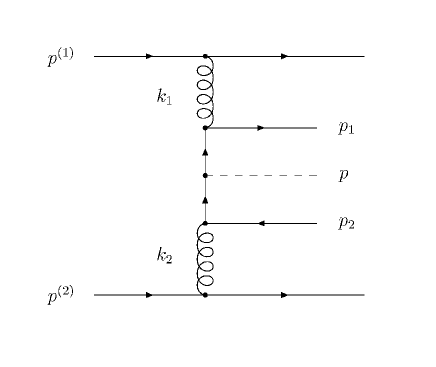
Figure 1: Kinematics of the $g^{*}+g^{*}\to W^{\pm}/Z^{0}+qq^{\prime}$ process.

We start from the kinematics (see Fig. 1). Let $p^{(1)}$ and $p^{(2)}$ be the four-momenta of the incoming protons and $p$ the four-momentum of the produced $W^{\pm}$/$Z^{0}$ boson. The initial off-shell gluons have the four-momenta $k_{1}$ and $k_{2}$ and the final quark $q$ and antiquark $\bar{q}^{\prime}$ have the four-momenta $p_{1}$ and $p_{2}$ and the masses $m_{1}$ and $m_{2}$, respectively. In the $p\bar{p}$ center-of-mass frame we can write

$$p^{(1)}={\sqrt{s}\over 2}(1,0,0,1),\quad p^{(2)}={\sqrt{s}\over 2}(1,0,0,-1),$$

where $\sqrt{s}$ is the total energy of the process under consideration and we neglect the masses of the incoming protons. The initial gluon four-momenta in the high energy limit can be written as

$$k_{1}=x_{1}p^{(1)}+k_{1T},\quad k_{2}=x_{2}p^{(2)}+k_{2T},$$

where $k_{1T}$ and $k_{2T}$ are the transverse four-momenta. It is important that ${\mathbf{k}}_{1T}^{2}=-k_{1T}^{2}\neq 0$ and ${\mathbf{k}}_{2T}^{2}=-k_{2T}^{2}\neq 0$. From the conservation laws we can obtain the following relations:

$${\mathbf{k}}_{1T}+{\mathbf{k}}_{2T}={\mathbf{p}}_{1T}+{\mathbf{p}}_{2T}+{\mathbf{p}}_{T},$$

$$x_{1}\sqrt{s}=m_{1T}e^{y_{1}}+m_{2T}e^{y_{2}}+m_{T}e^{y},$$

$$x_{2}\sqrt{s}=m_{1T}e^{-y_{1}}+m_{2T}e^{-y_{2}}+m_{T}e^{-y},$$

where $p_{T}$, $m_{T}$ and $y$ are the transverse momentum, transverse mass and center-of-mass rapidity of produced $W^{\pm}$/$Z^{0}$ boson, $p_{1T}$ and $p_{2T}$ are the transverse momenta of final quark $q$ and antiquark $\bar{q}^{\prime}$, $y_{1}$, $y_{2}$, $m_{1T}$ and $m_{2T}$ are their rapidities and transverse masses, i.e. $m_{iT}^{2}=m_{i}^{2}+{\mathbf{p}}_{iT}^{2}$.

2.2 Off-shell amplitude of the $g^{*}+g^{*}\to W^{\pm}/Z^{0}+q\bar{q}^{\prime}$ subprocess

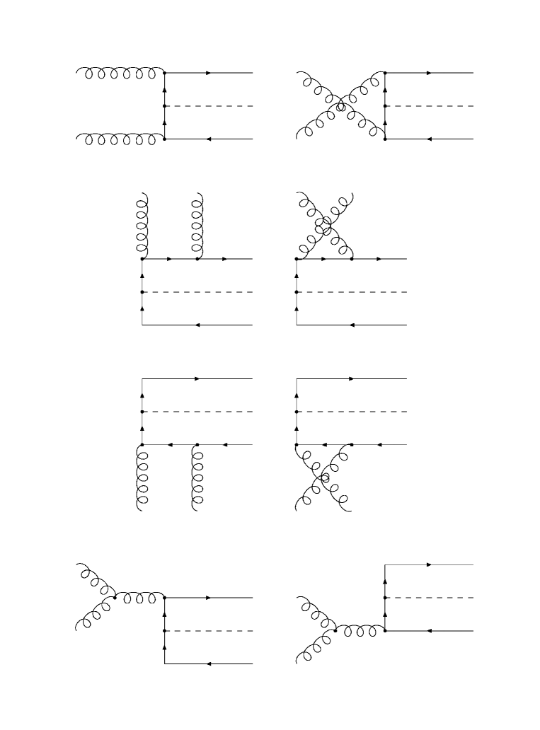
Figure 2: Feynman diagrams which describe the partonic subprocess $g^{*}+g^{*}\to W^{\pm}/Z^{0}+qq^{\prime}$ at the leading order in $\alpha_{s}$ and $\alpha$.

There are eight Feynman diagrams (see Fig. 2) which describe the partonic subprocess $g^{*}+g^{*}\to W^{\pm}/Z^{0}+q\bar{q}^{\prime}$ at $\alpha\alpha_{s}^{2}$ order. Let $\epsilon_{1}$, $\epsilon_{2}$ and $\epsilon$ be the initial gluon and produced gauge boson polarization vectors, respectively, and $a$ and $b$ the eight-fold color indices of the off-shell gluons. Then the relevant matrix element can be presented as follows:

$${\cal M}_{1}=g^{2}\,\bar{u}(p_{1})\,t^{a}\gamma^{\mu}\epsilon_{\mu}{\hat{p}_{1}-\hat{k}_{1}+m_{1}\over m_{1}^{2}-(p_{1}-k_{1})^{2}}T_{W,Z}^{\lambda}\,\epsilon_{\lambda}{\hat{k}_{2}-\hat{p}_{2}+m_{2}\over m_{2}^{2}-(k_{2}-p_{2})^{2}}t^{b}\gamma^{\nu}\epsilon_{\nu}\,u(p_{2}),$$

$${\cal M}_{2}=g^{2}\,\bar{u}(p_{1})\,t^{b}\gamma^{\nu}\epsilon_{\nu}{\hat{p}_{1}-\hat{k}_{2}+m_{1}\over m_{1}^{2}-(p_{1}-k_{2})^{2}}T_{W,Z}^{\lambda}\,\epsilon_{\lambda}{\hat{k}_{1}-\hat{p}_{2}+m_{2}\over m_{2}^{2}-(k_{1}-p_{2})^{2}}t^{a}\gamma^{\mu}\epsilon_{\mu}\,u(p_{2}),$$

$${\cal M}_{3}=g^{2}\,\bar{u}(p_{1})\,t^{a}\gamma^{\mu}\epsilon_{\mu}{\hat{p}_{1}-\hat{k}_{1}+m_{1}\over m_{1}^{2}-(p_{1}-k_{1})^{2}}\,t^{b}\gamma^{\nu}\epsilon_{\nu}{-\hat{p}_{2}-\hat{p}+m_{1}\over m_{1}^{2}-(-p_{2}-p)^{2}}T_{W,Z}^{\lambda}\,\epsilon_{\lambda}\,u(p_{2}),$$

$${\cal M}_{4}=g^{2}\,\bar{u}(p_{1})\,t^{b}\gamma^{\nu}\epsilon_{\nu}{\hat{p}_{1}-\hat{k}_{2}+m_{1}\over m_{1}^{2}-(p_{1}-k_{2})^{2}}\,t^{a}\gamma^{\mu}\epsilon_{\mu}{-\hat{p}_{2}-\hat{p}+m_{1}\over m_{1}^{2}-(-p_{2}-p)^{2}}T_{W,Z}^{\lambda}\,\epsilon_{\lambda}\,u(p_{2}),$$

$${\cal M}_{5}=g^{2}\,\bar{u}(p_{1})\,T_{W,Z}^{\lambda}\,\epsilon_{\lambda}{\hat{p}_{1}+\hat{p}+m_{2}\over m_{2}^{2}-(p_{1}+p)^{2}}\,t^{b}\gamma^{\nu}\epsilon_{\nu}{\hat{k}_{1}-\hat{p}_{2}+m_{2}\over m_{2}^{2}-(k_{1}-p_{2})^{2}}t^{a}\gamma^{\mu}\epsilon_{\mu}\,u(p_{2}),$$

$${\cal M}_{6}=g^{2}\,\bar{u}(p_{1})\,T_{W,Z}^{\lambda}\,\epsilon_{\lambda}{\hat{p}_{1}+\hat{p}+m_{2}\over m_{2}^{2}-(p_{1}+p)^{2}}\,t^{a}\gamma^{\mu}\epsilon_{\mu}{\hat{k}_{2}-\hat{p}_{2}+m_{2}\over m_{2}^{2}-(k_{2}-p_{2})^{2}}t^{b}\gamma^{\nu}\epsilon_{\nu}\,u(p_{2}),$$

$${\cal M}_{7}=g^{2}\,\bar{u}(p_{1})\,\gamma^{\rho}C^{\mu\nu\rho}(k_{1},k_{2},-k_{1}-k_{2}){\epsilon_{\mu}\epsilon_{\nu}\over(k_{1}+k_{2})^{2}}f^{abc}t^{c}\times\atop\displaystyle\times{-\hat{p}_{2}-\hat{p}+m_{1}\over m_{1}^{2}-(-p_{2}-p)^{2}}\,T_{W,Z}^{\lambda}\,\epsilon_{\lambda}\,u(p_{2}),$$

$${\cal M}_{8}=g^{2}\,\bar{u}(p_{1})\,T_{W,Z}^{\lambda}\,\epsilon_{\lambda}{\hat{p}_{1}+\hat{p}+m_{2}\over m_{2}^{2}-(p_{1}+p)^{2}}\times\atop\displaystyle\times\gamma^{\rho}C^{\mu\nu\rho}(k_{1},k_{2},-k_{1}-k_{2}){\epsilon_{\mu}\epsilon_{\nu}\over(k_{1}+k_{2})^{2}}f^{abc}t^{c}\,u(p_{2}).$$

In the above expressions $C^{\mu\nu\rho}(k,p,q)$ and $T_{W,Z}^{\lambda}$ are related to the standard QCD three-gluon coupling and the $W^{\pm}$/$Z^{0}$-fermion vertexes:

$$C^{\mu\nu\rho}(k,p,q)=g^{\mu\nu}(p-k)^{\rho}+g^{\nu\rho}(q-p)^{\mu}+g^{\rho\mu}(k-q)^{\nu},$$

$$T^{\lambda}_{W}={e\over 2\sqrt{2}\sin\theta_{W}}\gamma^{\lambda}(1-\gamma^{5})V_{qq^{\prime}},$$

$$T^{\lambda}_{Z}={e\over\sin 2\theta_{W}}\gamma^{\lambda}\left[I_{3}^{(q)}(1-\gamma^{5})-2e_{q}\sin^{2}\theta_{W}\right],$$

where $I_{3}^{(q)}$ and $e_{q}$ are the weak isospin and the fractional electric charge (in the positron charge $e$ units) of final-state quark $q$, $\theta_{W}$ is the Weinberg mixing angle and $V_{qq^{\prime}}$ is the Cabibbo-Kobayashi-Maskawa (CKM) matrix element. Of course, in the case of $Z^{0}$ production $m_{1}$ equals $m_{2}$. The summation on the $W^{\pm}$/$Z^{0}$ polarization is carried out by the covariant formula

$$\sum\epsilon^{\mu}(p)\,\epsilon^{*\,\nu}(p)=-g^{\mu\nu}+{p^{\mu}p^{\nu}\over m^{2}}.$$

In the case of the initial off-shell gluon we use the BFKL prescription [23, 24]:

$$\sum\epsilon^{\mu}(k_{i})\,\epsilon^{*\,\nu}(k_{i})={k_{iT}^{\mu}k_{iT}^{\nu}\over{\mathbf{k}}_{iT}^{2}}.$$

This formula converges to the usual expression $\sum\epsilon^{\mu}\epsilon^{*\,\nu}=-g^{\mu\nu}$ after azimuthal angle averaging in the $k_{T}\to 0$ limit. The evaluation of the traces in (4) — (11) was done using the algebraic manipulation system Form [34]. We would like to mention here that the usual method of squaring of (4) — (11) results in enormously long output. This technical problem was solved by applying the method of orthogonal amplitudes [35].

The gauge invariance of the matrix element is a subject of special attention in the $k_{T}$-factorization approach. Strictly speaking, the diagrams shown in Fig. 2 are insufficient and have to be accompanied with the graphs involving direct gluon exchange between the protons (these protons are not shown in Fig. 2). These graphs are necessary to maintain the gauge invariance. However, they violate the factorization since they cannot be represented as a convolution of the gluon-gluon fusion matrix element with unintegrated gluon density. The solution pointed out in [24] refers to the fact that, within the particular gauge (16), the contribution from these unfactorizable diagrams vanish, and one has to only take into account the graphs depicted in Fig. 2. We have successfully tested the gauge invariance of the matrix element (4) — (11) numerically.

2.3 Cross section for the inclusive $W^{\pm}$/$Z^{0}$ production

According to the $k_{T}$-factorization theorem, the inclusive $W^{\pm}$/$Z^{0}$ production cross section via two off-shell gluon fusion can be written as a convolution

$$\sigma(p+\bar{p}\to W^{\pm}/Z^{0}+X)=\sum_{q}\int{dx_{1}\over x_{1}}f_{g}(x_{1},{\mathbf{k}}_{1T}^{2},\mu^{2})d{\mathbf{k}}_{1T}^{2}{d\phi_{1}\over 2\pi}\times\atop\displaystyle\times\int{dx_{2}\over x_{2}}f_{g}(x_{2},{\mathbf{k}}_{2T}^{2},\mu^{2})d{\mathbf{k}}_{2T}^{2}{d\phi_{2}\over 2\pi}d{\hat{\sigma}}(g^{*}+g^{*}\to W^{\pm}/Z^{0}+q\bar{q}^{\prime}),$$

where $\hat{\sigma}(g^{*}+g^{*}\to W^{\pm}/Z^{0}+q\bar{q}^{\prime})$ is the partonic cross section, $f_{g}(x,{\mathbf{k}}_{T}^{2},\mu^{2})$ is the unintegrated gluon distribution in a proton and $\phi_{1}$ and $\phi_{2}$ are the azimuthal angles of the incoming gluons. The multiparticle phase space $\Pi d^{3}p_{i}/2E_{i}\delta^{(4)}(\sum p^{\rm in}-\sum p^{\rm out})$ is parametrized in terms of transverse momenta, rapidities and azimuthal angles:

$${d^{3}p_{i}\over 2E_{i}}={\pi\over 2}\,d{\mathbf{p}}_{iT}^{2}\,dy_{i}\,{d\phi_{i}\over 2\pi}.$$

Using the expressions (17) and (18) we obtain the master formula:

$$\sigma(p+\bar{p}\to W^{\pm}/Z^{0}+X)=\sum_{q}\int{1\over 256\pi^{3}(x_{1}x_{2}s)^{2}}|\bar{\cal M}(g^{*}+g^{*}\to W^{\pm}/Z^{0}+q\bar{q}^{\prime})|^{2}\times\atop\displaystyle\times f_{g}(x_{1},{\mathbf{k}}_{1T}^{2},\mu^{2})f_{g}(x_{2},{\mathbf{k}}_{2T}^{2},\mu^{2})d{\mathbf{k}}_{1T}^{2}d{\mathbf{k}}_{2T}^{2}d{\mathbf{p}}_{1T}^{2}{\mathbf{p}}_{2T}^{2}dydy_{1}dy_{2}{d\phi_{1}\over 2\pi}{d\phi_{2}\over 2\pi}{d\psi_{1}\over 2\pi}{d\psi_{2}\over 2\pi},$$

where $|\bar{\cal M}(g^{*}+g^{*}\to W^{\pm}/Z^{0}+q\bar{q}^{\prime})|^{2}$ is the off-mass shell matrix element squared and averaged over initial gluon polarizations and colors, $\psi_{1}$ and $\psi_{2}$ are the azimuthal angles of the final state quark and antiquark, respectively. We would like to point out again that $|\bar{\cal M}(g^{*}+g^{*}\to W^{\pm}/Z^{0}+q\bar{q}^{\prime})|^{2}$ strongly depends on the nonzero transverse momenta ${\mathbf{k}}_{1T}^{2}$ and ${\mathbf{k}}_{2T}^{2}$. If we average the expression (19) over $\phi_{1}$ and $\phi_{2}$ and take the limit ${\mathbf{k}}_{1T}^{2}\to 0$ and ${\mathbf{k}}_{2T}^{2}\to 0$, then we recover the expression for the $W^{\pm}$/$Z^{0}$ production cross section in the collinear $\alpha\alpha_{s}^{2}$ approximation.

The multidimensional integration in (19) has been performed by means of the Monte Carlo technique, using the routine Vegas [36]. The full C$++$ code is available from the authors upon request.

2.4 The KMR unintegrated parton distributions

In the present paper we have tried two different sets of unintegrated parton densities in a proton. First of them is the Kimber-Martin-Ryskin set.

The KMR approach [31] is the formalism to construct parton distributions $f_{a}(x,{\mathbf{k}}_{T}^{2},\mu^{2})$ unintegrated over the parton transverse momenta ${\mathbf{k}}_{T}^{2}$ from the known conventional parton distributions $xa(x,\mu^{2})$, where $a=g$ or $a=q$. This formalism is valid for a proton as well as a photon and can embody both DGLAP and BFKL contributions. It also accounts for the angular ordering which comes from coherence effects in gluon emission. The key observation here is that the $\mu$ dependence of the unintegrated parton distributions $f_{a}(x,{\mathbf{k}}_{T}^{2},\mu^{2})$ enters at the last step of the evolution, and therefore single scale evolution equations (pure DGLAP) can be used up to this step. In this approximation, the unintegrated quark and gluon distributions are given by the expressions [31]

$$f_{q}(x,{\mathbf{k}}_{T}^{2},\mu^{2})=T_{q}({\mathbf{k}}_{T}^{2},\mu^{2}){\alpha_{s}({\mathbf{k}}_{T}^{2})\over 2\pi}\times\atop{\displaystyle\times\int\limits_{x}^{1}dz\left[P_{qq}(z){x\over z}q\left({x\over z},{\mathbf{k}}_{T}^{2}\right)\Theta\left(\Delta-z\right)+P_{qg}(z){x\over z}g\left({x\over z},{\mathbf{k}}_{T}^{2}\right)\right],}$$

$$f_{g}(x,{\mathbf{k}}_{T}^{2},\mu^{2})=T_{g}({\mathbf{k}}_{T}^{2},\mu^{2}){\alpha_{s}({\mathbf{k}}_{T}^{2})\over 2\pi}\times\atop{\displaystyle\times\int\limits_{x}^{1}dz\left[\sum_{q}P_{gq}(z){x\over z}q\left({x\over z},{\mathbf{k}}_{T}^{2}\right)+P_{gg}(z){x\over z}g\left({x\over z},{\mathbf{k}}_{T}^{2}\right)\Theta\left(\Delta-z\right)\right],}$$

where $P_{ab}(z)$ are the usual unregulated leading order DGLAP splitting functions, and $q(x,\mu^{2})$ and $g(x,\mu^{2})$ are the conventional quark and gluon densities. The theta functions which appear in (20) and (21) imply the angular-ordering constraint $\Delta=\mu/(\mu+|{\mathbf{k}}_{T}|)$ specifically to the last evolution step to regulate the soft gluon singularities. For other evolution steps, the strong ordering in transverse momentum within the DGLAP equations automatically ensures angular ordering. It is important that the parton distributions $f_{a}(x,{\mathbf{k}}_{T}^{2},\mu^{2})$ extended now into the ${\mathbf{k}}_{T}^{2}>\mu^{2}$ region. This fact is in the clear contrast with the usual DGLAP evolution.

The virtual (loop) contributions may be resummed to all orders by the quark and gluon Sudakov form factors

$$\ln T_{q}({\mathbf{k}}_{T}^{2},\mu^{2})=-\int\limits_{{\mathbf{k}}_{T}^{2}}^{\mu^{2}}{d{\mathbf{p}}_{T}^{2}\over{\mathbf{p}}_{T}^{2}}{\alpha_{s}({\mathbf{p}}_{T}^{2})\over 2\pi}\int\limits_{0}^{z_{\rm max}}dzP_{qq}(z),$$

$$\ln T_{g}({\mathbf{k}}_{T}^{2},\mu^{2})=-\int\limits_{{\mathbf{k}}_{T}^{2}}^{\mu^{2}}{d{\mathbf{p}}_{T}^{2}\over{\mathbf{p}}_{T}^{2}}{\alpha_{s}({\mathbf{p}}_{T}^{2})\over 2\pi}\left[n_{f}\int\limits_{0}^{1}dzP_{qg}(z)+\int\limits_{z_{\rm min}}^{z_{\rm max}}dzzP_{gg}(z)\right],$$

where $z_{\rm max}=1-z_{\rm min}={\mu/({\mu+|{\mathbf{p}}_{T}|}})$. The form factors $T_{a}({\mathbf{k}}_{T}^{2},\mu^{2})$ give the probability of evolving from a scale ${\mathbf{k}}_{T}^{2}$ to a scale $\mu^{2}$ without parton emission. In according with (22) and (23) $T_{a}({\mathbf{k}}_{T}^{2},\mu^{2})=1$ in the ${\mathbf{k}}_{T}^{2}>\mu^{2}$ region.

Note that such definition of the $f_{a}(x,{\mathbf{k}}_{T}^{2},\mu^{2})$ is correct for ${\mathbf{k}}_{T}^{2}>\mu_{0}^{2}$ only, where $\mu_{0}\sim 1$ GeV is the minimum scale for which DGLAP evolution of the collinear parton densities is valid. Everywhere in our numerical calculations we set the starting scale $\mu_{0}$ to be equal $\mu_{0}=1$ GeV. Since the starting point of this derivation is the leading order DGLAP equations, the unintegrated parton distributions must satisfy the normalisation condition

$$a(x,\mu^{2})=\int\limits_{0}^{\mu^{2}}f_{a}(x,{\mathbf{k}}_{T}^{2},\mu^{2})d{\mathbf{k}}_{T}^{2}.$$

This relation will be exactly satisfied if one define [31]

$$f_{a}(x,{\mathbf{k}}_{T}^{2},\mu^{2})|_{{\mathbf{k}}_{T}^{2}<\mu_{0}^{2}}=a(x,\mu_{0}^{2})T_{a}(\mu_{0}^{2},\mu^{2}).$$

2.5 The CCFM unintegrated gluon distribution

The CCFM gluon density has been obtained [38] from the numerical solution of the CCFM equation. The function $f_{g}(x,{\mathbf{k}}_{T}^{2},\mu^{2})$ is determined by a convolution of the non-perturbative starting distribution $f_{g}^{(0)}(x)$ and the CCFM evolution kernel denoted by $\tilde{\cal A}(x,{\mathbf{k}}_{T}^{2},\mu^{2})$:

$$f_{g}(x,{\mathbf{k}}_{T}^{2},\mu^{2})=\int{dx^{\prime}\over x^{\prime}}f_{g}^{(0)}(x^{\prime})\tilde{\cal A}\left({x\over x^{\prime}},{\mathbf{k}}_{T}^{2},\mu^{2}\right).$$

In the perturbative evolution the gluon splitting function $P_{gg}(z)$ including nonsingular terms is applied, as it was described in [39]. The input parameters in $f_{g}^{(0)}(x)$ were fitted to reproduce the proton structure functions $F_{2}(x,Q^{2})$. An acceptable fit to the measured $F_{2}$ values was obtained [38] with $\chi^{2}/ndf=1.83$ using statistical and uncorrelated systematic uncertainties (compare to $\chi^{2}/ndf\sim 1.5$ in the collinear approach at NLO).

3 Numerical results

We are now in a position to present our numerical results. First we describe the theoretical uncertainties of our consideration.

Except the unintegrated parton distributions in a proton $f_{q}(x,{\mathbf{k}}_{T}^{2},\mu^{2})$, there are several parameters which determined the overall normalization factor of the calculated $W^{\pm}/Z^{0}$ cross sections: the quark masses $m_{1}$ and $m_{2}$ and the factorization and renormalization scales $\mu_{F}$ and $\mu_{R}$ (the first of them is related to the evolution of the parton distributions, the other is responsible for the strong coupling constant). In the numerical calculations the masses of light quarks were set to be equal to $m_{u}=4.5$ MeV, $m_{d}=8.5$ MeV, $m_{s}=155$ MeV and the charmed quark mass was set to $m_{c}=1.5$ GeV. We have checked that uncertainties which come from these quantities are negligible in comparison to the uncertainties connected with the scale and/or the unintegrated parton densities. As it is often done, we choose the renormalization and factorization scales to be equal: $\mu_{R}=\mu_{F}=\mu=\xi m_{T}$ (transverse mass of the produced vector boson). In order to investigate the scale dependence of our results we vary the scale parameter $\xi$ between $1/2$ and 2 about the default value $\xi=1$. For completeness, we set $m_{W}=80.403$ GeV, $m_{Z}=91.1876$ GeV, $\sin^{2}\theta_{W}=0.23122$ and use the LO formula for the strong coupling constant $\alpha_{s}(\mu^{2})$ with $n_{f}=4$ active quark flavors at $\Lambda_{\rm QCD}=200$ MeV (so that $\alpha_{s}(M_{Z}^{2})=0.1232$). Note that we use a special choice $\Lambda_{\rm QCD}=130$ MeV in the case of CCFM gluon ($\alpha_{s}(M_{Z}^{2})=0.1187$), as it was originally proposed in [38].

Before we proceed to the numerical results, we would like to comment on the effect of the higher order QCD contributions [30]. It is well-known that the leading-order $k_{T}$-factorization approach naturally includes a large part of them. It is a corrections which are kinematic in nature arising from the real parton emission during the evolution cascade. Another part of high-order contributions comes from the logarithmic loop corrections which have already been included in the Sudakov form factors (22) and (23). However, there are also the non-logarithmic loop corrections, arising, for example, from the gluon vertex corrections to Fig. 2. To take into account these contributions we will use the approach proposed in [30]. It was demonstrated that main part of the non-logarithmic loop corrections can be absorbed in the so-called K-factor given by the expression

$$K(q+\bar{q}^{\prime}\to W^{\pm}/Z^{0})\simeq\exp\left[C_{F}{\alpha_{s}(\mu^{2})\over 2\pi}\pi^{2}\right],$$

where color factor $C_{F}=4/3$. A particular choice $\mu^{2}={\mathbf{p}}_{T}^{4/3}m^{2/3}$ has been proposed [22, 30] to eliminate sub-leading logarithmic terms. We choose this scale to evaluate the strong coupling constant $\alpha_{s}(\mu^{2})$ in (27).

We begin the discussion by presenting a comparison between the different contributions to the $W^{\pm}/Z^{0}$ total cross section. The solid, dashed and dotted histograms in Figs. 3 — 6 represent the $g^{*}+g^{*}\to W^{\pm}/Z^{0}+q\bar{q}^{\prime}$, $q+q^{*}\to W^{\pm}/Z^{0}+q^{\prime}$ and $q+\bar{q}^{\prime}\to W^{\pm}/Z^{0}$ contributions to the rapidity distributions of gauge boson calculated at the Tevatron (Figs. 3 and 4) and LHC conditions (Figs. 5 and 6). It is important that in the last two subprocesses we take into account only the valence quarks within the usual collinear approximation. For illustration, we used here the KMR unintegrated gluon density. We found that the role of the gluon-gluon fusion subprocess is greatly increased at the LHC energy: it contributes only about 2 or 3% of the valence quark component at the Tevatron and more than 40% at the LHC. Moreover, in the last case it dominates over the valence contributions at the central rapidities. The contribution of the valence quark-antiquark annihilation subprocess is important at the Tevatron and gives only a few percents at the LHC energy. As expected, the contribution of the $q+g^{*}\to W^{\pm}/Z^{0}+q^{\prime}$ subprocess is significant in the forward rapidity region, $|y|>2$. At this point, we can conclude that the gluon-gluon fusion becomes an important production mechanism at high energies and therefore should be taken into account in the calculations. However, we would like to note that there is an additional contribution which is not included in the simple decomposition scheme proposed above. As it was mentioned above, in this scheme it was assumed that sea quarks appear only at last gluon splitting and there is no contribution from the quarks coming from the earlier steps of the evolution (and we absorb last step of the gluon ladder into hard matrix element $g^{*}+g^{*}\to W^{\pm}/Z^{0}+q\bar{q}^{\prime}$). It is not clear in advance, whether the last gluon splitting dominates or not. In order to model this additional component, we have repeated the calculations using the KMR unintegrated quark densities (20) and the quark-antiquark annihilation $q+\bar{q}^{\prime}\to W^{\pm}/Z^{0}$ matrix element. But in these evaluations we omited the last term and keep only sea quark in first term of (20). Thus, we switch off the pure gluon component of the sea quark distributions and remove the valence quarks from the evolution ladder. In this way only the contributions to the $f_{q}(x,{\mathbf{k}}_{T}^{2},\mu^{2})$ originating from the earlier (involving quarks) evolution steps are taken into account. So, the dash-dotted histograms in Figs. 3 — 6 represent the results of our calculations. We have found the significant (by about of 50%) enhancement of the cross sections at both the Tevatron and LHC conditions. Therefore in all calculations below we will consider this mechanism as an additional production one. Finally, taking into account all described above components, we can conclude that the gluon-gluon fusion contributes about $\sim 1$% to the total cross section at Tevatron and up to $\sim 25$% at LHC energies.

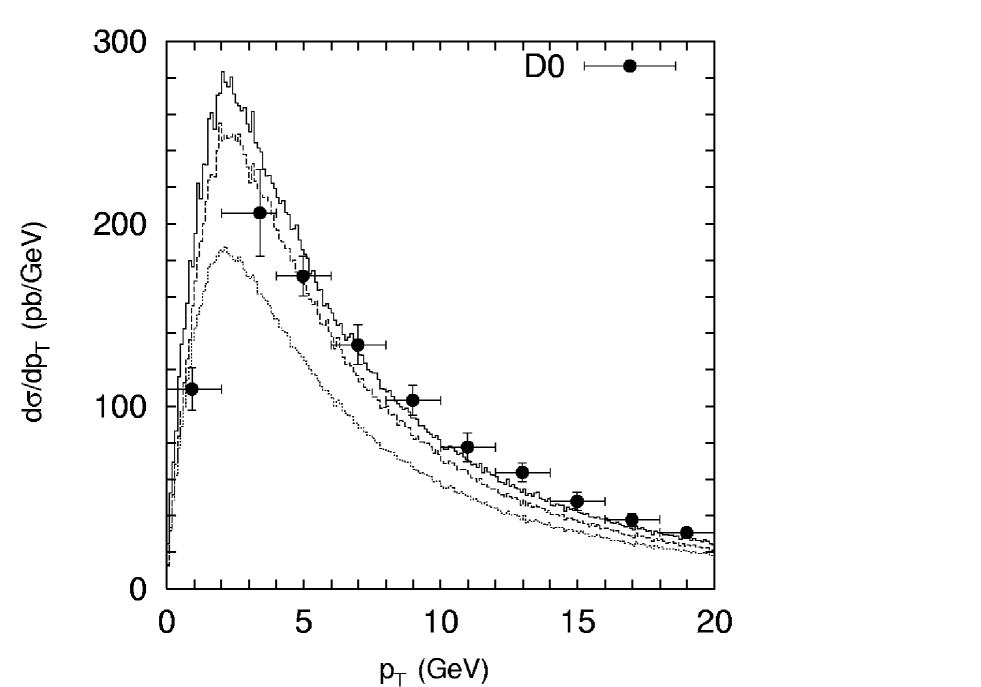
Figure 7: Transverse mometum distribution of the $W^{\pm}$ boson production. The solid and dashed histograms correspond to the results obtained with the CCFM and KMR unintegrated gluon densities in a proton, respectively. The dotted histograms were obtained by using the quark-antiquark annihilation matrix element convoluted with the KMR unintegrated quark distributions. The cross sections times branching fraction $f(W\to l\nu)$ are shown. The experimental data are from D$\oslash$ [9].

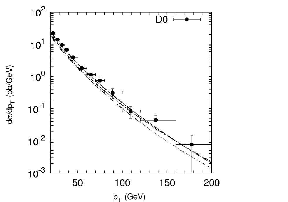
Figure 10: Transverse mometum distribution of the $W^{\pm}$ boson production. Notations of histograms are the same as in Fig. 7. The cross sections times branching fraction $f(W\to l\nu)$ are shown. The experimental data are from D$\oslash$ [9].

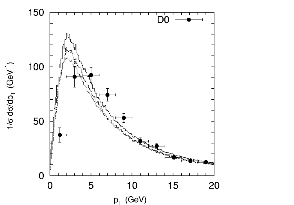
Figure 13: Normalized transverse mometum distribution of the $W^{\pm}$ boson production. Notations of histograms are the same as in Fig. 7. The earlier experimental data are from D$\oslash$ [5].

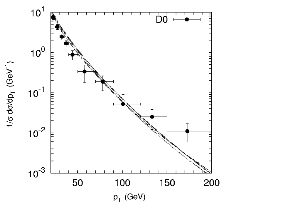
Figure 14: Normalized transverse mometum distribution of the $W^{\pm}$ boson production. Notations of histograms are the same as in Fig. 7. The earlier experimental data are from D$\oslash$ [5].

Now we turn to the transverse momentum distributions of the $W^{\pm}$ and $Z^{0}$ bosons. The experimental data for the transverse momentum distributions come from both the D$\oslash$ [8, 9] and CDF [4] collaborations at Tevatron. These data were obtained at center-of-mass energy $\sqrt{s}=1800$ GeV. Measurements were made for $W\to l\nu$ and $Z\to l^{+}l^{-}$ decays; so that we should multiply our theoretical predictions by the relevant branching fractions $f(W\to l\nu)$ and $f(Z\to l^{+}l^{-})$. These branching fractions were set to $f(W\to l\nu)=0.1075$ and $f(Z\to l^{+}l^{-})=0.03366$ [40]. In Figs. 7 — 9 we display a comparison of the calculated differential cross sections $d\sigma/dp_{T}$ of the $W^{\pm}$ and $Z^{0}$ boson production with the experimental data [4, 8, 9] in the low $p_{T}$ region, namely $p_{T}<20$ GeV. Next, in Figs. 10 — 12, we demonstrate the $W^{\pm}$ and $Z^{0}$ transverse momentum distributions in the intermediate and high $p_{T}$ regions. Additionally, in Figs. 13 and 14, we plot the normalized differential cross section $(1/\sigma)\,d\sigma/dp_{T}$ of the $W^{\pm}$ boson production. The solid and dashed histograms correspond to the results obtained with the CCFM and KMR unintegrated gluon densities, respectively. All contributions discussed above are taken into account. The dotted histograms were obtained using the quark-antiquark annihilation matrix element convoluted with the KMR unintegrated quark distributions in a proton (in this case the transverse mometum of the produced vector boson is defined by the transverse momenta of the incoming quarks). We found an increase in the cross section calculated in the proposed decomposition scheme (where only the unintegrated gluon densities used). In this scheme, we obtain that both the CCFM and KMR gluon distributions reproduce well the Tevatron data within the uncertainties, although the KMR gluon tends to slightly underestimate the data in the low $p_{T}$ region. The difference between the solid and dashed histograms in Figs. 7 — 14 is due to different behaviour of the CCFM and KMR gluon densities. The predictions based of the quark-antiquark annihilation subprocess lie below the experimental data but agree with them in shape. This observation coincides with the one from [30] where an additional factor of about 1.2 was introduced to eliminate the visible disagreement between the data and theory.

An additional possibility to distinguish the two calculation schemes comes from the studying of the ratio of the $W^{\pm}$ and $Z^{0}$ boson cross sections. In fact, since $W^{\pm}$ and $Z^{0}$ production properties are very similar, as the transverse momentum of the vector boson becomes smaller, the radiative corrections affecting the individual distributions and the cross sections of hard process are factorized and canceled in this ratio. Therefore the results of calculation of this ratio in the decomposition scheme (where the ${\cal O}(\alpha\alpha_{s})$ and ${\cal O}(\alpha\alpha_{s}^{2})$ subprocesses are taken into account) and the predictions based on the ${\cal O}(\alpha)$ quark-antiquark annihilation should differ from each other at moderate and high $p_{T}$ values. This fact is clearly illustrated in Fig. 15 where the ratio of $W^{\pm}$ and $Z^{0}$ cross sections as a function of the transverse momentum is displayed. As it was expected, there is practically no difference between all plotted histograms in the low $p_{T}$ region.

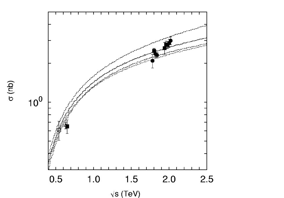
Figure 16: The total cross section of the inclusive $W^{\pm}$ boson production as a function of $\sqrt{s}$. The solid and dotted histograms correspond to the results obtained with the CCFM and KMR unintegrated gluon densities, respectively. The upper and lower dashed histograms correspond to the scale variations in CCFM gluon density as it was described in text. The cross sections times branching fraction $f(W\to l\nu)$ are shown. The experimental data are from UA1 [1], UA2[2], D$\oslash$ [6, 7] and CDF [3].

As a final point of our study, we discuss the scale dependence of our results. In Figs. 16 and 17 we show the total cross section of the $W^{\pm}$ and $Z^{0}$ boson production as a function of the total center-of-mass energy $\sqrt{s}$. Here, the solid and dotted histograms correspond to the results obtained with the CCFM and KMR unintegrated gluon densities, respectively. The the upper and lower dashed histograms correspond to the scale variations in the CCFM gluon density as it was described above. We find that the scale uncertainties are the same order approximately as the uncertainties coming from the unintegrated gluon distributions. This fact is the typical one for the leading-order $k_{T}$-factorization calculations. Our predictions for the $W^{\pm}$ and $Z^{0}$ boson total cross section agree well with the data in a wide $\sqrt{s}$ range.

4 Conclusions

We have studied the production of electroweak gauge bosons in hadronic collisions at high energies in the $k_{T}$-factorization approach of QCD. Our consideration is based on the scheme which provides solid theoretical grounds for adequately taking into account the effects of initial parton momentum. The central part of our derivation is the off-shell gluon-gluon fusion subprocess $g^{*}+g^{*}\to W^{\pm}/Z^{0}+q\bar{q}^{\prime}$. At the price of considering the corresponding matrix element rather than $q+\bar{q}^{\prime}\to W^{\pm}/Z^{0}$ one, we have reduced the problem of unknown unintegrated quark distributions to the problem of gluon distributions. This way enables us with making comparisons between the different parton evolution schemes and parametrizations of parton densities. Since the gluons are only responsible for the appearance of sea, but not valence quarks, the contribution from the valence quarks has been calculated separately. Having in mind that the valence quarks are only important at large $x$, where the traditional DGLAP evolution is accurate and reliable, we have calculated this contribution within the usual collinear scheme based on $q+g^{*}\to W^{\pm}/Z^{0}+q^{\prime}$ and $q+\bar{q}^{\prime}\to W^{\pm}/Z^{0}$ partonic subprocesses and on-shell parton densities.

We have studied in detail the different production mechanisms of $W^{\pm}$ and $Z^{0}$ bosons. We find that the off-shell gluon-gluon fusion gives $\sim 1$% and $\sim 25$% contributions to the inclusive $W^{\pm}/Z^{0}$ production cross sections at the Tevatron and LHC. Specially we simulate the contribution from the quarks involved into the earlier steps of the evolution cascade (i.e., into the second-to-last, third-to-last and other gluon splittings) and find that these quarks play an important role at both the Tevatron and LHC energies. It was demonstrated that corresponding corrections should be taken into accout in the numerical calculations within the $k_{T}$-factorization approach.

We have calculated the total and differential $W^{\pm}$ and $Z^{0}$ production cross sections and have made comparisons with the Tevatron data. In the numerical analysis we have used the unintegrated gluon densities obtained from the CCFM evolution equation and from the KMR prescription. Our numerical results agree well with the experimental data.

When the present paper was ready for publication, we have learned about the results obtained by M. Deak and F. Schwennsen [41], who used the same theoretical approach, but focused attention on slightly different aspects of the problem. These authors concentrate on the associated $W^{\pm}/Z^{0}$ production with heavy quark pairs (mainly on the $Zb\bar{b}$ final state), where the gluon-gluon fusion subprocess dominates. In additional to that, we consider quark subprocesses, which are important for inclusive $W^{\pm}/Z^{0}$ production. We show that the experimental data can be described with taking quark contributions into account.

5 Acknowledgements

We thank H. Jung for his encouraging interest, very helpful discussions and for providing the CCFM code for unintegrated gluon distributions. We thank M. Deak and F. Schwennsen for letting us know about the results of their work before publication and useful remarks. The authors are very grateful to DESY Directorate for the support in the framework of Moscow — DESY project on Monte-Carlo implementation for HERA — LHC. A.V.L. was supported in part by the grants of the president of Russian Federation (MK-438.2008.2) and Helmholtz — Russia Joint Research Group. Also this research was supported by the FASI of Russian Federation (grant NS-8122.2006.2) and the RFBR fundation (grant 08-02-00896-a).

6 Appendix A

Here we present the compact analytic expressions for the cross section of the $W^{\pm}/Z^{0}$ production via $q+\bar{q}^{\prime}\to W^{\pm}/Z^{0}$ subprocess in the $k_{T}$-factorization approach. Let us define the transverse momenta and azimuthal angles of incoming quark $q$ and antiquark $\bar{q}^{\prime}$ as ${\mathbf{k}}_{1T}$ and ${\mathbf{k}}_{2T}$ and $\phi_{1}$ and $\phi_{2}$, respectively. The produced vector boson has the transverse momentum ${\mathbf{p}}_{T}$ (${\mathbf{p}}_{T}={\mathbf{k}}_{1T}+{\mathbf{k}}_{2T}$) and center-of-mass rapidity $y$. The $W^{\pm}/Z^{0}$ production cross section can be written as

$$\sigma(p+\bar{p}\to W^{\pm}/Z^{0}+X)=\sum_{q}\int{2\pi\over(x_{1}x_{2}s)^{2}}|\bar{\cal M}(q+\bar{q}^{\prime}\to W^{\pm}/Z^{0})|^{2}\times\atop\displaystyle\times f_{q}(x_{1},{\mathbf{k}}_{1T}^{2},\mu^{2})f_{q}(x_{2},{\mathbf{k}}_{2T}^{2},\mu^{2})d{\mathbf{k}}_{1T}^{2}d{\mathbf{k}}_{2T}^{2}dy{d\phi_{1}\over 2\pi}{d\phi_{2}\over 2\pi},$$

where $f_{q}(x,{\mathbf{k}}_{T}^{2},\mu^{2})$ is the unintegrated quark distributions given by (20). In the high-energy limit the fractions $x_{1}$ and $x_{2}$ of the initial proton’s longitudinal momenta are given by

$$x_{1}\sqrt{s}=m_{T}\,e^{y},\quad x_{2}\sqrt{s}=m_{T}\,e^{-y}.$$

where $m_{T}$ is the transverse mass of the vector boson. The squared matrix element $|\bar{\cal M}(q+\bar{q}^{\prime}\to W^{\pm})|^{2}$ summed over final polarization states and averaged over initial ones is

$$|\bar{\cal M}(q+\bar{q}^{\prime}\to W^{\pm})|^{2}=-{e^{2}\over 72m_{W}^{2}\sin^{2}\theta_{W}}\left[(m_{1}^{2}-m_{2}^{2})^{2}+m_{W}^{2}(m_{1}^{2}+m_{2}^{2})-2m_{W}^{4}\right],$$

where $m_{1}$ and $m_{2}$ are the masses of incoming quarks. In the case of $Z^{0}$ boson production, the squared matrix element $|\bar{\cal M}(q+\bar{q}\to Z^{0})|^{2}$ summed over final polarization states and averaged over initial ones is

$$|\bar{\cal M}(q+\bar{q}\to Z^{0})|^{2}={2e^{2}\over 9\sin^{2}2\theta_{W}}\times\atop\displaystyle\times\left[(m_{Z}^{2}-m^{2})\left[I_{3}^{(q)}\right]^{2}+2e_{q}(2m^{2}+m_{Z}^{2})\sin^{2}\theta_{W}\left(e_{q}\sin^{2}\theta_{W}-I_{3}^{(q)}\right)\right],$$

where $m$, $e_{q}$ and $I_{3}^{(q)}$ is the mass, fractional electric charge and weak isospin of incoming quark. Note that there is no obvious dependence on the transverse momenta of the initial quark and antiquark. However, this dependence is present because the true off-shell kinematics is used. In particular, the incident parton momentum fractions $x_{1}$ and $x_{2}$ have some ${\mathbf{k}}_{T}$ dependence. If we take the limit ${\mathbf{k}}_{1T}^{2}\to 0$ and ${\mathbf{k}}_{2T}^{2}\to 0$, then we recover the relevant expression in the standard collinear approximation of QCD.

7 Appendix B

Here we present the analytic expressions for the cross section of the $W^{\pm}/Z^{0}$ production via $q+g^{*}\to W^{\pm}/Z^{0}+q^{\prime}$ subprocess in the $k_{T}$-factorization approach. Let us define the transverse momenta and azimuthal angles of incoming quark and off-shell gluon as ${\mathbf{k}}_{1T}$ and ${\mathbf{k}}_{2T}$ and $\phi_{1}$ and $\phi_{2}$, respectively. In the following, $\hat{s}$, $\hat{t}$ and $\hat{u}$ are usual Mandelstam variables for $2\to 2$ subprocess. The $W^{\pm}/Z^{0}$ production cross section can be written as follows:

$$\sigma(p+\bar{p}\to W^{\pm}/Z^{0}+X)=\sum_{q}\int{1\over 16\pi(x_{1}x_{2}s)^{2}}|\bar{\cal M}(q+g^{*}\to W^{\pm}/Z^{0}+q^{\prime})|^{2}\times\atop\displaystyle\times f_{q}(x_{1},{\mathbf{k}}_{1T}^{2},\mu^{2})f_{g}(x_{2},{\mathbf{k}}_{2T}^{2},\mu^{2})d{\mathbf{k}}_{1T}^{2}d{\mathbf{k}}_{2T}^{2}d{\mathbf{p}}_{T}^{2}dydy^{\prime}{d\phi_{1}\over 2\pi}{d\phi_{2}\over 2\pi},$$

where $y^{\prime}$ is the rapidity of the final quark $q^{\prime}$. The fractions $x_{1}$ and $x_{2}$ of the initial proton’s longitudinal momenta are given by

$$x_{1}\sqrt{s}=m_{T}\,e^{y}+m_{T}^{\prime}\,e^{y^{\prime}},\quad x_{2}\sqrt{s}=m_{T}\,e^{-y}+m_{T}^{\prime}\,e^{-y^{\prime}}.$$

where $m_{T}$ and $m_{T}^{\prime}$ are the transverse masses of the vector boson and final quark $q^{\prime}$. If we take the limit ${\mathbf{k}}_{1T}^{2}\to 0$ and ${\mathbf{k}}_{2T}^{2}\to 0$, then we recover the relevant expression in the usual collinear approximation. The squared matrix elements $|\bar{\cal M}(q+g^{*}\to W^{\pm}+q^{\prime})|^{2}$ and $|\bar{\cal M}(q+g^{*}\to Z^{0}+q)|^{2}$ summed over final polarization states and averaged over initial ones are

$$|\bar{\cal M}(q+g^{*}\to W^{\pm}+q^{\prime})|^{2}={e^{2}g^{2}\over 192\sin^{2}\theta_{W}}{F_{W}\over(m_{1}^{2}-\hat{s})^{2}(m_{2}^{2}-\hat{t})^{2}m_{W}^{2}},$$

$$|\bar{\cal M}(q+g^{*}\to Z^{0}+q)|^{2}={2e^{2}g^{2}\over 3\sin^{2}2\theta_{W}}{F_{Z}\over(m^{2}-\hat{s})^{2}(m^{2}-\hat{t})^{2}m_{Z}^{2}},$$

where

$$F_{W}=-8(m_{1}^{8}(3m_{2}^{2}-\hat{t})+m_{1}^{6}(m_{2}^{4}+m_{2}^{2}(2m_{W}^{2}-5\hat{s}-7\hat{t})+\hat{t}(\hat{s}+2\hat{t}))+$$

$$m_{1}^{4}(m_{2}^{6}+m_{2}^{4}(8m_{W}^{2}-3(\hat{s}+\hat{t}))+m_{2}^{2}(-6m_{W}^{4}+3\hat{s}^{2}+13\hat{s}\hat{t}+5\hat{t}^{2}-6m_{W}^{2}(\hat{s}+\hat{t}))-$$

$$\hat{t}(-2m_{W}^{4}-2m_{W}^{2}\hat{s}+(\hat{s}+\hat{t})^{2}))+m_{1}^{2}(3m_{2}^{8}+m_{2}^{6}(2m_{W}^{2}-7\hat{s}-5\hat{t})+$$

$$m_{2}^{4}(-6m_{W}^{4}+5\hat{s}^{2}+13\hat{s}\hat{t}+3\hat{t}^{2}-6m_{W}^{2}(\hat{s}+\hat{t}))+m_{2}^{2}(4m_{W}^{6}-\hat{s}^{3}-11\hat{s}^{2}\hat{t}-11\hat{s}\hat{t}^{2}-\hat{t}^{3}+$$

$$6m_{W}^{4}(\hat{s}+\hat{t})+6m_{W}^{2}(\hat{s}^{2}+\hat{t}^{2}))+\hat{t}(-4m_{W}^{6}+2m_{W}^{4}\hat{s}+\hat{s}(\hat{s}+\hat{t})^{2}-$$

$$2m_{W}^{2}(2\hat{s}^{2}-\hat{s}\hat{t}+\hat{t}^{2})))+\hat{s}(-m_{2}^{8}+m_{2}^{6}(2\hat{s}+\hat{t})+2m_{W}^{2}\hat{t}(2m_{W}^{4}+\hat{s}^{2}+\hat{t}^{2}-2m_{W}^{2}(\hat{s}+\hat{t}))+$$

$$m_{2}^{4}(2m_{W}^{4}+2m_{W}^{2}\hat{t}-(\hat{s}+\hat{t})^{2})+m_{2}^{2}(-4m_{W}^{6}+2m_{W}^{4}\hat{t}+\hat{t}(\hat{s}+\hat{t})^{2}-$$

$$2m_{W}^{2}(\hat{s}^{2}-\hat{s}\hat{t}+2\hat{t}^{2})))+(m_{1}^{8}+m_{2}^{8}+m_{1}^{6}(m_{W}^{2}-2(\hat{s}+\hat{t}))+m_{2}^{6}(m_{W}^{2}-2(\hat{s}+\hat{t}))+$$

$$m_{2}^{4}(-2m_{W}^{4}-2m_{W}^{2}\hat{t}+(\hat{s}+\hat{t})^{2})+m_{2}^{2}m_{W}^{2}(5\hat{s}^{2}+4\hat{s}\hat{t}+\hat{t}^{2}+m_{W}^{2}(-8\hat{s}+4\hat{t}))-$$

$$2m_{W}^{2}(2\hat{s}\hat{t}(\hat{s}+\hat{t})+m_{W}^{2}(\hat{s}^{2}-4\hat{s}\hat{t}+\hat{t}^{2}))+m_{1}^{4}(-2m_{2}^{4}-2m_{W}^{4}-2m_{W}^{2}\hat{s}+(\hat{s}+\hat{t})^{2}+$$

$$m_{2}^{2}(m_{W}^{2}+2(\hat{s}+\hat{t})))+m_{1}^{2}(m_{W}^{2}(\hat{s}^{2}+4m_{W}^{2}(\hat{s}-2\hat{t})+4\hat{s}\hat{t}+5\hat{t}^{2})+m_{2}^{4}(m_{W}^{2}+2(\hat{s}+\hat{t}))+$$

$$m_{2}^{2}(8m_{W}^{4}-6m_{W}^{2}(\hat{s}+\hat{t})-2(\hat{s}+\hat{t})^{2})))(-{\mathbf{k}}_{2T}^{2})+4m_{W}^{2}(m_{1}^{2}-\hat{s})(m_{2}^{2}-\hat{t}){\mathbf{k}}_{2T}^{4}),$$

$$F_{Z}=-2e_{q}I_{3}^{(q)}m_{Z}^{2}\sin^{2}\theta_{W}(6m^{8}-\hat{s}\hat{t}(2m_{Z}^{4}+\hat{s}^{2}+\hat{t}^{2}-2m_{Z}^{2}(\hat{s}+\hat{t}))-$$

$$m^{4}(2m_{Z}^{4}+3\hat{s}^{2}+14\hat{s}\hat{t}+3\hat{t}^{2}-2m_{Z}^{2}(\hat{s}+\hat{t}))+m^{2}(\hat{s}^{3}-8m_{Z}^{2}\hat{s}\hat{t}+7\hat{s}^{2}\hat{t}+$$

$$7\hat{s}\hat{t}^{2}+\hat{t}^{3}+2m_{Z}^{4}(\hat{s}+\hat{t})))+2e_{q}^{2}m_{Z}^{2}\sin^{4}\theta_{W}(6m^{8}-\hat{s}\hat{t}(2m_{Z}^{4}+\hat{s}^{2}+\hat{t}^{2}-2m_{Z}^{2}(\hat{s}+\hat{t}))-$$

$$m^{4}(2m_{Z}^{4}+3\hat{s}^{2}+14\hat{s}\hat{t}+3\hat{t}^{2}-2m_{Z}^{2}(\hat{s}+\hat{t}))+m^{2}(\hat{s}^{3}-8m_{Z}^{2}\hat{s}\hat{t}+7\hat{s}^{2}\hat{t}+7\hat{s}\hat{t}^{2}+\hat{t}^{3}+$$

$$2m_{Z}^{4}(\hat{s}+\hat{t})))+\left[I_{3}^{(q)}\right]^{2}(-4m^{10}+m^{8}(-6m_{Z}^{2}+8(\hat{s}+\hat{t}))-m_{Z}^{2}\hat{s}\hat{t}(2m_{Z}^{4}+\hat{s}^{2}+\hat{t}^{2}-$$

$$2m_{Z}^{2}(\hat{s}+\hat{t}))+m^{6}(6m_{Z}^{4}-5\hat{s}^{2}-14\hat{s}\hat{t}-5\hat{t}^{2}+6m_{Z}^{2}(\hat{s}+\hat{t}))+$$

$$m^{4}(-2m_{Z}^{6}+\hat{s}^{3}+7\hat{s}^{2}\hat{t}+7\hat{s}\hat{t}^{2}+\hat{t}^{3}-4m_{Z}^{4}(\hat{s}+\hat{t})-m_{Z}^{2}(3\hat{s}^{2}+2\hat{s}\hat{t}+3\hat{t}^{2}))+$$

$$m^{2}(-2m_{Z}^{4}\hat{s}\hat{t}+2m_{Z}^{6}(\hat{s}+\hat{t})-\hat{s}\hat{t}(\hat{s}+\hat{t})^{2}+m_{Z}^{2}(\hat{s}^{3}+\hat{s}^{2}\hat{t}+\hat{s}\hat{t}^{2}+\hat{t}^{3})))+$$

$$m_{Z}^{2}(2e_{q}I_{3}^{(q)}\sin^{2}\theta_{W}(2m^{4}(m_{Z}^{2}-\hat{s}-\hat{t})-2\hat{s}\hat{t}(\hat{s}+\hat{t})-m_{Z}^{2}(\hat{s}^{2}-4\hat{s}\hat{t}+\hat{t}^{2})-$$

$$2m^{2}(-4\hat{s}\hat{t}+m_{Z}^{2}(\hat{s}+\hat{t})))+2e_{q}^{2}\sin^{4}\theta_{W}(2\hat{s}\hat{t}(\hat{s}+\hat{t})+2m^{4}(-m_{Z}^{2}+\hat{s}+\hat{t})+$$

$$m_{Z}^{2}(\hat{s}^{2}-4\hat{s}\hat{t}+\hat{t}^{2})+2m^{2}(-4\hat{s}\hat{t}+m_{Z}^{2}(\hat{s}+\hat{t})))+\left[I_{3}^{(q)}\right]^{2}(-2m^{6}+2\hat{s}\hat{t}(\hat{s}+\hat{t})+$$

$$m_{Z}^{2}(\hat{s}^{2}-4\hat{s}\hat{t}+\hat{t}^{2})+m^{4}(-2m_{Z}^{2}+4(\hat{s}+\hat{t}))+m^{2}(-3\hat{s}^{2}-4\hat{s}\hat{t}-3\hat{t}^{2}+$$

$$2m_{Z}^{2}(\hat{s}+\hat{t}))))(-{\mathbf{k}}_{2T}^{2})-2m_{Z}^{2}(m^{2}-\hat{s})(\left[I_{3}^{(q)}\right]^{2}-$$

$$2e_{q}I_{3}^{(q)}\sin^{2}\theta_{W}+2e_{q}^{2}\sin^{4}\theta_{W})(m^{2}-\hat{t}){\mathbf{k}}_{2T}^{4}.$$

Figure 3: Different contributions to the inclusive $W^{\pm}$ boson production at the Tevatron conditions. The solid, dashed and dotted histograms correspond to the $g^{*}+g^{*}\to W^{\pm}+q\bar{q}^{\prime}$, $q+g^{*}\to W^{\pm}+q^{\prime}$ and $q+\bar{q}^{\prime}\to W^{\pm}$ subprocesses. In the last two cases only the valence quarks are taken into account. The dash-dotted histogram represents contribution from the quarks coming from the earlier steps of the evolution. The thick solid histogram represents the sum of all contributions. The KMR unintegrated parton densities in a proton are used.

Figure 4: Different contributions to the inclusive $Z^{0}$ boson production at the Tevatron conditions. Notations of histograms are the same as in Fig. 3.

Figure 5: Different contributions to the inclusive $W^{\pm}$ boson production at the LHC conditions. Notations of histograms are the same as in Fig. 3.

Figure 6: Different contributions to the inclusive $Z^{0}$ boson production at the LHC conditions. Notations of histograms are the same as in Fig. 3.

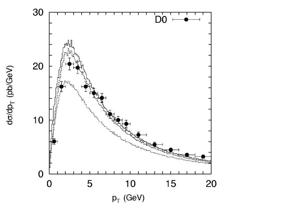
Figure 8: Transverse mometum distribution of the $Z^{0}$ boson production. Notations of histograms are the same as in Fig. 7. The cross sections times branching fraction $f(Z\to l^{+}l^{-})$ are shown. The experimental data are from D$\oslash$ [8].

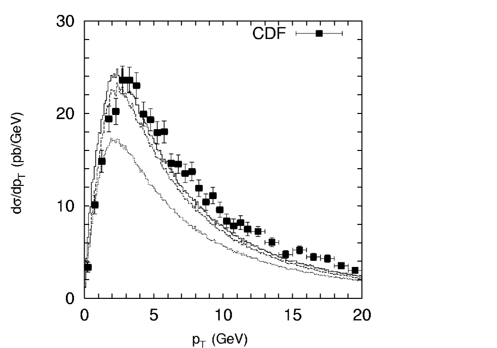
Figure 9: Transverse mometum distribution of the $Z^{0}$ boson production. Notations of histograms are the same as in Fig. 7. The cross sections times branching fraction $f(Z\to l^{+}l^{-})$ are shown. The experimental data are from CDF [4].

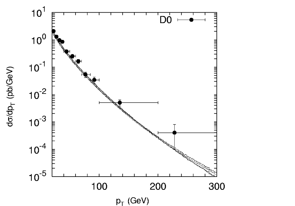
Figure 11: Transverse mometum distribution of the $Z^{0}$ boson production. Notations of histograms are the same as in Fig. 7. The cross sections times branching fraction $f(Z\to l^{+}l^{-})$ are shown. The experimental data are from D$\oslash$ [8].

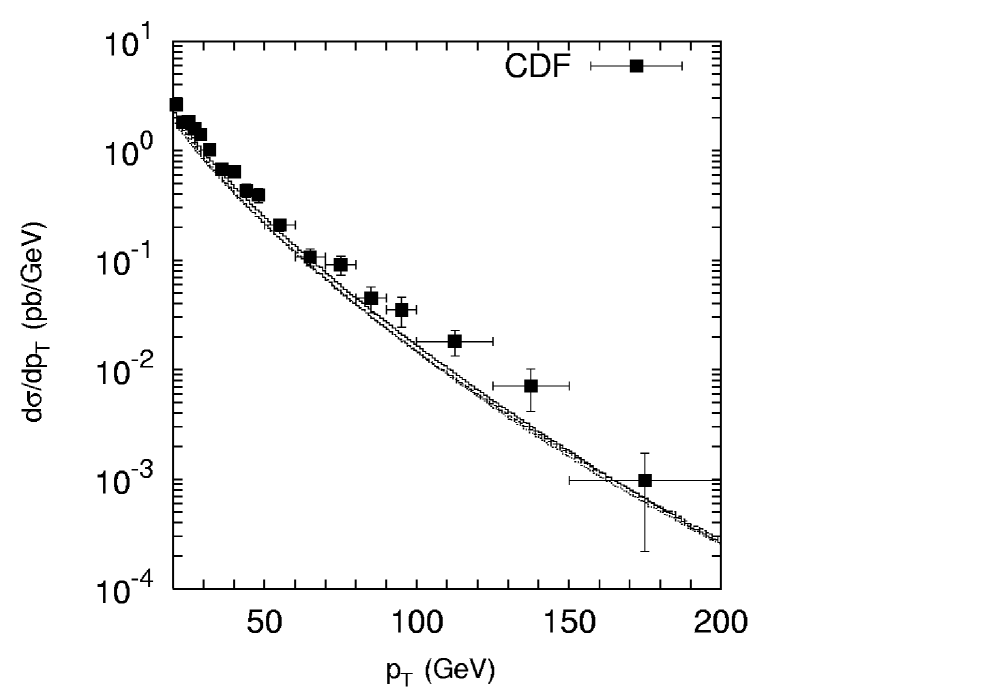
Figure 12: Transverse mometum distribution of the $Z^{0}$ boson production. Notations of histograms are the same as in Fig. 7. The cross sections times branching fraction $f(Z\to l^{+}l^{-})$ are shown. The experimental data are from CDF [4].

Figure 15: Ratio of differential cross section for $W^{\pm}$ to $Z^{0}$ production. Notations of histograms are the same as in Fig. 7. The experimental data are from D$\oslash$ [8].

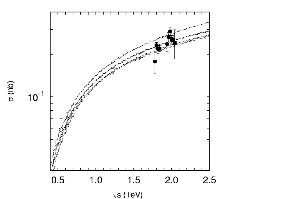
Figure 17: The total cross section of the inclusive $Z^{0}$ boson production as a function of $\sqrt{s}$. Notations of histograms are the same as in Fig. 16. The cross sections times branching fraction $f(Z\to l^{+}l^{-})$ are shown. The experimental data are from UA1 [1], UA2[2], D$\oslash$ [6, 7] and CDF [3].

References

- [1] C. Albajar et al. (UA1 Collaboration), Phys. Lett. B 253, 503 (1991).
- [2] J. Alitti et al. (UA2 Collaboration), Z. Phys. 47, 11 (1990).
- [3] F. Abe et al. (CDF Collaboration), Phys. Rev. Lett. 76, 3070 (1996).
- [4] B. Affolder et al. (CDF Collaboration), Phys. Rev. Lett. 84, 845 (2000).
- [5] B. Abbott et al. (D Collaboration), Phys. Rev. Lett. 80, 5498 (1998).
- [6] S. Abachi et al. (D Collaboration), Phys. Rev. Lett. 75, 1456 (1995).
- [7] B. Abbott et al. (D Collaboration), Phys. Rev. D 61, 072001 (2000).
- [8] B. Abbott et al. (D Collaboration), Phys. Rev. D 61, 032004 (2000).
- [9] B. Abbott et al. (D Collaboration), Phys. Lett. B 513, 292 (2001).
- [10] P. Sutton, A. Martin, R. Roberts, and W.J. Stirling, Phys. Rev. D 45, 2349 (1992).
- [11] R. Rijken and W. van Neerven, Phys. Rev. D 51, 44 (1995).
- [12] R. Hamberg, W. van Neerven, and T. Matsuura, Nucl. Phys. B 359, 343 (1991).
- [13] R. Harlander and W. Kilgore, Phys. Rev. Lett. 88, 201801 (2002).
- [14] W. van Neerven and E. Zijstra, Nucl. Phys. B 382, 11 (1992).
-
[15]
J. Collins, D. Soper, and G. Sterman, Nucl. Phys. B 250, 199 (1985);
J. Collins and D. Soper, Nucl. Phys. B 193, 381 (1981); Nucl. Phys. B 197, 446 (1982). -
[16]
C. Davies, B. Webber, and W.J. Stirling, Nucl. Phys. B 256, 413 (1985);
C. Davies and W.J. Stirling, Nucl. Phys. B 244, 337 (1984). - [17] G. Altarelli, R.K. Ellis, M. Grego, and G. Martinelli, Nucl. Phys. B 246, 12 (1984).
- [18] P.B. Arnold and R. Kauffman, Nucl. Phys. B 349, 381 (1991).
- [19] G.A. Ladinsky and C.P. Yuan, Phys. Rev. D 50, 4239 (1994).
- [20] R.K. Ellis and S. Veseli, Nucl. Phys. B 511, 649 (1998).
- [21] C. Balazs and C.P. Yuan, Phys. Rev. D 56, 5558 (1997).
- [22] A. Kulesza and W.J. Stirling, Nucl. Phys. B 555, 279 (1999).
-
[23]
L.V. Gribov, E.M. Levin, and M.G. Ryskin, Phys. Rep. 100, 1 (1983);
E.M. Levin, M.G. Ryskin, Yu.M. Shabelsky and A.G. Shuvaev, Sov. J. Nucl. Phys. 53, 657 (1991). -
[24]
S. Catani, M. Ciafoloni and F. Hautmann, Nucl. Phys. B 366, 135 (1991);
J.C. Collins and R.K. Ellis, Nucl. Phys. B 360, 3 (1991). -
[25]
E.A. Kuraev, L.N. Lipatov, and V.S. Fadin, Sov. Phys. JETP 44, 443 (1976);
E.A. Kuraev, L.N. Lipatov, and V.S. Fadin, Sov. Phys. JETP 45, 199 (1977);
I.I. Balitsky and L.N. Lipatov, Sov. J. Nucl. Phys. 28, 822 (1978). -
[26]
M. Ciafaloni, Nucl. Phys. B 296, 49 (1988);
S. Catani, F. Fiorani, and G. Marchesini, Phys. Lett. B 234, 339 (1990);
S. Catani, F. Fiorani, and G. Marchesini, Nucl. Phys. B 336, 18 (1990);
G. Marchesini, Nucl. Phys. B 445, 49 (1995). -
[27]
V.N. Gribov and L.N. Lipatov, Yad. Fiz. 15, 781 (1972);
L.N. Lipatov, Sov. J. Nucl. Phys. 20, 94 (1975);
G. Altarelli and G. Parisi, Nucl. Phys. B 126, 298 (1977);
Y.L. Dokshitzer, Sov. Phys. JETP 46, 641 (1977). - [28] A. Gawron and J. Kwiecinski, Phys. Rev. D 70, 014003 (2004).
-
[29]
B. Andersson et al. (Small- Collaboration), Eur. Phys. J. C 25, 77 (2002);
J. Andersen et al. (Small- Collaboration), Eur. Phys. J. C 35, 77 (2004);
J. Andersen et al. (Small- Collaboration), Eur. Phys. J. C 48, 53 (2006). - [30] G. Watt, A.D. Martin, and M.G. Ryskin, Phys. Rev. D 70, 014012 (2004).
-
[31]
M.A. Kimber, A.D. Martin, and M.G. Ryskin, Phys. Rev. D 63, 114027 (2001);
G. Watt, A.D. Martin, and M.G. Ryskin, Eur. Phys. J. C 31, 73 (2003). - [32] A.V. Bogdan and A.V. Grabovsky, Nucl. Phys. B 773, 65 (2007).
- [33] S.P. Baranov, A.V. Lipatov and N.P Zotov, Phys. Rev. D 77, 074024 (2008).
- [34] J.A.M. Vermaseren, ”Symbolic Manipulation with FORM”, published by Computer Algebra Nederland, Kruislaan 413, 1098, SJ Amsterdaam, 1991; ISBN 90-74116-01-9.
-
[35]
R.E. Prange, Phys. Rev. 110, 240 (1958);
S.P. Baranov, Phys. Atom. Nucl. 60, 1322 (1997). - [36] G.P. Lepage, J. Comput. Phys. 27, 192 (1978).
-
[37]
M. Glück, E. Reya and A. Vogt, Phys. Rev. D 46, 1973 (1992);
M. Glück, E. Reya and A. Vogt, Z. Phys. C 67, 433 (1995). - [38] H. Jung, A.V. Kotikov, A.V. Lipatov and N.P. Zotov, in Proceedings of ICHEP’06, p. 493 [hep-ph/0611093].
- [39] H. Jung, Mod. Phys. Lett. A 19, 1 (2004).
- [40] W.-M. Yao et al. (Particle Data Group), J. Phys. G 33, 1 (2006).
- [41] M. Deak and F. Schwennsen, arXiv:0805.3763 [hep-ph].