Local Density of States for Individual Energy Levels in Finite Quantum Wires

Abstract

The local density of states (LDOS) in finite quantum wires is calculated as a function of discrete energies and position along the wire. By using a combination of numerical density matrix renormalization group (DMRG) calculations and analytical bosonization techniques it is possible to obtain a good understanding of the local spectral weights along the wire in terms of the underlying many-body excitations.

There has been increasing interest in quasi one-dimensional quantum wires over the last few decades. Tunneling experiments have revealed signatures of strong correlations in different setups ranging from a powerlaw behavior of the temperature dependent conductance in carbon nanotubes Bockrath1999 ; Dekker1999 to being able to map out the momentum resolved tunneling in parallel quantum wires in a GaAs/AlGaAs heterostructure Auslaender2005 ; Auslaender2002 ; Steinberg2006 . By now the local tunneling density near nanotube edges can be measured fully resolved in energy and position Lee2004 , which has been interpreted as the interference pattern of collective excitations. Standing waves at discrete energies corresponding to the few lowest lying levels have also been observed in finite tubes with screened interactions venema ; lemay . It can be expected that similar experiments will be able to identify collective excitations in short finite wires if the screening from the substrate can be reduced.

The central quantity of interest is the local density of states (LDOS) of inserting one particle at position $x$ to reach an excited state $\langle\omega_{n}|$ with $N_{0}+1$ particles from the ground state $|N_{0}\rangle$

$$\rho(\omega,x) = \sum_{n}|\langle\omega_{n}|\psi^{\dagger}_{x}|N_{0}\rangle|^{2}\,\delta(\omega-\omega_{n})$$ (1)

$$= -\frac{1}{\pi}{\rm Im}\int_{0}^{\infty}e^{i\omega t}G^{R}(t,x)dt.$$

Using the Luttinger liquid formalism it is now well understood how the scaling laws of the LDOS and the correlation functions are affected by boundaries Eggert1992 ; Fabrizio1995 ; Eggert1996 ; Mattsson1997 ; Meden2000 ; Eggert2000 ; paata . The position resolved LDOS in finite wires was considered in Ref. [Anfuso2003, ] for the lowest few levels assuming a perfect degeneracy in the Luttinger liquid model.

From the numerical side it is surprising that so far only very few works Jeckelmann2004 were able to analyze the DOS in interacting lattice models exactly. Part of the difficulty appears to be that the LDOS in Eq. (1) is related to the time-dependent retarded Green’s function $G^{R}(t)$. In dynamical DMRG methods dramatic progress has been made over the past few years. Recently, it was possible to determine the spectral function as a function of the photoemission wavevector Jeckelmann2004 . Unfortunately, individual levels have not yet been resolved due to a finite correlation time or a finite cutoff in the Lehmann representation of the Green’s function. To our knowledge there have been no numerical calculations for the LDOS in interacting lattice models so far.

In this paper, we are now able to quantitatively calculate the LDOS of a finite quantum wire by using a combination of bosonization and DMRG techniques White1992 . In the numerical DMRG calculations we follow a direct approach, by targeting several excited states $\langle\omega_{n}|$ in the sector with one additional fermion on top of the ground state. Keeping track of the particle number and all the anticommuting transition operators $\psi^{\dagger}_{x}$ it is then possible to evaluate the matrix elements of the LDOS in Eq. (1) with very good spatial and energy resolution compared to calculating the DOS via the Green’s function. Using bosonization a general analytic formula for the LDOS of nearly degenerate states is derived. The combination of numerical and analytical calculations gives a good understanding of the distribution of spectral weights over individual states. The well-known powerlaws, however, can only be observed after a summation over nearly degenerate states. The effect of spin is also discussed.

We consider interacting spinless fermions hopping on a finite wire with $L$ sites and ”open” ($\psi_{0}=\psi_{L+1}=0$) boundary conditions

$$H=-t\sum_{x=1}^{L-1}\left(\psi^{\dagger}_{x}\psi^{\phantom{\dagger}}_{x+1}+h.c.\right)+U\sum_{x=1}^{L-1}n_{x}n_{x+1},$$ (2)

where $n_{x}=:\!\!\psi^{\dagger}_{x}\psi^{\phantom{\dagger}}_{x}\!\!:$. This is the simplest model that illustrates Luttinger liquid physics for $-2t<U\leq 2t$ and is often used to describe quantum wires. It is believed that the results can be generalized to systems with spin as will be discussed later. Tunneling one single particle (or hole) into the wire will create excited states that may in general involve several more fermions (i.e. a so-called ”single particle” excitation may still be a many-body entangled state). In order to illustrate the nature of such many-body excitations, consider the system without interaction $(U=0)$ first. In that case, eigenstates are created from the vacuum by creation operators $c_{n}^{\dagger}=\sqrt{\frac{2}{L+1}}\sum_{x}\psi_{x}^{\dagger}\sin(k_{n}+k_{F})x$, where the wavevector $k_{n}=n\frac{\pi}{L+1}$ is measured relative to the Fermi point $k_{F}$. For convenience $k_{F}=(N_{0}+1)\frac{\pi}{L+1}$ is chosen so that the number of particles in the filled Fermi sea is given by $N_{0}$ with energy $E_{0}$ and there is no charging energy to the $N_{0}+1$ particle sector as indicated in Fig. 1. A typical example of a single-particle excitation in a tunneling experiment is the creation of one fermion above the filled Fermi sea $|a\rangle=c_{2}^{\dagger}|N_{0}\rangle$ as shown in Fig. 1. In that case, the LDOS in Eq. (1) is simply given by the square of the corresponding standing wave. A second example of a possible excitation $|b\rangle=c_{1}^{\dagger}c_{0}^{\dagger}c_{-1}|N_{0}\rangle$ is shown in Fig. 1, where also one additional fermion is created and another one has been excited from the Fermi sea. For non-interacting fermions the overlap matrix elements $\langle b|\psi^{\dagger}_{x}|N_{0}\rangle$ of this many-body excited state vanish in the LDOS Eq. (1), but this is no longer true for the interacting case. Using numerical results and bosonization we are now able to describe quantitatively how spectral weight is shifted from ”simple excitations” (type $|a\rangle$) to many-body excited states (type $|b\rangle$) due to interactions and how this is reflected in the standing waves of the LDOS.

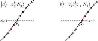
Figure 1: (color online) Single particle excitations on the filled Fermi sea for the non-interacting system.

Note, that if the dispersion relation was exactly linear, the states $|a\rangle$ and $|b\rangle$ would be degenerate. In fact a linear spectrum is often assumed, because in that case all many-body excitations are exactly quantized with energy levels $\omega_{n}=v_{F}k_{n}=\frac{v_{F}\pi}{L+1}n$ relative to $E_{0}$, where the number of possible partitions of $n=\sum_{\ell=1}^{\infty}\ell m_{\ell}$ into integers $m_{\ell}$ gives the degeneracy of the level $\omega_{n}$ (e.g. for $n=3=2+1=1+1+1$ there are three possible partitions). However, numerically we keep track of the exact spectrum of the finite lattice model, which is never exactly linear so that the degeneracies are lifted.

Even without assuming a linear spectrum the problem can be bosonized by defining shifting operators $\varrho_{n}=\sum_{\ell}c_{\ell+n}^{\dagger}c_{\ell}^{\phantom{\dagger}}$ for $n\neq 0$, which obey bosonic commutation relations $\left[\varrho_{-n},\varrho_{n^{\prime}}\right]=n\delta_{n,n^{\prime}}$ on the infinitely continued spectrum egg07 . The zero mode $\varrho_{0}=\sum_{\ell}\left(c_{\ell}^{\dagger}c_{\ell}^{\phantom{\dagger}}-\langle c_{\ell}^{\dagger}c_{\ell}^{\phantom{\dagger}}\rangle_{k_{F}}\right)$ counts the number of particles relative to the filled Fermi sea. It is possible to create any fermion state with a given particle number in terms of the $\varrho_{n}$. For example, we find by combinatorial methods that the addition of one fermion is represented by the following superposition of many-body bosonic states

$$c_{n}^{\dagger}|N_{0}\rangle=\sum_{\sum_{\ell}\ell m_{\ell}=n}\prod_{\ell}\frac{1}{m_{\ell}!}\left(\frac{\varrho_{\ell}}{\ell}\right)^{m_{\ell}}|0\rangle,$$ (3)

where $|0\rangle$ represents the ground state with $N_{0}+1$ fermions. Here, the sum runs over occupation numbers $m_{\ell}=\langle\varrho_{\ell}\varrho_{-\ell}\rangle/\ell$ which correspond to all possible partitions of $n=\sum_{\ell}\ell m_{\ell}$ schoenhammer . In particular, the states in Fig. 1 are given by

$$|a/b\rangle = \tfrac{1}{2}\left(\varrho_{1}^{2}\pm\varrho_{2}\right)|0\rangle.$$ (4)

The local addition of one fermion is described by $\psi^{\dagger}_{x}\approx e^{-ik_{F}x}\psi^{\dagger}_{R}(x)-e^{ik_{F}x}\psi^{\dagger}_{R}(-x)$, where

$$\psi_{R}^{\dagger}(x)=c(x)\exp{(\sum_{n>0}{e^{-ik_{n}x}}\frac{\varrho_{n}}{n})}\exp{(\sum_{n<0}{e^{-ik_{n}x}}\frac{\varrho_{n}}{n})}$$ (5)

in accordance with open boundary conditions Eggert1992 ; Fabrizio1995 ; Eggert1996 ; Mattsson1997 . Here, the prefactor $c(x)=\frac{i}{\sqrt{2(L+1)}}e^{i({\phi}_{0}-\varrho_{0}\frac{\pi x}{L+1})}$ also contains the zero mode operators $\varrho_{0}$ and $\phi_{0}$, which exactly create the $(N_{0}+1)$-particle ground state $|0\rangle=e^{i({\phi}_{0}-\varrho_{0}\frac{\pi x}{L+1})}|N_{0}\rangle$. The ambitious reader may enjoy verifying that the state in Eq. (3) is normalized and that the free fermion result $|\langle N_{0}|c_{n}\psi^{\dagger}_{x}|N_{0}\rangle|^{2}=\frac{2}{L+1}|\sin(k_{F}+k_{n})x|^{2}$ can also be evaluated in the boson language using Eq. (3) and (5).

Interactions $U$ can now be treated by a Bogoliubov transformation ${\varrho}_{n}=\alpha{\tilde{\varrho}}_{n}+\beta{\tilde{\varrho}}_{-n}$ where the rescaling parameters $\alpha=\frac{1}{2}(1/\sqrt{K}+\sqrt{K})$ and $\beta=\frac{1}{2}(1/\sqrt{K}-\sqrt{K})$ are characterized by the Luttinger liquid parameter $K$. For the model in Eq. (2), $K$ and the Fermi velocity $v_{F}$ are known exactly as a function of $U$ by comparison with Bethe ansatz, e.g. at half filling $1/2K=1-\arccos(U/2t)/\pi$ and $v_{F}=2tK\sin(\pi/2K)/(2K-1)$. The interacting Hamiltonian becomes diagonal $H=\frac{\pi{v}_{F}}{L+1}\sum_{\ell=1}^{\infty}\ell{\tilde{\varrho}}_{\ell}{\tilde{\varrho}}_{-\ell}$ up to non-linear corrections, which are described by higher order operators. After normal ordering the prefactor of the transformed fermion operator in Eq. (5) is given by

$$c(x)=\tfrac{i}{\sqrt{2(L+1)}}\left(\tfrac{\pi}{L+1}a\right)^{\beta^{2}}\left(2\sin\tfrac{\pi}{L+1}x\right)^{\alpha\beta},$$ (6)

where the inconsequential zero modes are left out. Here $a$ is a so-called cutoff parameter of order one lattice constant, which comes from a sum over physical states and can be determined numerically.

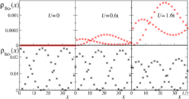
Figure 2: (Color online) DMRG data for the LDOS $|\langle b|\psi^{\dagger}(x)|N_{0}\rangle|^{2}$ (first row) and $|\langle a|\psi^{\dagger}(x)|N_{0}\rangle|^{2}$ for $L=78$, where $|b\rangle$ and $|a\rangle$ are eigenstates that have evolved from the $n=2$ states in Fig. 1 when interactions $U$ are switched on. The spectral weight is shifted towards $|b\rangle$ with increasing interactions, but $|a\rangle$ remains dominant.

The transformed boson vacuum and all eigenstates correspond to complicated many-fermion superpositions, which we can now analyze numerically. We implement the model in Eq. (2) with $L=78$ sites and $N_{0}+1=40$ using a multitarget DMRG. By keeping reflection and particle number symmetries, the position resolved matrix elements $\langle E|\psi^{\dagger}_{x}|N_{0}\rangle$ of 67 excited states $\langle E|$ are calculated. The eigenenergies $E$ agree to at least 8 digits with the exact Bethe ansatz.

We use the simplest example of the states $|a\rangle$ and $|b\rangle$ in order to illustrate how the LDOS changes with $U$ as shown in Fig. 2. The spectral weight of the many-body state $|b\rangle$ increases with interactions. The wavefunction can be analyzed with the help of Eq. (5), so that the eigenstates are known in terms of bosonic excitations, e.g. $|b\rangle\approx(0.541\tilde{\varrho}_{1}^{2}-0.455\tilde{\varrho}_{2})|0\rangle$ for $U=1.6t$.

The exact bosonic states are determined by higher order operators in the bosonized Hamiltonian, which are not known quantitatively. However, since the complete nearly degenerate subspace for a given energy $\omega_{n}=v_{F}k_{n}$ is known, it is in principle possible to calculate the sum of the LDOS of nearly degenerate states, i.e. $\rho_{n}(x)=\int_{\omega\approx\omega_{n}}\rho(\omega,x)d\omega$. By summing over bosonic eigenstates $\prod_{\ell=1}^{n}\left(\ell^{m_{\ell}}m_{\ell}!\right)^{-1/2}\tilde{\varrho}_{\ell}^{m_{\ell}}|0\rangle$, corresponding to all partitions of $n=\sum_{\ell}\ell m_{\ell}$, we have found a general analytic expression for this ”total LDOS”

$$\rho_{n}(x)=|c(x)|^{2}{\sum_{n=\sum\ell m_{\ell}}} \left|\prod_{\ell=1}^{n}\frac{\chi_{\ell}^{m_{\ell}}}{\sqrt{{\ell}m_{\ell}!}}e^{ik_{F}x}-{c.c.}\right|^{2}$$ (7)

where $\chi_{\ell}(x)=\alpha e^{ik_{\ell}x}+\beta e^{-ik_{\ell}x}$. This formula is the analytic generalization of the LDOS that previously was only known for the first three levels Anfuso2003 . The total LDOS shows a pattern of standing waves that are modified by collective bosonic excitations in the form of characteristic density modulations as shown in Fig. 3. The analytical result in Eq. (7) can be compared with the numerical data as shown in Fig. 3 for the example of levels up to $n=5$ for $U=1.4t$ ($K\approx 0.67$). The overall scale is the only adjustable parameter, which determines the cutoff in Eq. (6), that ranges from $a=0.3\,...\,0.7$ as $U=0.2\,...\,1.8t$ is increased. Note, that the lattice structure of the model (2) is incommensurate with the rapid oscillations of the LDOS, which leads to a beating of the signal. The quantitative agreement with the analytical prediction is very good up to small deviations near the boundary.

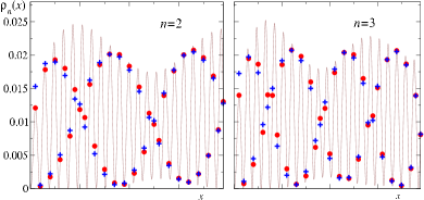
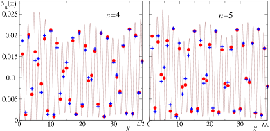
Figure 3: (Color online) DMRG data for the total LDOS of different levels $n$ for $U=1.4t$ (blue crosses) compared to the bosonization results in Eq. (7) with $a=0.56$ (solid line). Red dots mark the LDOS from bosonization at discrete lattice points.

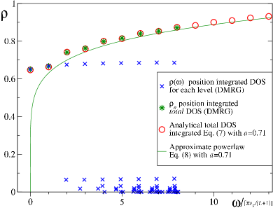
Figure 4: (Color online) DMRG data for $U=1.8t$ and $L=78$ of the position integrated DOS $\rho(\omega)=\sum_{x}\rho(\omega,x)$ for each individual state (blue crosses). The green stars represent the sum over all nearly degenerate states at each discrete energy $\omega_{n}$, which agrees very well with the integral of Eq. (7) (circles).

The number of nearly degenerate states at each energy $\omega_{n}$ grows rapidly with the number of partitions $\sim\exp(\pi\sqrt{2n/3})/4n\sqrt{3}$ and each of those states has an increasingly complex wavefunction, so that a description in terms of approximate powerlaws is normally used. Indeed, if the position dependence is integrated over, the total DOS $\rho_{n}=\sum_{x}\rho_{n}(x)$ in Eq. (7) should follow an approximate powerlaw

$$\rho_{n}\approx\tfrac{1}{\Gamma(1+2\beta^{2})}\left(\tfrac{\pi a}{L+1}n\right)^{2\beta^{2}}=\tfrac{1}{\Gamma(1+2\beta^{2})}\left(\tfrac{a}{v_{F}}\omega_{n}\right)^{2\beta^{2}}.$$ (8)

However, this only holds for the sum over all nearly degenerate states. The individual states on the other hand show a much more interesting energy dependence of the position integrated DOS as shown in Fig. 4. The dominant spectral weight in each multiplet has evolved from the original simple excitation in Eq. (3) (type $|a\rangle$), which has a surprisingly flat energy dependence. The many-fermion states (type $|b\rangle$) are much more numerous, but have a much smaller DOS.

The position integrated total DOS of each level in Fig. 4 agrees well with the integral of Eq. (7). There is no sign of any deviations from the low energy theory, which should break down as the cutoff is approached $\omega\sim v_{F}/a$, i.e. before the DOS reaches the non-interacting value of unity. The alternation of the analytical results relative to the powerlaw is due to boundary effects, which induce additional oscillations with $\sin 2\omega x/v_{F}$ Eggert2000 . In general, for longer range interactions it is also possible to use a momentum dependent Luttinger liquid parameter longrange .

The situation as shown in Fig. 4 is actually quite generic for interacting systems also in higher dimensions: The single particle spectral weight is spread over many-body excitations, thereby renormalizing position, width, and total weight. Our results show quantitatively how an effective finite lifetime of quasiparticle states evolves due to a spread over many-body states.

In one-dimensional systems with spin degrees of freedom $\sigma=\uparrow,\downarrow$, the excitations can be described by two independent bosonic theories for spin and charge egg07 . The spectrum is again given in the form of nearly degenerate multiplets $\omega=\omega_{n_{s}}+\omega_{n_{c}}$, but now labeled by two quantum numbers $(n_{s},\ n_{c})$ for spin and charge with $\omega_{n_{s}}=v_{s}k_{n_{s}}$ and $\omega_{n_{c}}=v_{c}k_{n_{c}}$, where $v_{c}=v_{s}$ in the non-interacting case. A single particle state $c_{n,\sigma}^{\dagger}|N_{0}\rangle$ is now divided over all spin and charge multiplets $(n_{s},\ n_{c})$ corresponding to the different possibilities to write the sum $n={n_{s}}+{n_{c}}$. However, for a given $n={n_{s}}+{n_{c}}$ the multiplets $(n_{s},\ n_{c})$ may now be of quite different energy, since in general $v_{c}>v_{s}$ for repulsive interactions. The spectral weight is therefore spread into several non-degenerate spin and charge multiplets, which is fundamentally different from higher dimensional systems. Moreover, the degeneracy within each multiplet is also lifted in the same fashion as above. In each multiplet there is again exactly one dominant state. The LDOS also shows a very interesting superposition of spin and charge density waves Anfuso2003 , which can be calculated in detail with rescaled waves $\chi_{\ell}(x)/\sqrt{2}$ in Eq. (7). However, the smoking gun for Luttinger liquid behavior in a finite wire would be to identify the increasing number of states due to spin-charge separation and the degeneracy splitting with increasing $\omega$, which is very different from an equally spaced single particle spectrum. Numerically, however, the important effects of interactions can be much better illustrated using the single channel (spinless) case discussed here, which avoids the complications of a huge number of states and a superposition of spin and charge standing waves.

In summary, we were able to describe the LDOS for finite quantum wires in detail by a combination of analytical and numerical methods. The analytical results allow the calculation of the total LDOS in each multiplet. The DMRG calculations give the detailed distribution of local spectral weights over all many-body states in the low energy region. The combination of both methods shows explicitly how the wavefunctions and boson representations of excited states evolve as interactions are turned on. The cutoff parameter $a(U)$ and the normalization in Eq. (6) can be determined from DMRG for the standard model in Eq. (2). Our results show that powerlaws are not sufficient to adequately describe the low energy behavior of individual levels. Instead, a large number of discrete states with varying spectral weights and oscillating wavefunctions would be the generic signature of Luttinger liquid behavior in finite wires. The number of many-body states with non-zero spectral weight is small for the first few levels, but increases exponentially with energy.

Acknowledgments We are grateful to M. Andres, S. Reyes and S. Söffing for helpful discussions and the SFB/Transregio 49 for financial support. I. S. acknowledges support of the Graduate Class of Excellence MATCOR funded by the State of Rheinland-Pfalz, Germany.

References

- (1) M. Bockrath, D.H. Cobden, J. Lu, A.G. Rinzler, R.E. Smalley, L. Balents, and P.L. McEuen, Nature 397, 598 (1999).
- (2) Z. Yao, H.W. Ch. Postma, L. Balents, and C. Dekker, Nature 402, 273 (1999).
- (3) O.M. Auslaender, H. Steinberg, A. Yacoby, Y. Tserkovnyak, B.I. Halperin, K.W. Baldwin, L.N. Pfeiffer, and K.W. West, Science 308, 88, (2005).
- (4) O.M. Auslaender, A. Yacoby, R. de Picciotto, K.W. Baldwin, L.N. Pfeiffer, and K.W. West, Science 295, 825, (2002).
- (5) H. Steinberg, O.M. Auslaender, A. Yacoby, J. Qian, G.A. Fiete, Y. Tserkovnyak, B.I. Halperin, K.W. Baldwin, L.N. Pfeiffer, and K.W. West, Phys. Rev. B 73, 113307 (2006).
- (6) J. Lee, S. Eggert, H. Kim, S.-J. Kahng, H. Shinorara, Y. Kuk, Phys. Rev. Lett. 93, 166403 (2004).
- (7) L.C. Venema, J.W.G. Wildöer, J.W. Janssen, S.J. Tans, H.L.J.T. Tuinstra, L.P. Kouwenhoven, and C. Dekker, Science 283, 52 (1999).
- (8) S.G. Lemay, J.W. Janssen, M. van den Hout, M. Mooij, M.J. Bronikowski, P.A. Willis, R.E. Smalley, L.P. Kouwenhoven, C. Dekker, Nature 412, 617 (2001).
- (9) S. Eggert and I. Affleck, Phys. Rev. B 46, 10866 (1992); Phys. Rev. Lett. 75, 934 (1995).
- (10) M. Fabrizio and A.O. Gogolin, Phys. Rev. B 51, 17827 (1995).
- (11) S. Eggert, H. Johannesson, and A. Mattsson, Phys. Rev. Lett. 76,1505 (1996).
- (12) A.E. Mattsson, S. Eggert, and H. Johannesson, Phys. Rev. B 56, 15615 (1997).
- (13) V. Meden, W. Metzner, U. Schollwöck, O. Schneider, T. Stauber, and K. Schönhammer, Eur. Phys. B 16, 631 (2000).
- (14) S. Eggert, Phys. Rev. Lett. 84, 4413 (2000)
- (15) P. Kakashvili, H. Johannesson, and S. Eggert, Phys. Rev. B 74, 085114 (2006).
- (16) F. Anfuso and S. Eggert, Phys. Rev. B 68, 241301(R) (2003)
- (17) H. Benthien, F. Gebhard, and E. Jeckelmann, Phys. Rev. Lett. 92, 256401 (2004).
- (18) S.R. White, Phys. Rev. Lett. 69, 2863 (1992); Phys. Rev. B 48, 10345 (1993).
- (19) For a review see S. Eggert, Theoretical Survey of One Dimensional Wire Systems, edited by Y. Kuk, et al. (Sowha Publishing, Seoul, 2007), p. 13; arXiv:0708.0003.
- (20) K. Schönhammer and V. Meden, Phys. Rev. B 47, 16205 (1993).
- (21) I. Schneider and S. Eggert, unpublished.